The Outburst of HST-1 in the M87 Jet

Abstract

The X-ray intensity of knot HST-1, 0.85^′′ from the nucleus of the radio galaxy M87, has increased by more than a factor of 50 during the last 5 years. The optical increase is similar and our more limited radio data indicate a commensurate activity. We give the primary results of our Chandra X-ray Observatory monitoring program and consider some of the implications of this extreme variability in a relativistic jet. We find that the data support a ’modest beaming synchrotron’ model as indicated in our earlier papers. Based on this model, the decay of the X-ray lightcurve appears to be dominated by light travel time across the emitting region of HST-1, rather than synchrotron loss timescales.

1. Introduction

This paper is the third from a project to monitor the M87 jet with the Chandra X-ray Observatory with complimentary data from the Hubble Space Telescope (HST), and more recently with the Very Large Array (VLA) and the Very Long Baseline Array (VLBA). The main goal of the project was based on the premise that synchrotron X-ray emission would come from electrons with halflives of order a year or less whereas inverse Compton X-ray emission would come from very low energy electrons with halflives exceeding $10^{4}$ years (Harris & Krawczynski, 2002). In Harris et al. (2003) (hereinafter ’Paper I’) we reported the results from the first year, 2002Jan-Jul. The main findings were significant intensity variability of the core (expected), and of HST-1, a knot in the jet 0.85^′′ (65pc projected) from the core. We argued that the intensity changes were larger for the harder X-ray bands and suggested a synchrotron loss model with modest beaming (Doppler factor, $\delta$, of order 3 or 4, in agreement with earlier proper motion studies; Biretta, Sparks, & Macchetto (1999)). In Perlman et al. (2003) (Paper II), it was suggested that the timescale for optical decay of the lightcurve for HST-1 was similar to the X-ray decay time, and thus not the factor of 10 longer which was predicted by our original synchrotron loss model. Since the measured decay time was based on only a single minor change of optical intensity for each color, we consider this question still open.

In this paper we concentrate on the recent Chandra data from 2003-2005 but will also include optical and radio data for HST-1 as required, leaving the details to other papers in preparation. The ’giant flare’ of HST-1 (the X-ray intensity increased by a factor of 50 in 4 years) has forced us to abandon our original methods of data reduction which were devised the first year of our monitoring when ACIS pileup was not a problem. [‘ACIS’ is the acronym for the Advanced CCD Imaging Spectrometer and ‘pileup’ is discussed in section 3.2.] After a short section on the observations (§ 2) we deal with the data reduction methods and give the basic results for each type of measurement (§ 3). We review the synchrotron parameters in § 4, and discuss implications of the lightcurve timescales in § 5.

We take the distance to M87 to be 16 Mpc (Tonry, 1991) so that one arcsec = 77pc. We use the conventional definition of spectral index, $\alpha$: flux density, S${}_{\nu}~{}\propto~{}\nu^{-\alpha}$.

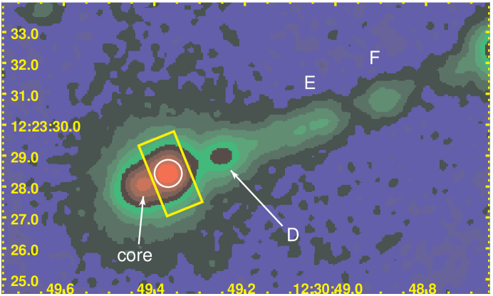
Figure 1.— The inner section of the M87 X-ray Jet: a stacked image from epochs A to V with an effective exposure time of order 110ks. The data come from evt2 files so the true (average) intensity of HST-1 is underestimated because of pileup. The coordinates labels are Right Ascension and Declination in J2000. The intensity units are electron volts per second per 0.0492 arcsec pixel, and the peak value is 5.5. The faintest red corresponds to 0.5 and the black below the green is close to 0.01. The yellow rectangle around HST-1 is that used for the lightcurve photometry and the small circle is that used in PapI (sections 3.2, 3.3.).

2. Observations

The first Chandra observations of M87 that specifically targeted the jet were those done by Wilson in 2000 Jul (Wilson & Yang, 2002; Perlman & Wilson, 2005). They experimented with various ACIS frame times in order to minimize the effects of pileup (two or more photons arriving at the same pixel during the same frame time, thus masquerading as a single event with the sum of the energies; see, e.g. Davis (2001)). They found that a frame time of 0.4s gave essentially the same countrate as 0.1s for the nucleus of M87 which, at that time, was the brightest feature. Thus we adopted the same ACIS setup: chip S3 (back illuminated for low energy response), 1/8th subarray, and 0.4s frame time. A list of our observations is given in Table 1. Basically, we have been getting a 5 ks observation approximately every 6 weeks for four ’seasons’: mid November to early August (when M87 is far enough from the Sun to be observable with Chandra and the HST). Our approved proposal for Chandra AO7 will continue this strategy (2005Nov to 2006Aug). During the 2005 season we have obtained an extra 5 observations designed to give us weekly coverage for 2 months to check for shorter timescale changes.

Table 1Chandra dates and X-ray intensities of HST-1

Observational Parameters				Intensities of HST-1
Epoch	Date	Obsid	Livetime	Ka	f(0.2-6keV)b	S(2keV)c
label			(sec)	(keV/s)	(10-12 cgs)	(nJy)
Ad	2000Jul30	1808	12845	0.247	0.729	29.2
B	2002Jan16	3085	4889	0.734	2.32	92.8
C	2002Feb12	3084	4655	0.588	1.87	74.8
D	2002Mar30	3086	5089	0.576	1.84	73.6
E	2002Jun08	3087	4973	0.798	2.57	102.8
F	2002Jul24	3088	4708	1.096	3.54	141.6
G	2002Nov17	3975	5287	0.799	2.62	104.8
H	2002Dec29	3976	4792	0.653	2.14	85.6
I	2003Feb04	3977	5276	0.645	2.12	84.8
J	2003Mar09	3978	4852	0.872	2.88	115.2
K	2003Apr14	3979	4492	1.071	3.54	141.6
L	2003May18	3980	4788	1.022	3.39	135.6
M	2003Jul03	3981	4677	0.859	2.86	114.4
N	2003Aug08	3982	4841	1.214	4.06	162.4
O	2003Nov11	4917	5028	2.192	7.36	294.4
P	2003Dec29	4918	4677	2.041	6.88	275.2
Q	2004Feb12	4919	4703	4.079	13.81	552.4
Re	2004Mar29	4920	5235	..	..	..
S	2004May13	4921	5251	5.358	18.23	729.2
T	2004Jun23	4922	4543	5.323	18.16	726.4
U	2004Aug05	4923	4633	5.636	19.28	771.2
V	2004Nov26	5737	4237	7.494	25.76	1030
W	2005Jan24	5738	4666	8.316	28.66	1146
X	2005Feb14	5739	5154	8.785	30.30	1212
Ya	2005Apr22	5740	4699	12.42	42.91	1716
Yb	2005Apr28	5744	4699	12.17	42.08	1683
Yc	2005May04	5745	4705	11.80	40.81	1632
Yd	2005May13	5746	5142	11.60	40.14	1606
Ye	2005May22	5747	4701	11.24	38.92	1557
Yf	2005May30	5748	4699	10.66	36.92	1477
Yg	2005Jun03	5741	4698	10.43	36.14	1446
Yh	2005Jun21	5742	4703	10.27	35.58	1423
Yi	2005Aug06	5743	4672	7.105	24.64	985.5

Note. – All observations had 1/8th subarray ACIS-S7 chip only, and 0.4s frame time.
^a The values of K are our primary measured quantity. They come from summing the energies of all events (from the ’evt1’ file) within a rectangle of length 5 pixels transverse to the jet and 2.5 pixels along the jet (fig. 1). The upstream edge is approximately midway between HST-1 and the core component. No background subtraction was employed: when the source is weak, the background (in counts) is of order 1%, and for the highest intensity, the background is less than 0.3%. There is no correction for the buildup of ACIS contamination.
^b f(0.2-6keV) is the observed X-ray flux (the flux density integrated from 0.2 to 6 keV) with units of 10^-12 erg cm^-2 s^-1. An approximate correction has been made for ACIS contamination buildup but not for Galactic absorption.
^c The flux density at 2 keV has been calculated from the observed flux assuming a spectral index, $\alpha$=1.5. For $\alpha$=1.75, the listed values should be reduced by a factor 0.75 and for $\alpha$=1.25, they should be increased by a factor of 1.25. 1 nJy is 10^-32 erg cm^-2 s^-1 Hz^-1.
^d Archival data from Wilson & Yang (2002).
^e This observation was taken in continuous clocking mode, so there is no 2D image available.

3. Data reduction and basic results

While we have maintained a fixed observing strategy, the data reduction has been done over the course of several years and thus the software reduction package, ‘CIAO’ (Chandra Interactive Analysis of Observations), has evolved through several releases, as has the calibration database. However, all data except the ’keV/s’ values have been corrected for the contamination on the ACIS detector, and we are not aware of any software or calibration changes that would adversely affect our results.

The essential preparatory procedures are removal of the pixel randomization and registration to align the X-ray core with the radio core. After setting up the bad pixel file and checking the lightcurve of a large background region for flares (since we use small extraction regions and no large flares were found, we did not time filter any observation), we removed the pixel randomization imposed by the standard pipeline by following the relevant CIAO thread. Registration of the X-ray image was accomplished by measuring the apparent positions of the core and knot A on both radio and X-ray images (the latter binned to 1/10th native ACIS pixel and smoothed with a Gaussian of FWHM=0.25^′′), and then changing the values of the FITS header keywords in the Chandra event file. In general, this procedure introduces an uncertainty of approximately 0.05^′′ or less for the early part of the program when the intensity of the core was comparable to that of HST-1. However, when HST-1 became more than 10 times brighter than the core, our ability to determine the centroid of the core emission is compromised, and we then gave more weight to the position of knot A which is not so well determined because knot A is resolved.

3.1. Intensities from fluxmaps

The original data reduction procedure is outlined in Paper I and involves constructing monochromatic exposure maps for three energy bands. Dividing the data by the exposure map we obtain 3 flux maps. Each flux map was then multiplied by $h\nu_{\rm nom}$ to obtain units of ergs cm^-2 s^-1. $\nu_{\rm nom}$ corresponds to the nominal energy for each band (chosen to approximate the band center weighted by the effective area) which was used to construct the relevant exposure map. This permits us to measure fluxes with normal photometric procedures. All that is required is to sum the flux within a measuring aperture and multiply the result by the ratio of the mean energy of events within the aperture to the nominal energy of the band being measured. We have redone the fluxmaps now that CIAO automatically corrects the exposure maps for ACIS contamination buildup. Previously we had used a fixed region of M87’s thermal hot gas emission to make this correction.

When using small apertures (our standard region was a circle with r=0.44^′′ in order to separate the core from HST-1; see fig. 1) a point spread function (PSF) correction of 1.55$\pm$0.05 is required to ’recover’ the fraction of the PSF outside the small circle. Although it is known that the PSF size is a function of energy, from our PSF simulation with ChaRT/Marx, we found values between 1.50 and 1.60 for our 3 energy bands. From the same simulations, we find that 6$\pm$4% of each PSF falls within the adjacent measuring aperture (this is for the special case of the small circles for the core and HST-1). In Paper I, these corrections had not yet been devised, so the flux scales in the figures should not be used to derive absolute values. We provide our best flux estimates later in this paper.

3.2. Intensities from piled up data: keV/s

Pileup for CCD’s occurs when two or more events are received for the same pixel during a single frame time (Davis, 2001). Thus we lose the inherent spectral energy distribution one normally associates with ACIS data. However, to first order, the energy content of the arriving photons is preserved and a measure of the total band is still available. To obtain intensities for lightcurves, we first followed the ’afterglow thread’ to recover the events with grade migration that caused them to be mistaken for afterglow events. Then we checked to see that all events of interest would be accepted by a suitable energy filter. The incident spectrum of HST-1, both as measured when the knot was weak (essentially no pileup) and from our observation in continuous clocking mode, is essentially contained in the band 0.2 to 6 keV (probably 95% of the counts are below 4 keV). To recover the energy associated with piled events that now appear above 6 keV, we examined the event file at the higher energies and set the upper cutoff to a value that includes all events associated with HST-1 (up to 17 keV in some cases).

The CIAO tool ’dmstat’ then gives the total energy (in eV) of all events. Dividing this by 1000$\times$livetime (where ‘livetime’ is the total time the detector is accumulating data) provides an intensity measurement in keV/s. Through early 2004, pileup was fairly mild, so we continued measuring the event2 file. As the pileup increased, we found we were losing more and more events to grade migration so the data shown in fig. 2 are based on the event 1 file with no grade filtering and only the standard good time intervals applied. A rectangular extraction region (see fig. 1) was used for this photometry.

Figure 2.— Multi-wavelength lightcurves for knot HST-1 in the M87 jet. The left panel shows the X-ray, and UV lightcurves on a linear scale to more clearly show the higher levels. On the right is the same plot on a log scale in order to better compare slopes (percentage changes). For this version we have added radio data at 15 GHz (the 2000 datum comes from an archival VLA observation). Both X-ray curves are from the evt1 files in keV/s. For the UV data, the left panel has units of 0.1 mJy whereas on the right, the units are mJy.

There are several limitations to this method. It is impossible to get spectral information like band fluxes; there is no a priori method to correct for ACIS contamination buildup; and there may have been bona fide events that were rejected by on-line software aboard the satellite and thus are unrecoverable. In spite of these deficiencies, this ’keV/s’ method provides a reasonably direct estimate of the total observed intensity.

3.3. Problems Associated with the Spectral Analyses

For spectral analyses of HST-1 there are between several hundred and more than 3000 counts in a typical 5ks observation. We have performed spectral fits for simple power laws (PL), power laws with a high energy cutoff (cutPL), and both models in conjunction with the ’jdpileup model’ (Davis, 2001), as implemented in Sherpa (Freeman et al., 2001). There are a number of problems.

The jdpileup model, even with the ’Monte-Powell’ method which is advertised as being the best option to locate the true minimum in chi-squared, can produce a best fit which is obviously wrong: the fit gives an amplitude which is up to a factor of 10 too large, with an excessively large pileup fraction. This formal fit occurs because the fit finds a solution on the heavily piled up section of the pileup curve (Davis, 2001, fig. 6). This is particularly evident for featureless spectra such as power laws. In the fitting algorithm, there is a ’degeneracy’ for featureless spectra between the power law exponent and the pileup ’survival probability’ parameter, jdp.alpha.

The only way we found to mitigate this problem was to constrain several fit parameters: Nh, the total column density of neutral hydrogen per square cm towards the source, was forced to be at least the Galactic value of 2.5$\times 10^{20}$ cm^-2 (Stark et al., 1992); the survival probability parameter jdp.alpha.min=0.2; and the spectral index, $\alpha$, was constrained to lie between 0 and 3. It was also necessary to pick good values for the initial guess for jdp.alpha, $\alpha$, and the amplitude of the power law.

Another uncertainty is the mutual dependence between Nh and $\alpha$ which can be demonstrated by a simple example using the spectral file for HST-1 from epoch D. The power law fit gives Nh=(3.4, +1.9, -1.5)$\times 10^{20}$cm^-2 and $\alpha$=1.46$\pm$0.14. Freezing Nh to values of 2.5, 3.5, and 4.5$\times$10²⁰, results in $\alpha$ values of 1.39$\pm$0.07, 1.47$\pm$0.07, and 1.54$\pm$0.08 respectively. Although it is conceivable that Nh could vary because HST-1 is at a projected distance of only 65pc from the nucleus of M87 and its diameter is less than a parsec, we assume it is constant, possibly augmented by an excess absorption above the Galactic value, i.e. intrinsic to M87. From spectral fits before pileup became a problem, we find fit values of Nh which average 3.5$\times 10^{20}$cm^-2 (i.e. a bit larger than the Galactic value), although each individual solution is consistent, within the errors, with the Galactic value.

A further effect complicates the solution. The pileup effect we call ’Eat Thy Neighbour’ comes into play for two close sources. If a core photon arrives during the same frame time as a photon from HST-1, often they will be within each other’s 3x3 pixel region and thus be interpreted as a single event at the location of the pixel with the larger energy.

Finally, the value of $\alpha$ depends on the choice between a simple power law and a power law with an exponential cutoff. Although in many cases the value of the cutoff energy is very large and the $\alpha$’s of PL and cutPL are sensibly the same, for other cases for which the fit value of the cutoff energy is below 12 keV, the corresponding values of $\alpha$ for the two models diverge with a concomitant shift in the fit value of Nh (an example is given in Table 2).

Table 2Spectral Parameters for the CC mode data on HST-1

Model	Nh	$\alpha$	$\chi^{2}$
	1020cm-2
power law (PL)	7.3$\pm$0.9	1.72$\pm$0.06	0.42
PL (BGsubtract)	6.6$\pm$0.9	1.73$\pm$0.06	0.40
PL + cutoff	2.5$\pm$0.4	1.18$\pm$0.11	0.51

Note. – For the PL + cutoff, the high energy cut value is 3.7$\pm$1.1 keV and the value of Nh is the lowest allowed (set to the Galactic value).

Considering these difficulties, we believe it would be premature to present a table of spectral parameters. For the 2002 to 2003 data (prior to the large intensity increase), with Sherpa we find $\alpha\approx$1.5$\pm$0.3, and Nh appears to be consistent with, or a bit larger than, the Galactic value. A joint fit of these data with XSPEC constraining Nh to a common value but allowing amplitude and spectral index to vary for each observation, results in Nh=(2.6$\pm$0.5)$\times$10²⁰ cm^-2 and $\alpha$ ranging from a minimum of 1.1 to a maximum of 1.5. It is our opinion that with spectral fitting, we cannot confidently claim that the spectrum of HST-1 is harder or softer when the intensity is high.

Given the sizable uncertainty in spectral parameters of HST-1 from piled up data, we proposed a 10ks observation for Director’s Discretionary Time to obtain a continuous clocking (CC) mode observation to be made during those few days in 2004March when the CCD readout direction is orthogonal to the jet. The idea was that we could obtain one set of reliable spectral parameters and compare them to those obtained from our normal 5 ks observation which was already scheduled for the last week of March. Our proposal was not granted time, but we were allowed to change the mode of our normal 5 ks observation to CC mode.

In CC mode pileup is not a problem since the readout is continuous and each pixel is effectively moved every 41 $\mu$s. We followed the thread to correct the time of each event from the readout time to the arrival time, thus ensuring that the correct aspect solution would be applied. A profile along an East-West line (i.e. the jet is projected onto the RA axis from its normal position angle 20^∘ away) is shown in fig. 3.3. We then isolated knot A, HST-1, and the core with thin rectangles on the 1D ’image’ of the event file. Notwithstanding the fact that there are no accurate calibration files for CC mode, we generated ’pha files’ (the collected events with their energies) and corresponding effective area and redistribution matrices to permit us to run normal Sherpa spectral analysis. Background areas on each end of the jet were used. The spectral results are given in Table 2.

The profile of the jet along the RA axis of the observation of 2004Mar29 (Epoch R) taken in the continuous clocking mode. The resolution is 0.1 native ACIS pixels, or 0.0492^′′. Emission from the core, with an intensity similar to knot A (the feature towards the right), is lost on the left flank of HST-1, the dominant feature. The location of the core should be 1.6 pixels to the left of HST-1. Note the relatively poor s/n of knot A, since the profile contains the background from the whole chip.

The CC mode observation was meant to confirm the jdp spectral parameters, but insofar as $\alpha$ is concerned, the CC fit gives a significantly larger value than the preceeding and following values. At this time, we do not know how to decide if the CC value is wrong because of unreliable calibration files, or if the jdp values are (systematically) too small. We note that whereas for the normal 2D image analysis, the background level has essentially no effect on the spectral fit since the measuring aperture is so small, this is not the case for the CC mode, for which the background of each pixel comes from an entire column in chip coordinates. While we cannot be certain that the spectrum of HST-1 did not change markedly during the months surrounding the CC observation, this seems unlikely. Although the CC experiment failed to provide higher accuracy for the spectral parameters, the range of values in Table 2 is still within the ranges for HST-1 prior to the major intensity increase.

3.4. Fluxes and flux densities

While most fluxes quoted from Chandra data are based on the usual spectral analyses (sec. 3.3), we favor fluxes from fluxmaps as being a quantity which is closer to an ’observable’ and less susceptable to model assumptions. As described above, measuring on flux maps achieves this objective when pileup is not a problem. To generate approximate fluxes from the observed keV/s measurements, we convert keV to ergs and divide by the effective area.

Since all indications are that most of the flux falls within the 0.2 to 6 keV band, we take a nominal effective area of 400 cm² as a first guess for the spectrum of HST-1 weighting the Chandra effective area. We then calculate a flux:

$F(0.2-6~{}keV)=1.602\times 10^{-9}\frac{K}{400~{}\times~{}a}=4.00\times 10^{-12}~{}\frac{K}{a}$ erg cm${}^{-2}~{}$s^-1

where K is the measured keV/s value and $a$ is a correction factor for the (unknown) effective area which is a function of time because of the ACIS contamination buildup.

We find the values of $a$ by comparing F(a=1) with the flux measured on the flux maps for those observations made in 2002 and 2003 before pileup became a serious problem. We find a(2000.5828)=1.356, thereafter declining to values around 1.2 by mid 2003. Making a rough extrapolation of a(t) permits us to make a first order correction for the contamination problem. We estimate that resultant uncertainties are of order 15%, based on the scatter of a(t) from a smooth curve. Fluxes are listed in Table 1. In the same table we give flux densities at 2 keV calculated from the flux values assuming $\alpha$=1.5.

4. Synchrotron Parameters

In this section we examine the physical parameters associated with the synchrotron emission model in the same context as used in Paper I: we use the rise time to estimate the physical diameter and the decay time to constrain the beaming factor, assuming E² losses dominate.

For a given interval, $\Delta$t, we measure a fractional increase of y=I₂/I₁. Then the doubling time, dt= [(1/(y -1)]$\times\Delta$t, and the doubling time in the jet frame is dt^′ = $\delta\times$dt yr. Thus the diameter of the emitting region will be d $\leq$ dt^′/3.26 pc and the radius, r = d/(2$\times$77) arcsec. From inspection of fig. 2, we select a number of intervals with large rate of increase and in Table 3 we give the calculated doubling times. For a selection of values for the beaming factor, in Table 4 we give the corresponding upper limit to the sizes of the emitting region for a characteristic doubling time of 0.14 yr.

Table 3Doubling Times for HST-1

Epoch Interval	$\Delta$t	(y-1)a	dtb
			(yrs)
E-F	0.125	0.373	0.34
I-J	0.090	0.352	0.26
M-N	0.099	0.413	0.24
P-Q	0.123	0.998	0.12
X-Ya	0.183	0.413	0.44

Note. – With a statistical error of a few percent on each intensity measurement, we estimate the uncertainties of the doubling times are dominated by systematic errors of order 15%.
^a y is the intensity ratio, I₂/I₁.
^b dt is the doubling time in our frame.

Table 4Size of Emitting Region for HST-1

$\delta$a=	1	3	5	9	12	20	40
dt′(yrs) =	0.14	0.42	0.70	1.3	1.7	2.8	5.6
diameter(pc) =	0.043	0.13	0.22	0.39	0.52	0.86	1.72
radius(arcsec) =	0.00028	0.00084	0.0014	0.0025	0.0034	0.0056	0.011

Note. – For an observed doubling time of $\approx$0.14 years, we calculate maximum values for the source size.

We construct a spectrum for 2005Jan1 with data from the VLA; at 220nm from the Hubble Space Telescope; and our Chandra value for Jan 2005 from Table 1. This is shown in fig. 4. We then convert the frequencies and flux densities to the jet frame and solve for the usual synchrotron parameters (Pacholczyk, 1970): see Table 5.

The spectrum of HST-1 around 1 Jan 2005. The radio flux densities are from the VLA; the UV from the HST; and the Chandra interpolated from Table 1. The two point spectral indices are $\alpha_{\rm r-UV}$=0.45 (22GHz to 220nm) and $\alpha_{\rm ox}$=1.03 (220nm to 2 keV).

Table 5Synchrotron Parameters for HST-1

$\delta$	radius	Beq	R	log Etot	P	$\tau^{\prime}_{\rm UV}$	$\tau_{x}^{\prime}$/d(l.y.)	$\tau_{x}$
	(cm)	(gauss)		(ergs)	(erg s-1)	(yrs)	(ly)	(yrs)
1	8.3$\times 10^{16}$	0.10	1.67	48.72	1.2$\times 10^{42}$	0.015	0.02	0.0015
3	2.5$\times 10^{17}$	0.01	0.084	48.11	1.0$\times 10^{41}$	0.91	0.32	0.030
5	4.1$\times 10^{17}$	0.0037	0.021	47.82	3.1$\times 10^{40}$	6.03	1.34	0.10
9	7.5$\times 10^{17}$	0.0010	0.0043	47.50	8.4$\times 10^{39}$	53.8	6.48	0.60
20	1.6$\times 10^{18}$	0.0002	0.0006	47.05	1.3$\times 10^{39}$	894	50.2	4.47

Note. – The HST-1 spectrum used is that of fig. 4.

We have identified the most rapid decay rates, and these are given in Table 6. Estimates of the time for the intensity to drop by a factor of two range from 0.2 to 0.3 years. Matching 0.2 yrs to the results of Table 5, we find $\delta$=6.3, a value somewhat higher than that found in Paper I and also larger than the models reported in Table 3 of Biretta, Sparks, & Macchetto (1999) for the 6c proper motions in HST-1. However, the X-ray decay time is remarkably close to the rise time (which we used to estimate the source size), so it seems likely that both rise and fall reflect the time required to cross the source, and not the E² half-life. Although this is not proven, for the remainder of this paper we adopt the view that the X-ray decay time reflects the light travel time across HST-1. Thus solutions for smaller $\delta$ (e.g. 3 to 5) are favored. Given the assumptions of the model, $\tau_{x}^{\prime}$=diameter(l.y.) for $\delta\approx 4.6$ (see the next to last column in Table 5). For smaller $\delta$ the lightcurve decay should be dominated by light travel time; for larger $\delta$ the weaker magnetic field leads to longer E² halflives. Large $\delta$ (e.g. 20) values are disfavored because of their large $\tau$ values and the much smaller angles to the line of sight which would be required.

In Paper I we argued that the total emission of HST-1 did not impose any significant drain on the total estimated energy flow down the jet. This continues to be the case so long as $\delta$ is $\geq$ 3. The power needed to generate the required total energy in the time dt^′ (the jet frame doubling time) is listed in Table 5. These values may be compared to the estimate of Young et al. (2002) for the jet’s kinetic energy flow of 3$\times~{}10^{42}$ erg s^-1, based on energetics of the interaction between the jet and the ISM which are not based on particular jet models. The power required to explain the observed flare in M87 would be comparable to the jet’s kinetic energy only if there were no beaming, an untenable hypothesis.

Table 6Decay times for HST-1

Epoch Interval	$\Delta$t	y	halftime
	(years)		(years)
B-C	0.075	0.801	0.19
G-H	0.111	0.817	0.30
L-M	0.126	0.840	0.40
Ya-Yg	0.115	0.840	0.36
Yh-Yi	0.126	0.692	0.21

Note. – All values are in the observer’s frame.

5. Implications from rise and fall timescales

There is a long history supporting the notion that brightness enhancements occur at the locations of internal shocks which produce power law spectra of relativistic electrons via Fermi acceleration (e.g., Blandford & Königl, 1979). Polarization data support this notion with increased polarizations and electric vectors perpendicular to the knot leading edge. These are characteristic of shocks and are associated with the flux maximum regions (Perlman et al., 1999, 2003).

If we view the shock model as a method of generating a new or augmented power law of relativistic electrons (and increasing the field strength), we note that there is no difficulty with the energetics (see above) and also note that the general behaviour of the lightcurves in fig. 2 demonstrate comparable rates of intensity increase for radio, optical, and X-rays. This is a pre-requisite for the shock model which relies on the power law extending from low values of $\gamma$ up to $\approx~{}10^{7}$. Whether the flare owes its genesis to an increase in delivered energy from the nucleus, or to a change in the size and strength of the shock, is not determined.

The clear prediction resulting from a new power law distribution is that the UV emission should decay 10 times more slowly than the X-rays, and the radio emission should persist much longer because of the $\gamma^{-1}$ dependence of the electron half-life suffering E² losses. This should be observed in the lightcurves so long as the light travel time across the source is significantly less than the half-life. For the synchrotron model described in Table 5, the estimated size (in l.y.) of the emitting region is comparable to the halflife of electrons responsible for the X-ray emission, but less than the predicted half-life for UV emitting electrons. In Paper II, we suggested that the optical decay times were similar to those in the X-rays, but this was based on a quite small intensity drop. Given the marked X-ray decline starting in 2005Apr, this issue should be clarified by optical and radio data obtained in 2005 but not yet available to us.

6. Conclusions

The three lightcurves (X-rays, UV and radio; fig. 2) are parallel to a good accuracy. This means that the input spectrum of relativistic particles which caused the flare did not change its shape, only its amplitude. The “choppiness” in the X-ray light curve may be caused by synchrotron losses which would be much weaker at lower energies.

If we match the observed decay time to the halflife of electrons producing the X-rays, we find $\delta$ a bit larger than 5. However, if the decay time is governed by the source size, as suggested by the near equivalence of rise and decay times, we should choose a $\delta$ which satisfies the condition $\tau_{x}^{\prime}~{}\leq$ diameter(l.y.). This requires $\delta~{}\leq$ 5, and that would be consistent with our results of Paper I that $\delta~{}\approx$ 4.

Radio and optical data now being obtained should provide the basis for ’solving’ two distinct issues: separating light travel time from electron halflives and distinguishing between compression/expansion versus the injection of new particles.

If the decay segments of the lightcurves show longer decay times for lower frequencies, it will be possible to separate the light travel time across the source from E² loss times. From the models already considered, probably the optical, but certainly the radio, halflives should be considerably longer than the light travel time, so the corresponding decay times in these lightcurves will provide a reasonably direct estimate of the halflife against E² losses. Since the magnetic field energy density is greater than the photon energy density in all models considered, we will thus obtain another estimate of the magnetic field strength from the observed halflife.

If however, all bands rise and fall together, the compression/expansion explanation will be supported. Given an emitting region, be it the result of a shock or some other process, a rather modest compression can increase the intensity by the required factor of 50 since all electrons will receive the same percentage energy boost and the field strength will increase. Thus the flare would result from a simple compression without the introduction of ’new particles’. If the subsequent decay of intensity were to arise from an expansion, all bands should drop equally with no delays between bands. Moreover, the relative rate of expansion will be reflected in the light curve. If the decay timescale is comparable to the rise time, this would indicate a rapid expansion (i.e. rapid drop in volume emissivity) whereas a decay significantly slower than the rise would point to a slower expansion. In the latter case, expansion velocities can be estimated from the lightcurve with simple assumptions.

References

- Biretta, Sparks, & Macchetto (1999) Biretta, J. A., Sparks, W. B., & Macchetto, F. 1999, ApJ, 520, 621
- Blandford & Königl (1979) Blandford, R. D., & Königl, A. 1979, ApJ, 232, 34
- Davis (2001) Davis, J. E. 2001, ApJ, 562, 575
- Freeman et al. (2001) Freeman, P., Doe, S., & Siemiginowska, A. 2001, Proc. SPIE, 4477, 76
- Harris & Krawczynski (2002) Harris, D. E. & Krawczynski, H. 2002, ApJ, 565, 244
- Harris et al. (2003) Harris, D. E., Biretta, J. A., Junor, W., Perlman, E. S., Sparks, W. B., & Wilson, A. S. 2003, ApJ, 586, L41
- Pacholczyk (1970) Pacholczyk, A. 1970, Radio Astrophysics (San Francisco: W. H. Freeman & Co.)
- Perlman et al. (1999) Perlman, E. S., Biretta, J. A., Zhou, F., Sparks, W. B., & Macchetto, F. D. 1999, AJ, 117, 2185
- Perlman et al. (2003) Perlman, E. S., Harris, D. E., Biretta, J. A., Sparks, W. B., & Macchetto, F. D. 2003, ApJ, 599, L65
- Perlman & Wilson (2005) Perlman, E. S., & Wilson, A. S. 2005, ApJ, 627, 140
- Stark et al. (1992) Stark, A. A., Gammie, C. F., Wilson, R. W., Bally, J., Linke, R. A., Heiles, C., & Hurwitz, M. 1992, ApJS, 79, 77
- Tonry (1991) Tonry, J. L. 1991, ApJ, 373, L1
- Wilson & Yang (2002) Wilson, A. S. & Yang, Y. 2002, ApJ, 568, 133; Appendum 2004, ApJ, 610, 624
- Young et al. (2002) Young, A. J., Wilson, A. S., & Mundell, C. G. 2002, ApJ, 579, 560