MULTIVARIATE ANALYSIS OF GLOBULAR CLUSTER’S HORIZONTAL BRANCH MORPHOLOGY: searching for the second parameter.

Abstract

Aims. The interpretation of globular cluster horizontal branch (HB) morphology is a classical problem that can significantly blur our understanding of stellar populations.

Methods. In this paper, we present a new multivariate analysis connecting the effective temperature extent of the HB with other cluster parameters. The work is based on Hubble Space Telescope photometry of 54 Galactic globular clusters.

Results. The present study reveals an important role of the total mass of the globular cluster on its HB morphology. More massive clusters tend to have HBs more extended to higher temperatures. For a set of three input variables including the temperature extension of the HB, $[Fe/H]$ and M_V, the first two eigenvectors account for the 90% of the total sample variance.

Conclusions. Possible effects of cluster self-pollution on HB morphology, eventually stronger in more massive clusters, could explain the results here derived.

1 Introduction

Globular clusters (GC), comprised of chemically homogeneous and coeval populations of stars, represent excellent systems for testing stellar models. The various sequences that appear in the colour-magnitude diagram (CMD) of a globular cluster can be compared to the predicted isocrones and theoretical loci. In this way, the properties of stars at different stages of evolution, and the fundamental characteristics of the clusters themselves, such as cluster distance and age, can be derived. Hence, it is not surprising that the study of GCs has played a pivotal role in the development of stellar astrophysics.

In this paper, we will focus on one evolutionary stage: the horizontal branch. HB stars are characterized by core-helium burning and shell-hydrogen burning. The star location in effective temperature along the Zero Age Horizontal Branch (ZAHB) depends on virtually all stellar parameters (composition, age, rotation, etc…, see e.g. Rood 1973). The wide colour distribution of the HB, called the HB morphology, is the result of large differences in the envelope mass of stars having the same core mass, at the same evolutionary stage. The HB phase behaves as an amplifier, displaying the record of both initial conditions and of any variations and perturbations in the evolution of the star from its birth up to the HB stage. Therefore, reading properly the HB morphologies can yield a better understanding of Population II stellar evolution in general, and of the specific stellar systems, clusters or galaxies, in particular.

However, it appears that our comprehension of the HB phase and its precursors is incomplete. Canonical stellar theory can not adequately explain the wide variety of HB morphologies observed in Galactic GCs, ranging from short red HBs to long extended “blue tails”. In particular, blue tails still represent a puzzle in the stellar evolution model, in the sense that we know what the stars in blue tails are, but we do not know how stellar evolution can create them.

To a first approximation, the different temperature extension and morphology of the observed HBs were interpreted in terms of the metal abundance variation, the first parameter: metal-rich clusters tend to have short red HBs, while metal-poor ones exhibit predominantly blue HBs. Nevertheless, the previous approximation turned out to be too rough very soon. Some other parameter (or set of parameters) was evidently also at work, as clusters with nearly identical metallicities could show very different HB colour distributions (van den Berg 1967, and Sandage & Wildey 1967). One classical example is the pair formed by M3 and M13, with $[Fe/H]=-1.57$ and $[Fe/H]=-1.54$ (Harris 1996, in its revised version of 2003) respectively, but very different HB morphologies. The variety of proposed candidates range from cluster age, to helium mixing, [CNO/Fe] abundance, cluster concentration, stellar rotation, planets… In fact, the second parameter problem has already been the object of an extensive list of studies that is important to acknowledge. An increasing amount of observational data progressively revealed the complexity of the scenario (Kraft 1979, Freeman & Norris 1981). Important work was developed by the Yale group (e.g. Lee et al. 1987, 1988, 1990, Sarajedini & King 1989) interpreting cluster age as a global second parameter, in the framework of a Galactic formation picture a la Searle & Zinn (1978). On the other hand, relevant questions outside this scenario were also discussed by different authors (Renzini & Fusi Pecci 1988, Rood & Crocker 1989, Buonanno et al. 1989, Fusi Pecci et al. 1990, Fusi Pecci et al. 1993). In particular, the idea that production of hot HB stars may be somehow influenced by the dynamical processes in the cluster was also carefully explored. In agreement with this, Fusi Pecci et al. (1993) and Buonanno et al. (1997) suggested environement density as a possible second paramenter. Finally, among other more recent works those of Soker & Harpaz (2000) and Catelan et al. (2001) can be cited.

In this work, we have analyzed a homogeneous database of 54 globular cluster CMDs from Hubble Space Telescope photometry in an attempt to quantify the different dependences of HB morphology on cluster parameters: metallicity, concentration, distance to the Galactic center, total mass, etc…, in other words, to search for the so called HB second parameter(s). The data, reduced and treated in an uniform way, represent an exceptional opportunity, from the statistical point of view, to investigate how HB morphology depends on globular cluster properties. On the other hand, the multidimensional data set of Galactic globular clusters spans a large range in many of their properties such as luminosity, metallicity, etc… Therefore, in order to reveal the possible complex correlations hidden in the HB second parameter problem, we decided to apply a multivariate statistical analysis. This approach can not only confirm or reveal new correlations, but offers the possibility to estimate the relative importance of the various HB dependences and the degree of explanation of HB morphology that can be obtained by their combination. A similarly motivated study was already done by Fusi Pecci et al. (1993). We believe that our new, HST-based data set warrants a fresh look at the problem.

2 The database

The analysis presented here is based on a Hubble Space Telescope snapshot program aimed at mapping the cores of all GCs with (m-M)_B $<$ 18.0, using the Wide Field/ Planetary Camera 2 (WFPC2) of HST. All the photometric data come from HST/WFPC2 observations in the $F439W$ and $F555W$ bands, the WFPC2 equivalents of the $B$ and $V$ filters, which are suited for a generic survey and constitute the best choice to identify new anomalous HBs. In all cases, the PC camera was centered on the cluster center.

The colour-magnitude diagrams and the photometry derived from that program have been already published by Piotto et al. (2002). Moreover, the database has already given rise to a number of works attacking still-open topics on evolved stars in GCs (Piotto et al. 1999, Palmieri et al. 2002, Raimondo et al.  2002, Zoccali et al. 1999, Bono et al.  2001, Zoccali et al.  2000, Cassisi et al. 2001, Riello et al. 2003, Recio-Blanco et. al. 2004, Piotto et al. 2004, Salaris et al. 2004, De Angeli et al. 2005 ). The complete database consists in a total of 74 GCs (53 snapshot plus 21 archive data). For this work, only those clusters whose CMD had a well populated HB and enough photometric precision to offer reliable estimations of HB temperatures, 54 of them, were used.

Due to the severe stellar crowding, the excellent resolving power of HST is crucial for the photometrical studies of the globular cluster central regions, where accurate ground based observations are precluded. Moreover, for GCs near the Galactic center, only the central regions are sufficiently uncontaminated by field stars to allow a good study of the colour-magnitude diagram.

3 Considered cluster parameters

3.1 The morphology parameter: maximum effective temperature along the HB

The first step in this work consists in the evaluation of the HB morphology of each cluster. In order to have a quantitative measure of their extension, we determined the highest effective temperature reached by the stars in the HBs of all the clusters in our data set by fitting a Zero Age Horizontal Branch (ZAHB) model to the observed CMDs. In this way, we can study how the extension of the horizontal branch varies with cluster parameters. It is worth to mentioning, however, that HB bimodality, i.e. the presence of both a red HB and a blue tail as in NGC2808, is not been taken into account with this approach.

ZAHB models from Cassisi et al. (1999) were fitted to our $F439W,F555W$ CMDs using the values of distance modulus and reddening derived in our previous paper, Recio-Blanco et al. 2004, for each of the clusters in the data set.

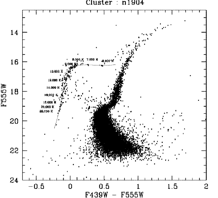
Figure 1: ZAHB model by Cassisi et al. (1999) fitted to NGC 1904 colour-magnitude diagram. The effective temperature variation along the HB is also shown.

This procedure allowed us to evaluate the highest $T_{\rm eff}$ reached by the globular cluster HB and therefore its temperature extension, as illustrated in Figure 1 for the case of NGC 1904 for which the corresponding temperatures along the HB are marked. The errors in this temperature determination are difficult to estimate as they depend not only on the errors in the distance modulus, $(m-M)_{F555W}$, and reddening, but also on the number of stars in the HB and the temperature range we have to deal with. As a consequence, the largest errors occur for the smallest low central concentrated clusters, and for the most extended HBs, where the large bolometric correction in these photometric bands precludes an accurate estimation of $T_{\rm eff}$. However, although the errors can be rather important, the general trend of HB morphology with cluster parameters is not dramatically affected, as we will see in the next Section.

Finally, we have performed a comparison between our $T_{\rm eff}$ parameter, in its logarithmic form, and the L_t parameter from Fusi Pecci et al. (1993). As explained in their Section 3.3.1, the L_t parameter measures the total lenght of the HB from the HB red endpoint. The result of the comparison is presented in Figure 2. As indicated, the derived correlation is 0.65. In fact, although there is a clear common trend, the spread of the points is rather high, most probably due to the difference in the available photometric sources. Fusi Pecci et al. (1993) measurements come from an extensive, although not homogeneous, collection of ground based CMDs from 1965 to 1992. On the contrary, our measurements were performed using recent homogeneous HST data base. Therefore, alghouth both parameters rely on a somewhat subjective estimation of the terminal HB point, an important part of the observed rms is probably coming from the photometric data.

Figure 2: Comparison between our $T_{\rm eff}$ parameter, in its logarithmic form, and the L_t parameter from Fusi Pecci et al. (1993).

Id	log(TeffHB)	$[Fe/H]$	MV	$\Gamma_{col}$	$\rho_{0}$	c	RGC	l	b	rc	rh	trc	trh	$\mu_{V}$	Agerel
NGC0104	3.756	-0.76	-9.42	-13.64	4.77	2.03	7.4	305.90	-44.89	0.44	2.79	8.06	9.48	14.43	0.97
NGC0362	4.079	-1.16	-8.40	-13.58	4.70	1.94	9.3	301.53	-46.25	0.19	0.81	7.76	8.92	14.88	0.74
NGC1261	4.079	-1.35	-7.81	-14.70	2.96	1.27	18.2	270.54	-52.13	0.39	0.75	8.74	9.20	17.65	0.75
NGC1851	4.097	-1.22	-8.33	-13.28	5.32	2.32	16.7	244.51	-35.04	0.06	0.52	6.98	8.85	14.15	0.80
NGC1904	4.352	-1.57	-7.86	-14.12	4.00	1.72	18.8	227.23	-29.35	0.16	0.80	7.78	9.10	16.23	0.90
NGC2808	4.568	-1.15	-9.36	-14.05	4.61	1.77	11.0	282.19	-11.25	0.26	0.76	8.28	9.11	15.17	0.77
NGC3201	4.079	-1.58	-7.49	-15.21	2.69	1.30	9.0	277.23	8.64	1.43	2.68	8.81	9.23	18.77	0.77
NGC4147	4.061	-1.83	-6.16	-14.26	3.48	1.80	21.3	252.85	77.19	0.10	0.43	7.49	8.67	17.63	1.03
NGC4372	4.114	-2.09	-7.77	-16.33	2.09	1.30	7.1	300.99	-9.88	1.75	3.90	8.90	9.59	20.51	0.98
NGC4590	4.041	-2.06	-7.35	-15.10	2.54	1.64	10.1	299.63	36.05	0.69	1.55	8.67	9.29	18.67	0.92
NGC4833	4.301	-1.80	-8.01	-15.31	3.06	1.25	6.9	303.61	-8.01	1.00	2.41	8.71	9.34	18.45	1.01
NGC5024	4.079	-1.99	-8.77	-14.89	3.04	1.78	18.8	332.96	79.76	0.36	1.11	8.79	9.69	17.39	1.02
NGC5634	4.146	-1.88	-7.75	-14.58	3.12	1.60	21.9	342.21	49.26	0.21	0.54	8.61	9.28	17.49	0.98
NGC5694	4.204	-1.86	-7.81	-14.13	4.03	1.84	29.1	331.06	30.36	0.06	0.33	7.86	9.15	16.34	1.05
NGC5824	4.380	-1.85	-8.84	-13.89	4.66	2.45	25.8	332.55	22.07	0.05	0.36	7.88	9.33	15.08	1.02
NGC5904	4.176	-1.27	-8.81	-14.30	3.91	1.83	6.2	3.86	46.80	0.42	2.11	8.26	9.53	16.05	0.83
NGC5927	3.724	-0.37	-7.80	-14.75	3.87	1.60	4.5	326.60	4.86	0.42	1.15	8.29	8.98	17.45	0.94
NGC5946	4.279	-1.38	-7.60	-14.80	4.50	2.50	7.4	327.58	4.19	0.08	0.69	7.06	8.95	17.42	0.90
NGC5986	4.415	-1.58	-8.42	-14.91	3.30	1.22	4.8	337.02	13.27	0.63	1.05	8.94	9.23	17.56	0.91
NGC6093	4.477	-1.75	-8.23	-13.68	4.76	1.95	3.8	352.67	19.46	0.15	0.65	7.73	8.86	15.19	0.97
NGC6139	4.146	-1.68	-8.36	-15.26	4.66	1.80	3.6	342.37	6.94	0.14	0.82	7.56	9.04	17.30	—
NGC6171	3.875	-1.04	-7.13	-15.26	3.13	1.51	3.3	3.37	23.01	0.54	2.70	8.05	9.31	18.84	0.98
NGC6205	4.505	-1.54	-8.70	-14.53	3.33	1.51	8.7	59.01	40.91	0.78	1.49	8.80	9.30	16.80	1.05
NGC6218	4.217	-1.48	-7.32	-15.07	3.23	1.39	4.5	15.72	26.31	0.72	2.16	8.10	9.02	18.17	0.94
NGC6229	4.301	-1.43	-8.07	-14.49	3.40	1.61	30.0	73.64	40.31	0.13	0.37	8.36	9.19	16.99	—
NGC6235	4.114	-1.40	-6.14	-15.00	3.11	1.33	2.90	358.92	13.52	0.36	0.84	8.11	8.67	18.98	0.91
NGC6266	4.477	-1.29	-9.19	-14.22	5.14	1.70	1.70	353.58	7.32	0.18	1.23	7.64	9.19	15.35	0.92
NGC6273	4.568	-1.68	-9.08	-14.83	3.96	1.53	1.60	356.87	9.38	0.43	1.25	8.50	9.34	16.82	0.96
NGC6284	4.279	-1.32	-7.87	-14.49	4.44	2.50	6.90	358.35	9.94	0.07	0.78	7.15	9.16	16.65	0.86
NGC6287	4.114	-2.05	-7.16	-15.16	3.85	1.60	1.70	0.13	11.02	0.26	0.75	7.85	8.66	18.33	1.05
NGC6304	3.724	-0.59	-7.32	-14.37	4.39	1.80	2.10	355.83	5.38	0.21	1.41	7.38	8.89	17.34	—
NGC6342	3.778	-0.65	-6.44	-14.64	4.77	2.50	1.70	4.90	9.73	0.05	0.88	6.09	8.66	17.44	0.92
NGC6356	3.756	-0.50	-8.52	-14.78	3.76	1.54	7.60	6.72	10.22	0.23	0.74	8.33	9.26	17.09	0.97
NGC6362	3.954	-0.95	-7.06	-15.16	2.22	1.10	5.30	325.55	-17.57	1.32	2.18	9.07	9.31	19.19	0.91
NGC6388	4.255	-0.60	-9.82	-13.96	5.31	1.70	4.40	345.56	-6.74	0.12	0.67	7.90	9.24	14.55	—
NGC6397	3.978	-1.95	-6.63	-13.96	5.68	2.50	6.00	338.17	-11.96	0.05	2.33	4.90	8.46	15.65	1.00
NGC6441	4.230	-0.53	-9.47	-14.26	5.23	1.85	3.50	353.53	-5.01	0.11	0.64	7.72	9.13	14.99	—
NGC6544	4.176	-1.56	-6.56	-14.81	5.75	1.63	5.40	5.84	-2.20	0.05	1.77	5.05	8.35	17.13	0.84
NGC6569	3.954	-0.86	-7.68	-15.25	2.92	1.20	7.00	342.14	-16.41	0.59	0.80	9.01	9.09	17.79	—
NGC6624	3.771	-0.44	-7.50	-13.74	5.25	2.50	1.20	2.79	-7.91	0.06	0.82	6.62	8.74	15.42	0.88
NGC6637	3.748	-0.70	-7.52	-14.27	3.81	1.39	1.60	1.72	-10.27	0.34	0.83	8.15	8.79	16.83	0.89
NGC6638	4.097	-0.99	-6.83	-14.42	4.05	1.40	1.60	7.90	-7.15	0.26	0.66	7.93	8.51	17.27	0.87
NGC6642	4.061	-1.35	-6.57	-14.16	4.72	1.99	1.60	9.81	-6.44	0.10	0.73	6.94	8.49	16.68	—
NGC6652	4.000	-0.96	-6.57	-13.92	4.54	1.80	2.40	1.53	-11.38	0.07	0.65	6.66	8.55	16.31	0.89
NGC6681	4.301	-1.51	-7.11	-13.73	5.41	2.50	2.10	2.85	-12.51	0.03	0.93	5.62	8.83	15.28	0.93
NGC6717	4.114	-1.29	-5.67	-13.76	4.65	2.07	2.30	12.88	-10.90	0.94	1.37	6.61	8.26	16.48	0.92
NGC6723	4.130	-1.12	-7.86	-14.82	2.81	1.05	2.60	0.07	-17.30	0.94	1.61	8.99	9.30	17.92	0.96
NGC6838	3.763	-0.73	-5.56	-14.92	3.05	1.15	6.70	56.74	-4.56	0.63	1.65	7.64	8.41	19.22	0.91
NGC6864	4.176	-1.16	-8.35	-13.98	4.51	1.88	12.80	20.30	-25.75	0.10	0.47	7.85	9.08	15.55	0.85
NGC6934	4.130	-1.54	-7.65	-14.45	3.37	1.53	14.30	52.10	-18.89	0.25	0.60	8.43	9.07	17.26	0.85
NGC6981	4.000	-1.40	-7.04	-15.07	2.35	1.23	12.90	35.16	-32.68	0.54	0.88	8.93	9.20	18.90	0.83
NGC7078	4.477	-2.26	-9.17	-13.65	5.38	2.50	10.40	65.01	-27.31	0.07	1.06	7.02	9.35	14.21	0.94
NGC7089	4.477	-1.62	-9.02	-14.22	3.90	1.80	10.40	53.38	-35.78	0.34	0.93	8.54	9.32	15.92	0.94
NGC7099	4.079	-2.12	-7.43	-13.72	5.04	2.50	7.10	27.18	-46.83	0.06	1.15	6.38	8.95	15.28	1.08

Table 1: Col. 1: cluster identification; Col. 2: logarithm of HB highest effective temperature; Col. 3: metallicity; Col. 4: total cluster luminosity in $V$ or absolute visual magnitude; Col. 5: collisional parameter; Col. 6: logarithm of central luminosity density; Col. 7 central concentration; Col. 8, 9 and 10: distance from Galactic center, Galactic longitude and latitude (degrees); Col. 11 and 12: core radius and half-light radius in arcmin; Col. 13 and 14: logarithm of core relaxation time, and logarithm of relaxation time at the half-light radius, in log₁₀ (years); Col. 15: central surface brightness in V magnitudes per square arcsecond; Col. 16: Cluster relative age.

3.2 Other parameters

In order to disentangle the dependence of the HB morphology on as many cluster parameters as possible, we have considered the 15 quantities listed in Table 1 : maximum effective temperature along the HB (log(Teff_HB)); cluster metallicity ($[Fe/H]$); total luminosity (M_V); collisional parameter ($\Gamma_{col}$); logarithm of central luminosity density in Solar luminosities per cubic parsec ($\rho_{0}$); central concentration (c$=$log(r_t/r_c)); distance from Galactic center in kpc assuming R₀=8.0 kpc (R_GC); Galactic longitude (l) and latitude (b); core radius (r_c); half-light radius (r_h); the logarithm of core relaxation time (t_rc); the logarithm of relaxation time at half-light radius (t_rh); the central surface brightness ($\mu_{V}$) and the age in a relative scale (Age_rel).

The collisional parameter, listed in column 5, is defined as the probability of collisions, per unit time, for one star in the cluster, and it was derivated via the formula (King, 2002):

$\Gamma_{col}=(\log[5\cdot 10^{-15}\sqrt{\sigma^{3}\cdot r_{c}}])/N_{star}$

where r_c is the core radius in units of parsecs and $\sigma$ is the central surface brightness in units of L_⊙/pc²:

$\sigma=10^{[-0.4\cdot(\mu_{V}-26.41)]}$

The total number of stars in the cluster, N_star has been estimated by using the integrated visual absolute magnitude of the cluster, assuming $M/L=2$ and a typical mass for the colliding stars of 0.4 $m_{\sun}$.

Column 16 gives the cluster relative ages from a subsample of 47 clusters in common with De Angeli et al. (2005). They used the so-called vertical method to estimate ages for a sub-sample of 41 cluster from the snapshot database and 30 clusters from the ground based database presented in Rosenberg et al. (2000a, 2000b). Sixteen clusters were in common among the two database and were used to assess the consistency of the two catalogs. Our analysis will include 3 clusters from the ground based catalog and 39 clusters from the snapshot one. Five more snapshot clusters had age estimates that did not match the accuracy of the other determinations and for this reason were not included in the final version of De Angeli et al. (2005), although their ages had been determined homogeneously with respect to the rest of the catalog. Nevertheless, we decided to include them in our analysis given their statistical value.

The other quantities in Table 1 (see table’s caption) are taken from Harris (1996, in its revised version of 2003).

4 Monovariate correlations

We first explore the simple, pairwise correlations between the HB extension and a number of selected globular cluster properties, via the Pearson coefficient, r. This coefficient gives the ratio between the observed covariance and the maximum possible positive covariance for the two evaluated quantities, $x$ and $y$ . Therefore, the value of r goes from perfect negative correlation (r$=-1$) to perfect positive correlation (r$=+1$). The midpoint of this range, r$=0.0$, corresponds to a complete absence of correlation.

The coefficient of determination, r², represents the correlation strength. The value of r${}^{2}\cdot 100$ is the percentage of variability in $y$ associated with variability in $x$.

Table 2 lists the Pearson linear regression correlation coefficients, r, for the 14 quantities explored. Columns in Table 2 list the same quantities as in Table 1. In addition, the same correlation matrix has been computed for intermediate metallicity clusters only (-1.8 $<$ [Fe/H] $<$ -1.3, Table 3). This allows to analyse the impact of the various correlations on a metallicity regime with a high sensitivity to any variation in the basic stellar parameters.

	log(TeffHB)	$[Fe/H]$	MV	$\Gamma_{col}$	$\rho_{0}$	c	RGC	l	b	rc	rh	trc	trh	$\mu_{V}$
log(TeffHB)	1.00	-0.54	-0.48	0.14	0.14	0.09	0.22	0.22	0.09	-0.07	-0.19	0.11	0.28	-0.31
$[Fe/H]$	-0.54	1.00	0.00	0.10	0.16	-0.10	-0.40	-0.16	-0.21	-0.10	-0.08	-0.03	-0.19	-0.08
MV	-0.48	0.00	1.00	-0.22	-0.18	-0.08	-0.17	-0.33	0.06	0.11	0.08	-0.37	-0.73	0.53
$\Gamma_{col}$	0.14	0.10	-0.22	1.00	0.76	0.66	0.13	-0.03	-0.28	-0.66	-0.51	-0.49	0.28	-0.91
$\rho_{0}$	0.14	0.16	-0.18	0.76	1.00	0.77	-0.19	-0.07	-0.25	-0.72	-0.32	-0.80	-0.41	-0.83
c	0.09	-0.10	0.08	0.66	0.77	1.00	0.06	0.00	-0.07	-0.62	-0.27	-0.72	-0.22	-0.68
RGC	0.22	-0.41	-0.18	0.13	-0.19	0.06	1.00	0.24	0.25	-0.17	-0.32	0.22	0.32	-0.09
l	0.22	-0.16	-0.33	-0.03	-0.07	0.00	0.24	1.00	0.14	0.08	-0.03	0.24	0.32	-0.05
b	0.09	-0.21	0.06	-0.28	-0.25	-0.07	0.25	0.14	1.00	0.00	-0.04	0.16	0.14	0.27
rc	-0.07	-0.10	0.11	-0.66	-0.72	-0.62	-0.17	0.08	0.00	1.00	0.73	0.56	0.33	0.65
rh	-0.19	-0.08	0.08	-0.51	-0.32	-0.27	-0.32	0.03	-0.04	0.73	1.00	0.12	0.26	0.42
trc	0.11	0.02	-0.37	-0.49	-0.80	-0.72	0.22	0.24	0.16	0.56	0.12	1.00	0.68	0.43
trh	0.28	-0.19	-0.73	0.28	-0.42	-0.22	0.32	0.32	0.15	0.33	0.26	0.68	1.00	0.05
$\mu_{V}$	-0.31	-0.08	0.53	-0.91	-0.84	-0.68	-0.09	-0.05	0.27	0.65	0.42	0.43	0.05	1.00

Table 2: Pearson linear regression correlation coefficients, r, for the 14 quantities in Table 1.

	log(TeffHB)	$[Fe/H]$	MV	$\Gamma_{col}$	$\rho_{0}$	c	RGC	l	b	rc	rh	trc	trh	$\mu_{V}$
log(TeffHB)	1.00	-0.57	-0.77	0.29	0.30	0.26	-0.11	0.16	0.38	-0.11	-0.02	0.02	0.36	-0.60
$[Fe/H]$	-0.57	1.00	0.50	-0.03	-0.05	0.24	0.20	-0.16	-0.10	-0.35	-0.43	-0.16	-0.27	0.22
MV	-0.77	0.50	1.00	-0.13	0.15	0.04	-0.19	-0.24	-0.10	-0.18	0.03	-0.49	-0.78	0.37
$\Gamma_{col}$	0.29	-0.03	-0.13	1.00	0.58	0.58	0.02	-0.19	-0.12	-0.64	-0.61	-0.37	-0.25	-0.90
$\rho_{0}$	0.30	-0.05	0.15	0.58	1.00	0.76	-0.35	-0.20	0.07	-0.70	-0.20	-0.91	-0.64	-0.73
c	0.26	0.24	0.04	0.58	0.76	1.00	-0.19	-0.07	0.08	-0.66	-0.37	-0.68	-0.31	-0.66
RGC	-0.11	0.20	-0.19	0.02	-0.35	-0.19	1.00	-0.18	-0.14	-0.08	-0.31	0.31	0.36	0.04
l	0.16	-0.16	-0.24	-0.19	-0.20	-0.07	-0.18	1.00	0.07	0.18	-0.03	0.32	0.27	0.17
b	0.38	-0.10	-0.10	-0.12	0.07	0.08	-0.14	0.07	1.00	0.13	0.20	-0.02	-0.04	-0.00
rc	-0.11	-0.35	-0.18	-0.64	-0.70	-0.66	-0.08	0.18	0.13	1.00	0.77	0.63	0.52	0.62
rh	-0.02	-0.43	0.03	-0.61	-0.15	-0.37	-0.31	-0.03	0.20	0.77	1.00	0.07	0.14	0.43
trc	0.02	-0.16	-0.49	-0.37	-0.91	-0.68	0.31	0.32	-0.02	0.63	0.07	1.00	0.77	0.45
trh	0.36	-0.27	-0.78	-0.25	-0.64	-0.31	0.36	0.27	-0.04	0.52	0.14	0.77	1.00	0.13
$\mu_{V}$	-0.60	0.22	0.37	-0.90	-0.73	-0.66	0.04	0.17	-0.00	0.62	0.43	0.45	0.13	1.00

Table 3: Same as Table 2, but for intermediate metallicity clusters only.

We note that among the parameters studied here, only 8 are measured independently. $\rho_{0}$ is derived from $\mu_{V}$(0), c and r_c; t_rh is derived from the M_V and r_h, etc. In general, correlations of any of the derived quantities with any of their constituent quantities or combinations do not provide new information. On the other hand, Tables 2 and 3 immediately suggest some interesting correlations that we will try to analyse next.

• Metallicity: the first parameter

  The first correlation to be explored is the HB morphology-metallicity dependence. As pointed out in the Introduction, metallicity is the so called first parameter regulating the extension of the horizontal branch, and its influence can be naturally derived from canonical stellar evolution models. Figure 3 shows the trend of log(Teff_HB) with $[Fe/H]$. Clearly, there is a correlation between both quantities in the sense that the less metallic the cluster is, the more extended its HB tends to be. However, the data indicate, as we already knew, that the variation of log(Teff_HB) from cluster to cluster is not completely explained by the $[Fe/H]$ parameter. This observational evidence is the core of the second parameter problem, mentioned in the Introduction. The value of the Pearson correlation coefficient for these two quantities is r $\simeq$ -0.54 (and r $\simeq$ -0.57 in the intermediate metallicity regime), indicating that metallicity explains the $\simeq$ 30% of the total variation of log(Teff_HB). A simple least-square fit is also plotted in Figure 3, giving a rms value of 0.19.

  The influence of the selected metallicity scale on the result has been analysed by repeating the calculations in the Carretta & Gratton (1997) metallicity scale. The value of the derived correlation coefficient between $[Fe/H]$ and log(Teff_HB) slightly diminishes (r $\simeq$ -0.47).

  

  Figure 3: Correlation of HB morphology with metallicity (the first parameter). HB morphology is parameterized via the highest effective temperature reached in the HB, log(Teff_HB).

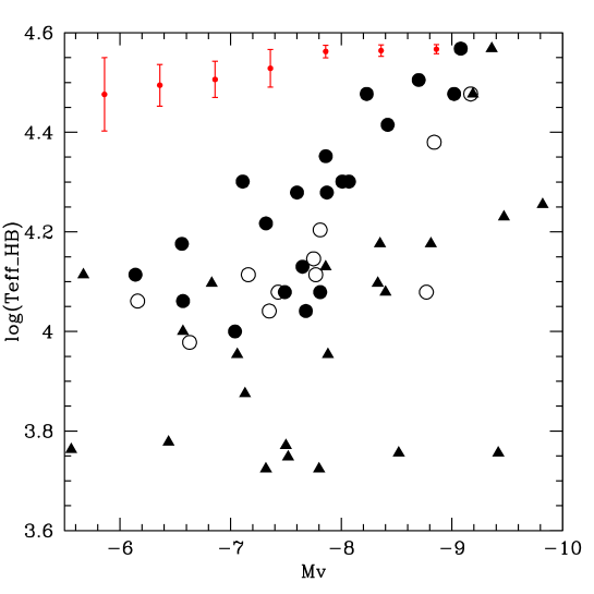
  Figure 4: Upper panel: correlation of log(Teff_HB) with total luminosity, for 3 different metallicity intervals: $[Fe/H]<-1.8$ (open circles), $-1.8<[Fe/H]<-1.3$ (filled circles) and $[Fe/H]>-1.3$ (filled triangles). Points with error bars are measurements from simulated clusters (e.g. the text). Bottom panel: HB morphology-metallicity correlation with different symbol sizes depending on total luminosity, M_V. Note the better correlation of clusters of intermediate luminosity. The smallest clusters ( M${}_{V}>$ -7.8 ) do not reach the bluest HB morphologies, and they all have log(Teff_HB) $<$ 4.35.

• Total luminosity

  Probably one of the most interesting results of this simple correlation approach is the finding of a clear correlation between HB morphology and total luminosity of the cluster. If no selection in metallicity is performed, this correlation is apparently slightly lower than the one observed with the first parameter. The Pearson coefficient relating these two variables is r $\simeq$ -0.48 and therefore, the variation of total luminosity would be responsible for the 23% of the HB morphology variation. However, if only intermediate metallicity clusters are considered, the correlation between log(Teff_HB) and M_V is as high as r $\simeq$ -0.77 (60 % of the total variation). Therefore, the influence of cluster total luminosity on the HB temperature extension seems more important than that of [Fe/H] at this metallicity regime!

  Graphically, this effect is shown in Figure 4, upper panel, where the correlation of log(Teff_HB) with total luminosity for 3 different metallicity intervals is presented. More luminous clusters, tend to have hotter (bluer) horizontal branches. The rms of a linear regression between both quantities is 0.20. On the other hand, if we calculate the Pearson coefficient between total luminosity and log(Teff_HB) only for the subsample of clusters with the more extended HBs, log(Teff_HB) $>$ 4.3, we find a much clearer correlation, reaching a value of r$=$ -0.81. This means that two thirds of the variation in the HB temperature extension can be explained by the variation of M_V for clusters with extreme blue horizontal branches. Bottom panel of Figure 4 shows again the trend of log(Teff_HB) with metallicity, but using different point sizes depending on the value of the total luminosity. Clearly, some of the dispersion in the first parameter correlation can be explained by M_V. That is the case of the metal-rich blue tail clusters NGC6388 and NGC6441, which have M_V $<$ -9, and are among the most luminous clusters in the sample.

  Luminosity is perhaps the most fundamental observed quantity characterizing a stellar system, and for a set of old stellar systems it is a good relative measure of its baryonic mass. Therefore, the observed trend seems to suggest that, for some reason, more massive clusters tend to have bluest horizontal branches. We will come back to this point in Section 7, where we will discuss its possible theoretical implications.

  On the other hand, correlation between HB morphology and total luminosity was previously noted by Fusi Pecci et al. (1993). However, they interpreted this result as a consequence of the high HB morphology-cluster density correlation derived from their analysis. In this paper, we have chosen a different characterization of cluster HB, the maximum temperature extension, which shows a weak correlation with cluster density or even stellar collisions, as we will see later in this Section.

  Finally, we have explored the possibility that the Teff_HB-M_V dependence could be a statistical effect, that is, the higher the number of stars in the cluster (and thus the more massive the cluster is) the higher the probability of finding hot HB stars. The so called “second parameter” could also be a mechanism with a low percentage of incidence, that would be only detected with high enough statistics. In principle, if this were true, we would expect the hot HB stars to be always a small percentage of the total number of HB stars, which is not always the case (see for example the cluster NGC6205). Nevertheless, in order to check the influence of statistics on the M_V parameter dependence, we have performed the following test: we have taken the photometry of one of the most massive clusters in the sample, NGC 2808 (M${}_{V}=-9.36$), whose extremely extended HB reaches a temperature of log(Teff_HB)$=$4.568. The absolute total magnitude of the cluster was then reduced artificially by subtracting the corresponding percentage of stars from the photometry file, using a random selection procedure. Between the 34% and the 96% of the stars were removed for magnitude reductions between 0.5 mag and 3.5 mag. From the resulting simulated CMDs, the highest temperature of the HB was measured following the same technique applied to the real clusters (see Section 3.1). This procedure was repeated 20 times for each simulated cluster magnitude. The results obtained are plotted in Figure 4, upper panel, where the points with error bars correspond to the mean log(Teff_HB) value obtained for each cluster magnitude and its scatter. From our simulations, the HB temperature extension seems to decrease very little as cluster magnitude decreases (less than a 4% in all the magnitude range). On the contrary, the tendency for real clusters (points without error bars in Fig. 4), seems to indicate a steeper decrease of log(Teff_HB) with M_V. Therefore, the performed test proves that the role of statistics in the dependence of HB temperature extension on cluster magnitude is very small. The origin of the log(Teff_HB)-M_V correlation could be a different physical cause, whose possible interpretation will be discussed later (cf. Section 7).

• Collisional parameter

  Figure 5: Correlation of log(Teff_HB) with (from upper left to bottom right) collisional parameter, central density and Galactocentric distance. Symbols indicate different $[Fe/H]$ ranges, as in Figure 4.

  

  Figure 6: Correlation of log(Teff_HB) with globular cluster relative age. Symbols are the same as in Fig. 4 The derived Pearson correlation coefficient is r$=$ 0.04 when all the clusters are considered, but it increases up to r$=$0.76 if only intermediate clusters (filled circles) are taken into account.

  Quite interesting is also the result for the collisional parameter. The correlation between log(Teff_HB) and the $\Gamma_{col}$ is very low and probably inside the errors (r$\simeq$0.14, about 2% of the total HB morphology variance). This value increases up to r$\simeq$0.29, 8% of the total variance, if only intermediate metallicity clusters are considered.

  The relation between log(Teff_HB) and $\Gamma_{col}$ is graphically presented in Figure 5, on the upper left panel. This result seems to suggest that even if the probability of stellar collisions is higher, the HB morphology is not affected. Close encounters and tidal stripping, suggested by Fusi Pecci et al.  (1993) as a possible origin of bluer HB stars, do not seem to have a relevant role in HB morphology. Nevertheless, it is important to note that the collision rate may have varied greatly through the clusters life time, especially in clusters which have undergone core collapse and re-expansion, and/or gravothermal oscillations. Although none particular correlation for core-collapse clusters in the sample has been noted, we should warn about the risk of overinterpreting the lack of a good correlation between log(Teff_HB) and $\Gamma_{col}$.

• Central density

  The scenario is very similar to that inferred from the log(Teff_HB) - $\Gamma_{col}$ correlation. Figure 5, bottom left panel shows the trend of HB temperature extension with the central density of the cluster. Our analysis indicates a weak correlation between both quantities: r$\simeq$0.16 for the complete clusters sample, and r$\simeq$0.30, at intermediate metallicity [2.6% and 9.0% of the total log(Teff_HB) variance respectively]. Again, contrary to previous studies (Fusi Pecci et al.  1993), our sample indicates that cluster density is not a “good” second parameter, as it has a little influence on HB morphology. Nevertheless, an equivalent caveat to that of $\Gamma_{col}$ applies here. The central density now may not be as relevant as the maximum density achieved in the past.

• Other simple correlations

  Other quantities with which HB morphology seems to have a little but, maybe still significant correlations are the distance to the Galactic center, R_GC (r$\simeq$0.19, 4% of the total log(Teff_HB) variance) and half-light radius (r$\simeq$0.18, 3%). The first one, may also be a secondary effect of the first parameter, as $[Fe/H]$ has an already known trend with R_GC.

• Age

  Finally, we have evaluated the influence of cluster age in a subsample of 47 clusters, in common with the De Angeli et al. (2005) data base (see Table 1 and Figure 6). The relative ages of the 47 clusters go from 0.74 $\pm$ 0.06 for the youngest cluster in the sample (NGC 362) to 1.085 $\pm$ 0.06 for the oldest one (NGC 7099). These relative ages are normalized to the average age of the most metal poor clusters ($[Fe/H]<-1.7$) as explained by De Angeli et al. The derived Pearson correlation coefficient between log(Teff_HB) and age is r$=$ 0.04 (0.2% of the HB morphology variance of the clusters subsample). This result confirms the fact, already pointed out by Rosenberg et al. (1999), that age can not be the only explanation for the second parameter problem.

  In general, cluster age most important dependences are those with metallicity (r$=$ 0.38, 14%) and Galactic latitude (r$=$ 0.42, 18%).

  However, it is interesting to point out that if we only consider intermediate metallicity clusters (filled circles in Fig. 6), the correlation between log(Teff_HB) and cluster age increases to r$=$0.76 (58%). This will be explored later in more detail.

5 The multivariate approach.

While the simple approach of examining individual monovariate correlations of log(Teff_HB) with cluster parameters gives us a good first look at the problem of HB morphology, the complexity of the situation calls for a more sophisticated strategy. We are dealing with a multidimensional data set, in which sets of several observables may be connected in multivariate correlations. Simple, monovariate correlations are only a special and rare case. In particular, the different trends of log(Teff_HB) illustrated above indicate that the problem of GC horizontal branch morphology is intrinsically statistically multidimensional, and that must be attacked using a multivariate approach.

First of all, we performed the Principal Component Analysis (PCA) on our data set, using all independent input variables. A code developed at the Instituto de Astrofísica de Canarias (IAC) by A. Aparcio has been used. We ignored the derived quantities, $\rho_{0}$, t_rc, t_rh, as they do not add to the dimensionality of the data manifold. In addition, among the three positional variables R_GC, l and b, we have selected only R_GC and b. In the same way, among the group of variables formed by $\Gamma_{col}$, $\mu_{V}$ and r_c, we took only $\Gamma_{col}$, as it contains the other two parameters in its formula. The input data were renormalized by subtracting the mean and dividing by the sigma in each of the input variables. The number of the significant eigenvalues, i.e., those larger than expected from the measurement errors, gives the dimensionality of the data manifold. Each of the eigenvectors also accounts for a fraction of the total sample variance. It is generally agreed that eigenvalues $>$1 are statistically significant, but somewhat lower ones may be as well, depending on how the data were normalized.

Table 4 presents the eigenvalues (e_i), fractional (V_i) and cumulative (C_i) contributions to the total sample variance, in percent, for the obtained PCA solution. Figure 7 shows the results of the PCA, as applied to the entire above set of independent input variables, in the form of correlation-vector diagrams. Usually, a steep drop in the successive eigenvalues or in the fractional contributions to the sample variance indicates where the number of statistically significant dimensions stops, and where the noise begins. Nevertheless, the situation is not always so clearcut. In this data set, there could be at least four, but probably as many as six statistically significant dimensions or more.

The first four eigenvectors account for the 78.8% of the total sample variance. They define a natural coordinate system for this data set. Projections of the input axes to the principal planes given by the eigenvectors ($\xi_{1},\xi_{2}$) and ($\xi_{1},\xi_{3}$) are the correlation-vector diagrams as shown in Figure 7. In this representation, vectors corresponding to well-correlated variables define sharp or plane angles, on the contrary, uncorrelated quantities have orthogonal vectors.

On the other hand, as in the previous Section, the situation for intermediate metallicity clusters was also considered, by performing PCA computations for the above described 8-parameters, including only clusters with -1.8 $<$ [Fe/H] $<$ -1.3. In that case, the 100% of the data variability is explained with only 7 eigenvalues (the first four eigenvalues account for the 82.8%), thus reflecting the dimensionality decrease.

i	ei	Vi	Ci
1	2.32	29.0	29.0
2	1.85	23.1	52.1
3	1.18	14.8	66.9
4	0.95	11.9	78.8
5	0.71	8.9	87.7
6	0.61	7.6	95.3
7	0.22	2.7	98.0
8	0.16	2.0	100.0

Table 4: Eigenvalues (e_i), fractional (V_i) and cumulative (C_i) contributions to the total sample variance, in percent, for the obtained PCA solution for the set of 8 input independent parameters.

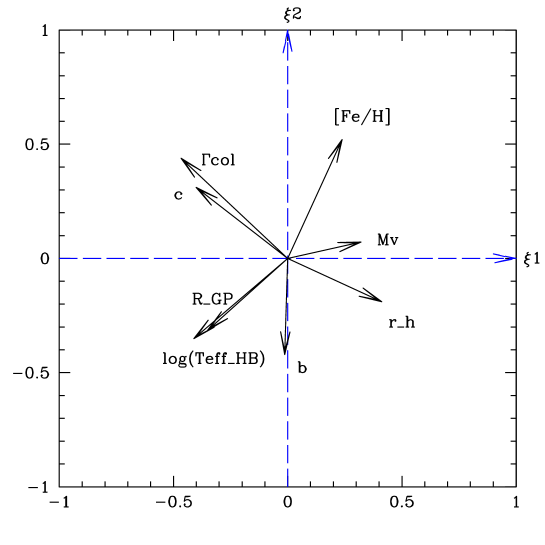
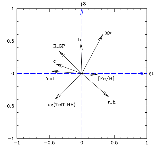
Figure 7: Projections of the input axes to the principal planes given by the eigenvectors ($\xi_{1},\xi_{2}$) and ($\xi_{1},\xi_{3}$).

Obviously, the situation is quite complex, reflecting the statistical multidimensionality of the entire manifold of globular cluster properties (e.g. Djorgovski & Meylan, 1994). Given the limited data set, a more profitable approach is to consider only a subset of variables. To illustrate the point, we will consider only log(Teff_HB), $[Fe/H]$ and M_V. We find that for this data subset of three input variables (see Table 5), at least two statistical dimensions are necessary. The first two eigenvectors account for the 56% and the 34% of the total sample variance, respectively. The remaining 10% could be accounted by the errors, which are quite difficult to evaluate as explained in the previous sections. If this is true, a weighted vector sum of $[Fe/H]$ and M_V vectors could correlate much better with log(Teff_HB) than $[Fe/H]$ or M_V alone. This is shown in Figure 8 where the bivariate correlation involving these 3 input quantities is:

$log$(Teff_HB) $=-0.17\cdot$[Fe/H]$-0.136\cdot$ M${}_{V}+2.84$

Clearly, the dispersion (rms$=$0.16) is now smaller than the one observed in any of the monovariate correlations for the total cluster sample. This bivariate correlation works specially well for clusters with log(Teff_HB) $>$ 3.8 (Teff${}_{HB}\geq$ 6000 K), that is, clusters with at least some blue HB stars. In fact, if we perform the previous bivariate analysis considering only these clusters, we find a much clear correlation, with an rms$=$0.13, as shown in Figure 9 ( we warn however of the smaller quantity of data in Fig 9).

Figure 8: Bivariate correlation involving the variables log(Teff_HB), $[Fe/H]$ and M_V. The solid line is the least square fit to the data. Symbols are those of Fig. 4

i	ei	Vi	Ci
1	1.68	56.0	56.0
2	1.01	33.7	89.7
3	0.31	10.3	100.0

Table 5: PCA solutions for a subsample of 3 parameters : log(Teff_HB), $[Fe/H]$ and M_V.

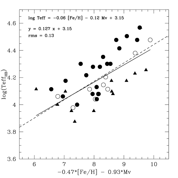
Figure 9: Bivariate correlation of HB morphology with optimized combinations of $[Fe/H]$ and M_V for clusters with log(Teff_HB) $>$ 3.8. The plotted lines are the least square fit to the included data (solid) and to clusters with $[Fe/H]\leq-1.3$ (dashed). Symbols are those of Fig. 4

.

On the other hand, we have also explored the trivariate correlation of HB morphology with $[Fe/H]$, M_V and Age in order to possibly reduce the scatter in the previous bivariate relation, due to possible effects of age. The analysis was performed for a subsample of the 47 clusters in common with De Angeli et al. (2005) which had $[Fe/H]<-1.3$. The corresponding PCA results are presented in Table 6 and Figure 10. The third eigenvector significance, 14.8%, increases with respect to the combination of $[Fe/H]$ and M_V. Now, the first three eigenvectors account for the 93.0 % of the total variance. The residual scatter is, therefore, of the order of the measurement errors.

i	ei	Vi	Ci
1	1.86	46.5	46.5
2	1.21	30.2	76.7
3	0.69	17.3	94.0
4	0.24	6.0	100.0

Table 6: PCA solutions for the subsample of 4 parameters : log(Teff_HB), $[Fe/H]$, M_V and Age.

Figure 10: Trivariate correlations of HB morphology with optimized combinations of $[Fe/H]$, M_V and Age for a subsample of 28 clusters in common with De Angeli et al. (2005) and $[Fe/H]\leq-1.3$. Symbols are those of Fig. 4

6 Summary and discussion: theoretical implications.

In this section, the results of the multivariate analysis presented above are summarized, trying to shed some light in their possible theoretical meaning.

As it has been extensively discussed by Djorgovski et al. (1993) the GC manifold is rather complex, and this is perfectly true also when we focus our attention on the problem of the GC HB morphology and of its dependence on the cluster parameters. In the previous section, we have shown that at least four parameters, but probably up to eight, are needed to reproduce the HB extension in temperature. As Fusi Pecci, Buonnanno and collaborators (see for example Fusi Pecci et al,̇ 1993), among others, have been remarking in the last 20 years or so, there is no single “second parameter” which can explain the HB anomalies, but a combination of parameters.

The present analysis, based on 54 GCs of the HST snapshot catalogue, has given a few interesting new results which are worth of further discussion.

At least one new interesting conclusion can be derived: the importance of total cluster luminosity, and therefore of total mass, on the horizontal branch morphology. This effect, combined with the first parameter, can explain probably the major part of the Galactic globular cluster horizontal branch morphologies. More massive clusters (i.e. more luminous) tend to have more extended horizontal branches. To this scenario, we have to add the effect of age, evaluated here for 47 clusters in common with De Angeli et al. (2005). Lastly, the situation for intermediate-metallicity clusters has also been analysed, leading to a higher correlation between the temperature extension of the HB and M_V (60% of the total variation), with small increments of the $\Gamma_{col}$ and the central density contributions, that remain nevertheless inferior to 9%.

One possible interpretation to the considerable influence of M_V and therefore, of cluster total mass, on HB morphology can be derived from the paper by D’Antona et al.  2002. They analyze the consequences, on HB morphology, of helium variation due to self-pollution among globular cluster stars. Self-pollution had already been proposed as an explanation for the chemical inhomogeneities (spread in the abundances of CNO, O - Na and Mg anticorrelation) observed in GC members from the main sequence to the RGB (see for example Gratton et al. 2001). The ejecta of massive asymptotic giant branch stars, which would be the origin of the self pollution, would not only be CNO processed, but also helium enriched. D’Antona et al.  (2002) models take into account this possible helium enhancement with respect to the primordial value. They find that a spread in the helium content does not affect the morphology of the main sequence, turn off and RGB in an easily observable way. However, the difference in the evolving mass may play a role in the formation of blue tails, as higher helium stars would be able to populate much bluer HB regions. If this is correct, self-pollution and so helium enrichment would be higher in more massive clusters, as they would be able to retain the material from the ejecta better than less massive clusters.

As already pointed out by Rosenberg, Recio-Blanco & García-Marín (2004), M54, believed to be the remaining core of the Sagittarius dwarf galaxy could be another example of this scenario. More recently, the abundance analysis of stars in the double main sequence of $\omega$ Centauri (Piotto et al., 2005) suggests the presence of two populations of stars, one of which is strongly He enhanced. This could be another observational indication supporting the D’Antona et al. theory in a very massive cluster.

Finally, whatever is the theoretical interpretation of the data, a clear conclusion of this analysis is that the influence of M_V on HB extension seems to be as important as those of metallicity and age. Cluster total mass must be playing an important role in horizontal branch morphology.