Principal Component Analysis of Weak Lensing Surveys

Abstract

Aims. We study degeneracies between cosmological parameters and measurement errors from cosmic shear surveys. We simulate realistic survey topologies with non-uniform sky coverage, and quantify the effect of survey geometry, depth and noise from intrinsic galaxy ellipticities on the parameter errors. This analysis allows us to optimise the survey geometry.

Methods. We carry out a principal component analysis of the Fisher information matrix to assess the accuracy with which linear combinations of parameters can be determined. Using the shear two-point correlation functions and the aperture mass dispersion, which can directly be measured from the shear maps, we study various degeneracy directions in a multi-dimensional parameter space spanned by $\Omega_{\rm m}$, $\Omega_{\Lambda}$, $\sigma_{8}$, the shape parameter $\Gamma$, the spectral index $n_{\rm s}$, along with parameters that specify the distribution of source galaxies.

Results. A principal component analysis is an effective tool to probe the extent and dimensionality of the error ellipsoid. If only three parameters are to be obtained from weak lensing data, a single principal component is dominant and contains all information about the main parameter degeneracies and their errors. For four or more free parameters, the first two principal components dominate the parameter errors. The degeneracy directions are insensitive against variations in the noise or survey geometry. The variance of the dominant principal component of the Fisher matrix, however, scales with the noise. Further, it shows a minimum for survey strategies which have small cosmic variance and measure the shear correlation up to several degrees. This minimum is less pronounced if external priors are added, rendering the optimisation less effective. The minimisation of the Fisher error ellipsoid can lead to slightly different results than the principal component analysis.

1 Introduction

Recent observations by the Wilkinson Microwave Anisotropy Probe (WMAP) mission confirmed the standard cosmological model with a very high degree of accuracy (Spergel et al. 2003). In particular, these observations confirmed that the universe is spatially flat and dominated by dark energy and dark matter. Regarding the initial power spectrum of scalar perturbations, the predictions of the simplest inflationary models were strengthened, i.e. the near scale-invariance, adiabaticity and Gaussianity of the initial density perturbations. However, certain outstanding issues remain to be solved, such as the running of spectral index $\alpha_{\rm s}$ which can be addressed in more detail with additional data from galaxy surveys such as SDSS (York et al. 2000), 2dF (Colless et al. 2001) and the Lyman-$\alpha$ forest (see Seljak et al. 2003 and references therein).

Weak lensing surveys are expected to make important and complementary contributions to high-precision measurements of cosmological parameters. Contaldi et al. (2003) used the Red Cluster Sequence (RCS) to show that the $\Omega_{\rm m}$-$\sigma_{8}$ degeneracy direction is nearly orthogonal to the one from CMB measurements, making weak lensing particularly suitable for combined analyses (van Waerbeke et al. 2002). Ishak et al. (2003) argued that a joint CMB-cosmic shear survey provides an optimal data set for constraining the amplitude and running of spectral index which helps to probe various inflationary models. Tereno et al. (2004) studied cosmological forecasts for joint CMB and weak lensing data. Clearly, the potential of weak lensing surveys (Mellier 1999; Bartelmann & Schneider 2001; Réfrégier 2003; van Waerbeke & Mellier 2003; Schneider 2005) as a cosmological probe is now well established (Contaldi et al. 2003; Hu & Tegmark 1999). In the last few years there have been many studies which have detected cosmic shear in random patches of the sky (Brown et al. 2003; Bacon et al. 2003; Bacon, Réfrégier & Ellis 2000; Hamana et al. 2003; Hämmerle et al. 2002; Hoekstra et al. 2002a; Hoekstra, Yee & Gladders 2002a; Jarvis et al. 2002; Kaiser, Wilson & Luppino 2000; Maoli et al. 2001; Réfrégier, Rhodes, & Groth 2002; Rhodes, Réfrégier & Groth 2001; van Waerbeke et al. 2000, 2001, 2002; Wittman et al. 2000). While early studies were primarily concerned with the detection of the weak lensing signal, present generations of weak lensing observations are putting constraints on cosmological parameters, in particular the matter density parameter $\Omega_{\rm m}$ and the power spectrum normalisation $\sigma_{8}$.

Inspired by the success of these surveys, there are many other ongoing, planned and proposed weak lensing surveys which are currently in progress, including the Deep Lens Survey (Wittman et al. 2002), the Canada-France-Hawaii Telescope Legacy Survey (Hoekstra et al. 2005; Semboloni et al. 2005), the Panoramic Survey Telescope and Rapid Response System, the Supernova Acceleration Probe (Massey et al. 2003), the NOAO Deep Wide-Field Survey (Groch et al. 2002) and the Large Synoptic Survey Telescope (Tyson et al. 2002). Future cosmic shear surveys will be able to probe much larger scales in the linear regime which will provide more stringent bounds on cosmological parameters such as the equation of sate of dark energy and its time variations.

In a recent work (Kilbinger & Schneider 2004, hereafter KS04), the impact of the survey design on cosmological parameter constraints was analysed using a likelihood and Fisher matrix analysis, extending previous studies based on the assumption of uniform sky coverage (Schneider et al. 2002a). Earlier work in this direction by Kaiser (1998) considered a singe $3^{\circ}\times 3^{\circ}$ -field and studied the effect of sparse sampling and intrinsic ellipticity dispersion. The motivation for the present work remains the same, although we concentrate on the eigenvalues of the Fisher matrix. Therefore, in contrast to KS04 where the 1$\sigma$ errors on individual parameters have been used to optimise the survey geometry, we consider all parameter combinations corresponding to the eigenvectors of the Fisher matrix. We study how noise due to the intrinsic ellipticity dispersion of galaxies $\sigma_{\epsilon}$, the number density of galaxies $n_{\rm gal}$, the survey depth and marginalisation affects the determination of the parameter combinations for various survey strategies.

Cosmic shear is sensitive to a large number of cosmological parameters. However, the dependency on these parameters is partially degenerate (although these degeneracies can be broken by the use of external data sets such as CMB, galaxy surveys and Lyman-$\alpha$ surveys). A principal component analysis (PCA) can be used as an efficient tool to identify the degeneracy directions and linear combinations of cosmological parameters, rank-ordered according to the accuracy with which they can be determined from a given survey set-up. Indeed, in recent years there has been a renewed interest in applying principal component analysis techniques to various cosmological data sets, a technique pioneered by Efstathiou & Bond (1999). This method can reveal the detailed statistical structure of cosmological parameter space which is lacking in an one-dimensional confidence level presentation. Efstathiou (2002) studied PCA in the context of the tensor degeneracy in CMB. For a recent work see Rocha et al. (2004), where the possibility of measurement of the fine-structure constant $\alpha$ has been explored in the context of CMB data with analysis based on Fisher matrix and PCA. Hu & Keeton (2002) applied this technique to map the density distribution along the radial direction from weak lensing surveys. Jarvis & Jain (2004) used PCA to correct for the point spread function (PSF) variation in weak lensing surveys. In the context of SN Ia observations to constrain the dark energy equation of state, Huterer & Starkman (2003) and Huterer & Cooray (2004) employed PCA and its variants (see Wang & Tegmark 2005; Crittenden & Pogosian 2005 for more recent results). Tegmark et al. (1998) used PCA for decorrelating the power spectrum of galaxies. This idea was initially proposed by Hamilton (1997) and further discussed in the context of galaxy surveys by Hamilton & Tegmark (2000).

This paper is organised as follows: in Sect. 2, a very brief overview of our notations is provided; in particular, we introduce how the covariance matrix and the Fisher matrix is constructed for a given estimator and a given survey strategy. This section also outlines the basics of principal components analysis. In the next section (Sect. 3) we provide the details of survey geometries and the numerical results of the PCA considering three survey set-ups. For a small number of cosmological parameters, ($\leq 4$) we consider various survey strategies and try to optimise those. For a larger set of parameters, we consider a ten times larger shear survey. Effects of various noise sources on the principal components are investigated. Section 4 is left for discussions and future prospects.

2 Notation and formalism

2.1 Second-order shear statistics

In our numerical studies presented here, we use the two-point correlation functions of shear $\xi_{\pm}$ and the aperture mass dispersion $\langle M_{\rm ap}^{2}\rangle$ to predict constraints on cosmological parameters. Both these statistics depend linearly on the convergence power spectrum $P_{\kappa}$ (Kaiser 1992; Kaiser 1995; Schneider 1996; Schneider et al. 1998)

$$\xi_{\pm}(\theta) = \frac{1}{2\pi}\int\limits_{0}^{\infty}{\mathrm{d}}\ell\,\ell\,P_{\kappa}(\ell){\rm J}_{0,4}(\ell\theta);$$

$$\left\langle M_{\rm ap}^{2}(\theta)\right\rangle = \frac{1}{2\pi}\int\limits_{0}^{\infty}{\mathrm{d}}\ell\,\ell\,P_{\kappa}(\ell)\left(\frac{24\,{\rm J}_{4}(\ell\theta)}{(\ell\theta)^{2}}\right)^{2},$$ (1)

where ${\rm J}_{\nu}$ is the first-kind Bessel function of order $\nu$.

Estimators of these statistics and their covariances are defined in Schneider et al. (2002a). We use the Monte-Carlo-like method from KS04 to integrate the analytical expressions of the covariances, which are exact in case of a Gaussian shear field. Our result is expected to underestimate the covariance due to non-Gaussian contributions on scales between $\sim$ 1 and 10 arc minutes.

2.2 Fiducial cosmological model

We calculate the convergence power spectrum and the shear estimators using the non-linear fitting formulae of Peacock & Dodds (1996). Our cosmological model has seven free parameters: These are the five cosmological parameters $\Omega_{\rm m}$, $\Omega_{\Lambda}$, the power spectrum normalisation $\sigma_{8}$, the spectral index of the initial scalar fluctuations $n_{\rm s}$ and $\Gamma$, which determines the shape of the power spectrum. The fiducial model is assumed to be a flat $\Lambda$CDM cosmology with $\Omega_{\rm m}=0.3$, $\sigma_{8}=1$, $\Gamma=0.21$ and $n_{\rm s}=1$. The two parameters $z_{0}$ and $\beta$ characterise the redshift distribution of background galaxies (Brainerd et al. 1996),

$$p(z){\rm d}z={\beta\over z_{0}\Gamma(3/\beta)}\left({z\over z_{0}}\right)^{2}e^{-(z/z_{0})^{\beta}}{\rm d}z,$$ (2)

with fiducial values $z_{0}=1$ and $\beta=1.5$.

2.3 Principal components analysis of the Fisher matrix

We use the expression for the Fisher matrix (see Tegmark, Taylor & Heavens 1997 for a review) in the case of Gaussian errors and parameter-independent covariance,

$$F_{ij}=\sum\limits_{ij}\left(\frac{\partial x_{k}}{\partial\Theta_{i}}\right)({\bf C}^{-1})_{kl}\left(\frac{\partial x_{l}}{\partial\Theta_{j}}\right),$$ (3)

where $x_{k}$ is either $\xi_{+}(\theta_{k})$, $\xi_{-}(\theta_{k})$, $\langle M_{\rm ap}^{2}(\theta_{k})\rangle$ or an entry of the combined correlation function $\xi_{\rm tot}=(\xi_{+},\xi_{-})$. ${\bf C}$ denotes the covariance matrix of the estimator of the corresponding shear statistics, $\@vec{\Theta}=(\Theta_{1},\ldots\Theta_{n})$ is the vector of cosmological parameters. The inverse of the Fisher matrix is the covariance of the parameter vector at the point of maximum likelihood,

$${\bf F}^{-1}=\langle\Delta\@vec{\Theta}\Delta\@vec{\Theta}^{\rm t}\rangle=\langle\@vec{\Theta}\@vec{\Theta}^{\rm t}\rangle-\langle\@vec{\Theta}\rangle\langle\@vec{\Theta}^{\rm t}\rangle.$$ (4)

The standard deviation of the $i^{\rm th}$ parameter obtained from the Fisher matrix, $\Delta\Theta_{i}=(\langle\Theta_{i}^{2}\rangle-\langle\Theta_{i}\rangle^{2})^{1/2}=[({\bf F}^{-1})_{ii}]^{1/2}$, is called the minimum variance bound (MVB). According to the Cramér-Rao inequality, the variance of any unbiased estimator is always larger or equal to the MVB.

Any real matrix ${{\bf W}}$ is called a decorrelation matrix if it satisfies

$${{\bf F}}={{\bf W}}^{\rm t}{\bf\Lambda}{\bf W},$$ (5)

where ${\bf\Lambda}$ is a diagonal matrix (Hamilton & Tegmark 2000). The quantities ${\@vec{\Phi}}={\bf W}{\@vec{\Theta}}$ are uncorrelated because their covariance matrix is diagonal,

$$\langle{\Delta\@vec{\Phi}}{\Delta\@vec{\Phi}}^{\rm t}\rangle={\bf W}\langle\Delta\@vec{\Theta}\Delta\@vec{\Theta}^{\rm t}\rangle{\bf W}^{\rm t}={\bf\Lambda}^{-1}.$$ (6)

By multiplying ${\bf W}$ with the square root of the diagonal matrix ${\bf\Lambda}$, the quantities $\@vec{\Phi}$ can be scaled to unit variance without loss of generality. In this case, (5) is written as

$${{\bf F}}=\tilde{{\bf W}}^{\rm t}\tilde{{\bf W}},$$ (7)

where $\tilde{{\bf W}}={{\bf\Lambda}}^{1/2}\,{\bf W}$. Note that the choice of $\tilde{{\bf W}}$ is not unique. If some matrix $\tilde{{\bf W}}$ satisfies (7), the same is true for any orthogonal rotation ${\bf O}\tilde{{\bf W}}$ with ${\bf O}\in{\rm SO}(n)$ and therefore, there are infinitely many decorrelation matrices satisfying (7).

If ${\bf W}$ is an orthogonal matrix, its rows are the eigenvectors $\@vec{p}_{i}$ of ${\bf F}$ and ${\bf\Lambda}={\rm diag}(\lambda_{i})$ is the diagonal matrix of the corresponding eigenvalues. In that case, (5) is called a principal component decomposition. We assume the eigenvalues to be in descending order.

The eigenvectors or principal components of ${\bf F}$ determine the principal axes of the $n$-dimensional error ellipsoid in parameter space. The eigenvectors represent orthogonal linear combinations of the physical (cosmological) parameters that can be determined independently from the data. The more these vectors are aligned with the parameter axes, the less are the degeneracies between those parameters. The accuracy with which these linear parameter combinations can be determined is quantified by the variance $\sigma_{i}\equiv\sigma(\@vec{p}_{i})=\Delta\Phi_{i}=\Lambda_{ii}^{-1/2}=\lambda_{i}^{-1/2}$. Thus, a principal component decomposition of the Fisher matrix gives us information about which (linear) parameter combinations can be determined with what accuracy from a given data set. Since the eigenvalues are in descending order, the first eigenvector $\@vec{p}_{1}$ having the smallest variance corresponds to the best constrained parameter combination. The last eigenvector $\@vec{p}_{n}$ is the direction with the largest uncertainty.

From (6), one can calculate the MVB from the eigenvectors and eigenvalues of ${\bf F}$,

$$\Delta\Theta_{j}=\left(\sum_{i=1}^{n}W_{ji}^{2}\,\lambda_{i}^{-1}\right)^{1/2}.$$ (8)

3 Numerical results

3.1 Survey strategies

We simulate shear surveys consisting of $P$ circular, uncorrelated patches of radius $R$ on the sky, each in which $N$ individual fields of view of size $13^{\prime}\times 13^{\prime}$ are distributed randomly but non-overlapping. The total number of fields of view is $n=PN=300$, corresponding to a total survey area of $A=14.1$ square degree. Different surveys with $N=$ 10, 20, 30, 50, and 60 are considered, corresponding to geometries with $P=$ 30, 15, 10, 6 and 5 patches, respectively (see KS04).

We denote these survey strategies with $(N,R)$, e.g. $(50,100^{\prime})$ corresponds to a survey with $N=50,R=100^{\prime}$ and $P=6$. Further, we consider a survey consisting of 300 uncorrelated lines of sight à $13^{\prime}\times 13^{\prime}$, which are randomly distributed on the sky. This survey, denoted by $300\cdot 13^{\prime\,2}$, has smaller cosmic variance than any of the patch strategies, but does not sample intermediate and large angular scales.

If not indicated otherwise, the number density of source galaxies is $n_{\rm gal}=30\,{\rm arcmin}^{-2}$. This number density of high-redshift galaxies which are usable for weak lensing shape measurements can be achieved with high-quality ground-based imaging data on a 4 m-class telescope. The source galaxy ellipticity dispersion is $\sigma_{\varepsilon}=0.3$, if not stated otherwise. For comparison, these quantities are varied to $n_{\rm gal}=20$ and $40\,{\rm arcmin}^{-2}$, and $\sigma_{\varepsilon}=0.2,0.4$, respectively, to study the effect of noise sources on the principal components.

3.2 Eigenvalues of the Fisher matrix

We consider the Fisher matrix ${\bf F}$ corresponding to all seven cosmological and redshift parameters. In this section, we demonstrate the influence of survey characteristics (other than the geometry) on the eigenvalues $\lambda_{i}$ of ${\bf F}$. The variance of the linear combination of parameters given by the $i^{\rm th}$ eigenvector $\@vec{p}_{i}$ of ${\bf F}$ is $\sigma(\@vec{p}_{i})=\lambda_{i}^{-1/2}$, as defined in Sect. 2.3. In Fig. 1 we show the effect of the number of background galaxies, $n_{\rm gal}$, and the intrinsic ellipticity dispersion, $\sigma_{\varepsilon}$. In both cases, the noise variation causes a scaling of the variance. For the intrinsic ellipticity dispersion, the scaling factor increases with $i$. The $i=1$ variance scales linearly with $\sigma_{\varepsilon}$, whereas the mean dependence (averaged over all 7 eigenvalues) is quadratic in $\sigma_{\varepsilon}$. In the case of $n_{\rm gal}$, however, the variance $\sigma_{i}$ of all eigenvectors is scaled by a constant factor which is inversely proportional to $n_{\rm gal}$. The variance of the eigenvectors are steeper functions of the noise characteristics than the MVB (Kilbinger & Munshi 2005). Note however, that in this previous study the MVB was calculated for each parameter individually, without taking parameter correlations into account.

If boundary effects due to the finite field of the survey are neglected, the covariance is anti-proportional to the observed survey area. Consequently, the variance $\sigma_{i}$ scales as $f_{\rm sky}^{-1/2}$, where $f_{\rm sky}$ is the fractional sky coverage of the survey. As an example, we compare the $300\cdot 13^{\prime\,2}$ survey with a survey consisting of 50 patches with $N=60$ and $R=140^{\prime}$ (corresponding to ten $(60,140^{\prime})$ surveys). We found a good agreement on the expected scaling of $\sigma_{i}$ as a function of the survey area, although for the combinations which are worst constrained by the data, the dependence on $f_{\rm sky}$ seems to be steeper (see Fig. 2).

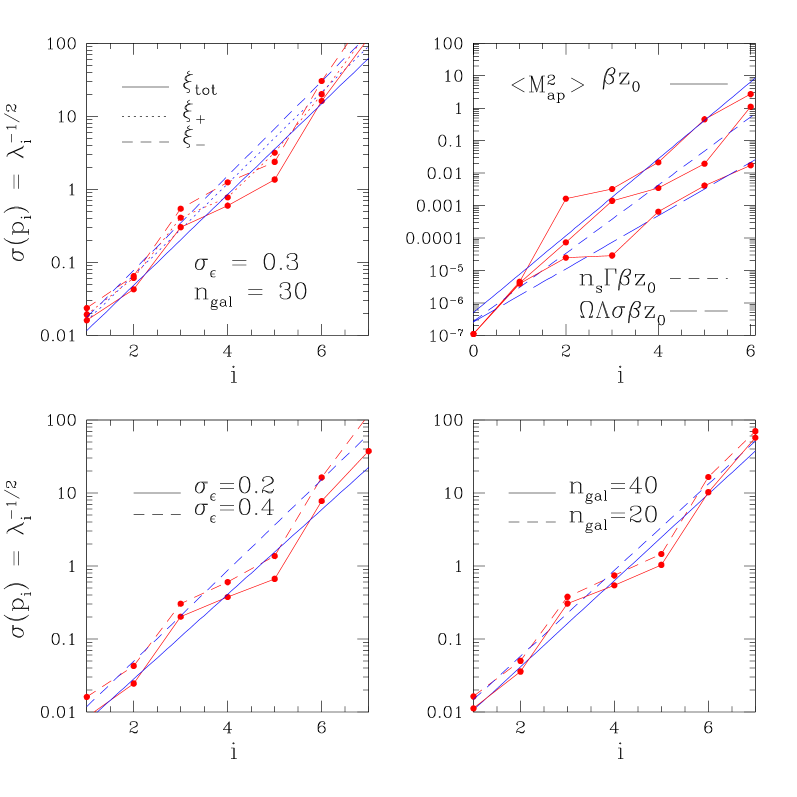
Figure 1: The variance $\sigma(\@vec{p}_{i})=\lambda_{i}^{-1/2}$ associated with the principal components of the 7$\times$7 Fisher matrix. The straight lines are fits to the data points. Lower left panel: $\sigma(\@vec{p}_{i})$ as a function of the intrinsic ellipticity dispersion of galaxies $\sigma_{\varepsilon}=0.2$ and 0.4. Lower right: the variation of $\sigma(\@vec{p}_{i})$ with the number density of galaxies $n_{\rm gal}=20$ and 40. Upper left: the variation of $\sigma(p_{n})$ for three different estimators, $\xi_{+}$, $\xi_{-}$ and $\xi_{tot}$. Upper right: the variation of $\sigma(\@vec{p}_{i})$ for three different priors, see Sect. 3.11. The survey strategy is $(30,100^{\prime})$ in all cases.

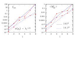
Figure 2: The variation of $\sigma(\@vec{p}_{i})$ as a function of the eigenvector number $i$, for $\xi_{\rm tot}$ (left panel) and $\langle M^{2}_{\rm ap}\rangle$ (right panel). The redshift parameter $\beta$ is fixed, and a Gaussian prior with variance $s(\sigma_{8})=0.1$ is added to regularise the Fisher matrix. Two surveys with size $14.1$ (solid lines) and 141 square degree (dashed), respectively, are displayed.

3.3 Eigenvectors of the Fisher matrix

In Tables 1–6, the eigenvectors of the Fisher matrix corresponding to various combinations of parameters are shown, for the 2PCF and the aperture mass dispersion.

Table 1: Eigenvectors of the Fisher matrix corresponding to ($\Omega_{\rm m}$, $\Gamma$, $\sigma_{8}$) and a flat Universe as prior, for $\langle M_{\rm ap}^{2}\rangle$ using the survey strategy $(50,100^{\prime})$. $\lambda_{i}^{-1/2}=\sigma_{i}$ is the variance of the $i^{\rm th}$ eigenvector, $\Theta_{j}$ the MVB for the $j^{\rm th}$ cosmological parameter.

	$\@vec{p}_{1}$	$\@vec{p}_{2}$	$\@vec{p}_{3}$	$\triangle\Theta_{j}$
$\Omega_{\rm m}$	$0.649$	$-0.533$	$-0.542$	$0.165$
$\Gamma$	$0.563$	$\phantom{-}0.816$	$-0.128$	$0.042$
$\sigma_{8}$	$0.511$	$-0.222$	$\phantom{-}0.830$	$0.252$
$\lambda_{i}^{-1/2}$	$0.004$	$\phantom{-}0.020$	$\phantom{-}0.300$

Table 2: Eigenvectors of the Fisher matrix corresponding to ($\Omega_{\rm m}$, $\Gamma$, $\sigma_{8}$, $n_{\rm s}$) and the prior $\Omega_{\Lambda}=0.7$, for $\langle M_{\rm ap}^{2}\rangle$ using the survey strategy $(50,100^{\prime})$.

	$\@vec{p}_{1}$	$\@vec{p}_{2}$	$\@vec{p}_{3}$	$\@vec{p}_{4}$	$\Delta\Theta_{j}$
$\Omega_{\rm m}$	0.563	$-0.671$	$\phantom{-}0.322$	$-0.358$	0.254
$\Gamma$	$0.575$	$\phantom{-}0.622$	$-0.235$	$-0.474$	0.333
$\sigma_{8}$	$0.522$	$-0.161$	$\phantom{-}0.501$	$\phantom{-}0.670$	0.473
$n_{\rm s}$	0.281	$\phantom{-}0.368$	$\phantom{-}0.767$	$\phantom{-}0.443$	0.329
$\lambda_{i}^{-1/2}$	$0.004$	$\phantom{-}0.015$	$\phantom{-}0.147$	$\phantom{-}0.698$

Table 3: Eigenvectors of the Fisher matrix corresponding to ($\Omega_{\rm m}$, $\Gamma$, $\sigma_{8}$, $\Omega_{\Lambda}$) for $\langle M_{\rm ap}^{2}\rangle$ using the survey strategy $(50,100^{\prime})$.

	$\@vec{p}_{1}$	$\@vec{p}_{2}$	$\@vec{p}_{3}$	$\@vec{p}_{4}$	$\triangle\Theta_{j}$
$\Omega_{\rm m}$	$\phantom{-}0.587$	$\phantom{-}0.643$	$\phantom{-}0.352$	$-0.341$	$0.169$
$\Gamma$	$\phantom{-}0.591$	$-0.694$	$\phantom{-}0.392$	$\phantom{-}0.114$	$0.112$
$\sigma_{8}$	$\phantom{-}0.542$	$\phantom{-}0.117$	$-0.727$	$\phantom{-}0.404$	$0.252$
$\Omega_{\Lambda}$	$-0.102$	$\phantom{-}0.299$	$\phantom{-}0.439$	$\phantom{-}0.840$	$0.368$
$\lambda_{i}^{-1/2}$	$\phantom{-}0.004$	$\phantom{-}0.015$	$\phantom{-}0.258$	$\phantom{-}0.417$

Table 4: Eigenvectors of the Fisher matrix corresponding to ($\Omega_{\rm m}$, $\Gamma$, $\sigma_{8}$) and a flat Universe as prior, for $\xi_{{\rm tot}}$ ($\xi_{+},\xi_{-}$ in brackets) using the survey strategy $(50,100^{\prime})$.

	$\@vec{p}_{1}$	$\@vec{p}_{2}$	$\@vec{p}_{3}$	$\triangle\Theta_{j}$
$\Omega_{\rm m}$	0.702	$-0.474$	$-0.530$	0.144
	$(0.731)^{+}$	$(-0.435)^{+}$	$(-0.524)^{+}$	$(0.164)^{+}$
	$(0.665)^{-}$	$(-0.515)^{-}$	$(-0.540)^{-}$	$(0.213)^{-}$
$\Gamma$	$0.473$	$\phantom{-}0.868$	$-0.150$	0.043
	$(0.412)^{+}$	$\phantom{-}(0.895)^{+}$	$(-0.167)^{+}$	$(0.056)^{+}$
	$(0.536)^{-}$	$\phantom{-}(0.833)^{-}$	$(-0.134)^{-}$	$(0.057)^{-}$
$\sigma_{8}$	$0.531$	$-0.145$	$\phantom{-}0.834$	0.226
	$(0.542)^{+}$	$(-0.093)^{+}$	$\phantom{-}(0.834)^{+}$	$(0.261)^{+}$
	$(0.519)^{-}$	$(-0.200)^{-}$	$\phantom{-}(0.830)^{-}$	$(0.327)^{-}$
$\lambda_{i}^{-1/2}$	0.004	$\phantom{-}0.017$	$\phantom{-}0.271$
$(\lambda_{i}^{-1/2})^{+}$	$(0.005)^{+}$	$\phantom{-}(0.020)^{+}$	$\phantom{-}(0.313)^{+}$
$(\lambda_{i}^{-1/2})^{-}$	$(0.006)^{-}$	$\phantom{-}(0.027)^{-}$	$\phantom{-}(0.394)^{-}$

Table 5: Eigenvectors of the Fisher matrix corresponding to ($\Omega_{\rm m}$, $\Gamma$, $\sigma_{8}$, $n_{\rm s}$) and the prior $\Omega_{\Lambda}=0.7$, for $\xi_{\rm tot}$ ($\xi_{+},\xi_{-}$ in brackets) using the survey strategy $(50,100^{\prime})$.

	$\@vec{p}_{1}$	$\@vec{p}_{2}$	$\@vec{p}_{3}$	$\@vec{p}_{4}$	$\triangle\Theta_{j}$
$\Omega_{\rm m}$	0.657	$-0.588$	$\phantom{-}0.282$	$-0.376$	0.154
	$(0.708)^{+}$	$(-0.533)^{+}$	$\phantom{-}(0.320)^{+}$	$(-0.332)^{+}$	$(0.158)^{+}$
	$(0.591)^{-}$	$(-0.647)^{-}$	$\phantom{-}(0.329)^{-}$	$(-0.349)^{-}$	$(0.290)^{-}$
$\Gamma$	$0.474$	$\phantom{-}0.719$	$-0.217$	$-0.459$	0.182
	$(0.406)^{+}$	$\phantom{-}(0.768)^{+}$	$(-0.116)^{+}$	$(-0.480)^{+}$	$(0.198)^{+}$
	$(0.547)^{-}$	$\phantom{-}(0.654)^{-}$	$(-0.205)^{-}$	$(-0.480)^{-}$	$(0.389)^{-}$
$\sigma_{8}$	$0.542$	$-0.062$	$-0.474$	$\phantom{-}0.690$	0.279
	$(0.548)^{+}$	$\phantom{-}(0.005)^{+}$	$(-0.572)^{+}$	$\phantom{-}(0.611)^{+}$	$(0.289)^{+}$
	$(0.533)^{-}$	$(-0.129)^{-}$	$(-0.522)^{-}$	$\phantom{-}(0.653)^{-}$	$(0.538)^{-}$
$n_{\rm s}$	$0.217$	$\phantom{-}0.363$	$0.805$	$\phantom{-}0.415$	0.209
	$(0.179)^{+}$	$\phantom{-}(0.352)^{+}$	$\phantom{-}(0.746)^{+}$	$\phantom{-}(0.535)^{+}$	$(0.290)^{+}$
	$(0.257)^{-}$	$\phantom{-}(0.367)^{-}$	$\phantom{-}(0.760)^{-}$	$\phantom{-}(0.470)^{-}$	$(0.414)^{-}$
$\lambda_{i}^{-1/2}$	0.004	$\phantom{-}0.013$	$\phantom{-}0.165$	$\phantom{-}0.389$
$(\lambda_{i}^{-1/2})^{+}$	$(0.005)^{+}$	$\phantom{-}(0.016)^{+}$	$\phantom{-}(0.255)^{+}$	$\phantom{-}(0.408)^{+}$
$(\lambda_{i}^{-1/2})^{-}$	$(0.006)^{-}$	$\phantom{-}(0.020)^{-}$	$\phantom{-}(0.221)^{-}$	$\phantom{-}(0.804)^{-}$

Table 6: Eigenvectors of the Fisher matrix corresponding to ($\Omega_{\rm m}$, $\Gamma$, $\sigma_{8}$, $\Omega_{\Lambda}$), for $\xi_{\rm tot}$ ($\xi_{+},\xi_{-}$ in brackets) using the survey strategy $(50,100^{\prime})$.

	$\@vec{p}_{1}$	$\@vec{p}_{2}$	$\@vec{p}_{3}$	$\@vec{p}_{4}$	$\triangle\Theta_{j}$
$\Omega_{\rm m}$	$\phantom{-}0.676$	$\phantom{-}0.556$	$\phantom{-}0.082$	$-0.475$	0.147
	$\phantom{-}(0.722)^{+}$	$\phantom{-}(0.501)^{+}$	$\phantom{-}(0.030)^{+}$	$(-0.475)^{+}$	$(0.172)^{+}$
	$\phantom{-}(0.613)^{-}$	$(0.619)^{-}$	$\phantom{-}(0.348)^{-}$	$(-0.343)^{-}$	$(0.213)^{-}$
$\Gamma$	$\phantom{-}0.479$	$-0.773$	$\phantom{-}0.385$	$-0.156$	0.094
	$\phantom{-}(0.408)^{+}$	$(-0.808)^{+}$	$\phantom{-}(0.371)^{+}$	$(-0.207)^{+}$	$(0.112)^{+}$
	$\phantom{-}(0.558)^{-}$	$(-0.718)^{-}$	$\phantom{-}(0.400)^{-}$	$\phantom{-}(0.110)^{-}$	$(0.156)^{-}$
$\sigma_{8}$	$\phantom{-}0.555$	$\phantom{-}0.022$	$-0.339$	$\phantom{-}0.759$	0.244
	$\phantom{-}(0.556)^{+}$	$(-0.039)^{+}$	$(-0.260)^{+}$	$\phantom{-}(0.788)^{+}$	$(0.290)^{+}$
	$\phantom{-}(0.549)^{-}$	$\phantom{-}(0.088)^{-}$	$(-0.721)^{-}$	$\phantom{-}(0.441)^{-}$	$(0.333)^{-}$
$\Omega_{\Lambda}$	$-0.060$	$\phantom{-}0.303$	$\phantom{-}0.854$	$\phantom{-}0.417$	0.220
	$(-0.032)^{+}$	$\phantom{-}(0.307)^{+}$	$\phantom{-}(0.891)^{+}$	$\phantom{-}(0.332)^{+}$	$(0.232)^{+}$
	$(-0.092)^{-}$	$\phantom{-}(0.304)^{-}$	$\phantom{-}(0.445)^{-}$	$\phantom{-}(0.837)^{-}$	$(0.448)^{-}$
${\lambda}_{i}^{-1/2}$	$\phantom{-}0.005$	$\phantom{-}0.014$	$\phantom{-}0.210$	$\phantom{-}0.308$
$(\lambda_{i}^{-1/2})^{+}$	$\phantom{-}(0.005)^{+}$	$\phantom{-}(0.017)^{+}$	$\phantom{-}(0.223)^{+}$	$\phantom{-}(0.362)^{+}$
$(\lambda_{i}^{-1/2})^{-}$	$\phantom{-}(0.006)^{-}$	$\phantom{-}(0.021)^{-}$	$\phantom{-}(0.364)^{-}$	$\phantom{-}(0.499)^{-}$

The best determined eigenvector $\@vec{p}_{1}$ is always orthogonal to the $\Omega_{\rm m}$-$\sigma_{8}$ degeneracy direction. The variance $\sigma_{n}$ of the worst constrained principal component dominates the uncertainty of all eigenvectors. In the case of $(\Omega_{\rm m},\sigma_{8},\Gamma$), $\sigma_{3}^{2}=1/\lambda_{3}$ constitutes more than $99\%$ of the total uncertainty (see Tables 1 and 4), and therefore dominates the error on all cosmological parameters. For $\Omega_{\rm m}$ and $\sigma_{8}$, the MVBs can be approximated using this principal component alone, by $\sigma_{3}|p_{j3}|\approx\Delta\Theta_{j}$ where $j$ denotes the $j^{\rm th}$ parameter. This corresponds to considering only the last ($i=3$) term on the right-hand side of eq. (8). Although $\Gamma$ is also strongly influenced by $\@vec{p}_{2}$, this approximation is still adequate for this parameter since $\sigma_{2}$ is smaller than $\sigma_{3}$ by an order of magnitude. For example, from Table 1 we infer $\sigma_{3}|p_{j3}|=0.163,\,0.038,\,0.249$ for $j=1,2,3$, corresponding to $\Omega_{\rm m},\Gamma,\sigma_{8}$, respectively. These approximations are within 10% of the MVB $\Delta\Theta_{j}$ for all three parameters.

The eigenvectors of the Fisher matrix from the combined 2PCF $\xi_{\rm tot}$ are dominated by $\xi_{+}$. The $\xi_{-}$- and $\langle M_{\rm ap}^{2}\rangle$-eigenvectors show similarities, which can be seen by comparing $\@vec{p}_{3}$ and $\@vec{p}_{4}$ for the $(\Omega_{\rm m},\Gamma,\sigma_{8},\Omega_{\Lambda})$ cases (Tables 3 and 6). Accordingly, the largest contribution to $\@vec{p}_{3}(\@vec{p}_{4})$ comes from $\sigma_{8}(\Omega_{\Lambda}$), respectively, for both $\langle M_{\rm ap}^{2}\rangle$ and $\xi_{-}$. In the case of $\xi_{\rm tot}$ and $\xi_{+}$, the opposite is true.

For other combinations of parameters, the largest variance still makes up more than 80% of the total uncertainties and also dominates the MVBs. Therefore, an optimisation scheme should try to maximise the largest variance or smallest eigenvalue of the Fisher matrix. This will be presented in the next section.

3.4 Optimisation of the patch radius

Following KS04, we try to optimise our survey strategies by varying the number of lines of sight per patch, $N$, and the patch radius, $R$, while keeping the total area constant. Instead of focusing on the MVB for individual parameters as in that previous study, we consider here the eigenvalues $\lambda_{i}$ of the Fisher matrix. In particular, we concentrate on $\lambda_{n}$, the eigenvalue of the worst constrained principal component since this dominates the MVB (see previous section). This is sufficient if only three parameters are to be estimated from the data, since the variance of the first eigenvector by far dominates the others. With four or more parameters, however, the second principal component has to be included in the optimisation procedure.

The importance of the principal component corresponding to the smallest eigenvalue of ${\bf F}$ on the MVB can clearly be seen in Figs. 9–11 of KS04, where the MVB is plotted for different $N$ and $R$. The curves are very similar for degenerate parameters, such as $(\Omega_{\rm m},\sigma_{8})$ or $(\Gamma,n_{\rm s})$, since these pairs depend on the eigenvectors of ${\bf F}$ in a similar way. Moreover, in the case of a highly dominant eigenvector as for the combination ($\Omega_{\rm m},\sigma_{8},\Gamma$), all three MVBs show the same behaviour, since they all are dominated by this one principal component.

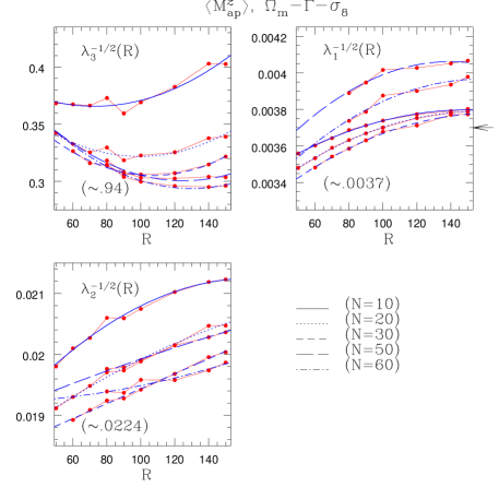
Figure 3: The variance $\sigma_{i}=\lambda_{i}^{-1/2}$ of the three eigenvectors of the Fisher matrix ${\bf F}$, corresponding to ($\Omega_{\rm m}$, $\Gamma$, $\sigma_{8}$) and a flat Universe, for $\langle M_{\rm ap}^{2}\rangle$. Various surveys $(N,R)$ (Sect. 3.1) are compared. The results for the $300\cdot 13^{\prime\,2}$ survey is written in brackets in each panel and, while within the range of the plot, marked with an arrow. The smooth curves are second-order polynomial fits to the data points.

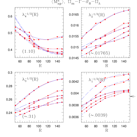
Figure 4: The variance $\sigma_{i}=\lambda_{i}^{-1/2}$ of the four eigenvectors of the Fisher matrix ${\bf F}$, corresponding to ($\Omega_{\rm m}$, $\Gamma$, $\sigma_{8},\Omega_{\Lambda}$), for $\langle M_{\rm ap}^{2}\rangle$. See Fig. 3 for more details.

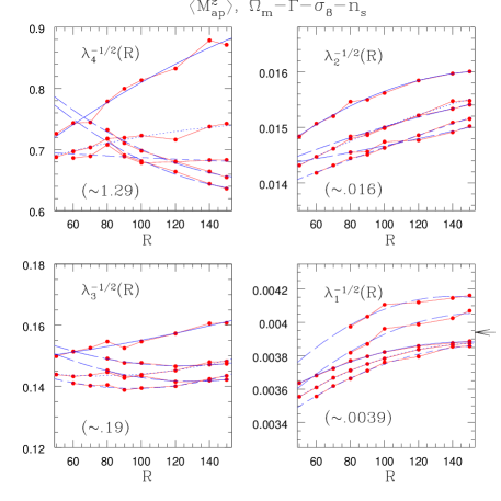
Figure 5: The variance $\sigma_{i}=\lambda_{i}^{-1/2}$ of the four eigenvectors of the Fisher matrix ${\bf F}$, corresponding to ($\Omega_{\rm m}$, $\Gamma$, $\sigma_{8},n_{\rm s}$) and a flat Universe, for $\langle M_{\rm ap}^{2}\rangle$. See Fig. 3 for more details.

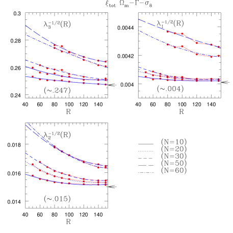
Figure 6: The variance $\sigma_{i}=\lambda_{i}^{-1/2}$ of the three eigenvectors of the Fisher matrix ${\bf F}$, corresponding to ($\Omega_{\rm m}$, $\Gamma$, $\sigma_{8}$) and a flat Universe, for $\xi_{\rm tot}$. See Fig. 3 for more details.

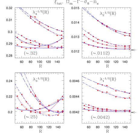
Figure 7: The variance $\sigma_{i}=\lambda_{i}^{-1/2}$ of the four eigenvectors of the Fisher matrix ${\bf F}$, corresponding to ($\Omega_{\rm m}$, $\Gamma$, $\sigma_{8},n_{\rm s}$) and a flat Universe, for $\xi_{\rm tot}$. See Fig. 3 for more details.

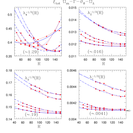
Figure 8: The variance $\sigma_{i}=\lambda_{i}^{-1/2}$ of the four eigenvectors of the Fisher matrix ${\bf F}$, corresponding to ($\Omega_{\rm m}$, $\Gamma$, $\sigma_{8},\Omega_{\Lambda}$), for $\xi_{\rm tot}$. See Fig. 3 for more details.

In Figs. 3–8 we show the variance $\sigma_{i}=1/\lambda_{i}^{-1/2}$ corresponding to the $i^{\rm th}$ eigenvector of the Fisher matrix. The cosmological parameter combinations are the same than in the previous section. We comment on the dependence on the patch radius $R$ and number of lines of sight per patch $N$ in the following sections.

3.4.1 Aperture mass dispersion

In the majority of the cases, the variance $\sigma_{n}$ of the dominating, worst constrained parameter combination shows a minimum for some $R_{0}$ within the probed range of patch radii. This confirms the result of KS04, where the MVB (which is dominated by $\sigma_{n}$) also showed a minimum. The optimal radius $R_{0}$ decreases towards smaller $N$, thus, compact configurations yield better results than sparse patches. This is also reflected in the fact that patches with high $N$ are preferred over those with small $N$. For the other, less dominant eigenvectors, the corresponding variance is (in most cases) a monotonic increasing function of $R$. All this implies that in order to obtain constraints on parameter combinations, compact, densely sampled patches will give the best results.

3.4.2 Two-point correlation function

The radius $R_{0}$ where the variance $\sigma_{n}$ of the dominant eigenvector takes a minimum is reached for larger $R$ than for $\langle M_{\rm ap}^{2}\rangle$. In some cases, $R_{0}$ exceeds 150 arc minutes, which is the maximum of the probed range of radii. In most of the time, the variances $\sigma_{i}$ are decreasing functions of $R$ in contrast to the aperture mass dispersion. These results show that a small cosmic variance is more important for $\xi_{\rm tot}$ than a rigorous sampling of intermediate scales. Strategies with sparse patches probing a large number of independent regions on the sky and, at the same time, capturing shear information on large angular scales will provide the best constraints on cosmological parameters.

We compare the individual contributions of $\xi_{+}$ and $\xi_{-}$ to the variances $\sigma_{i}$ of the joint estimator $\xi_{\rm tot}$. The latter is dominated by $\xi_{+}$ and the dependence on the survey strategy is very similar for both. The contribution from $\xi_{-}$, however, resembles the one corresponding to the aperture mass dispersion, since both statistics sample the convergence power spectrum in a similar way. In particular, $\xi_{-}$ and $\langle M_{\rm ap}^{2}\rangle$ do not probe large scales in contrast to $\xi_{+}$ (see eq. 1). The corresponding filter functions for the former two statistics, ${\rm J}_{4}(\eta)$ and $[{\rm J}_{4}(\eta)/\eta^{2}]^{2}$, respectively, are both proportional to $\eta^{4}$ for small $\eta$, suppressing large scales. On the contrary, for the latter statistics, ${\rm J}_{0}$ is constant for small arguments. A survey which covers large angular scales at the expense of a dense sampling of small and medium scales will therefore not be optimal for $\xi_{-}$ and $\langle M_{\rm ap}^{2}\rangle$, but efficient for $\xi_{+}$.

3.4.3 Comparison with the uncorrelated lines-of-sight-survey

The $300\cdot 13^{\prime\,2}$-survey of uncorrelated lines of sight shows larger values for $\sigma_{i},\,i=2\ldots n$ than the patch surveys, corresponding to poorer constraints on cosmological parameters. However, the smallest variance $\sigma_{1}$ is reached asymptotically for patch strategies with large $R$ and $N=10,20,30$. These surveys consisting of a large number of sparse patches corresponding to a small cosmic variance are those which are most similar to the uncorrelated lines-of-sight-survey. Since for the 2PCF a small cosmic variance is crucial, the patch strategies show not much improvement in $\sigma_{1}$ over the $300\cdot 13^{\prime\,2}$-survey (unless both $\Omega_{\rm m}$ and $\Omega_{\Lambda}$ are free parameters, see Fig. 8). This is in contrast to the aperture mass statistics, where the improvement in $\sigma_{1}$ is more than a factor of two.

With decreasing $i$, the variance $\sigma_{i}$ of the eigenvector $\@vec{p}_{i}$ becomes less sensitive on the survey geometry. The measurement of the best constrained combinations of parameters can therefore not efficiently be improved and even the $300\cdot 13^{\prime\,2}$-survey will yield good results.

The $300\cdot 13^{\prime\,2}$-survey can compete with a patch strategy regarding the best constrained eigenvectors which contribute least to the parameter uncertainties. For the dominant parameter combinations, the patch strategies are superior and yield much better constraints on cosmological parameters.

3.5 Inclusion of additional parameters

To include more cosmological parameters in our analysis, we consider a survey of 141 square degree area. This corresponds to an enlargement of the $(30,100^{\prime})$ strategy, consisting of 100 instead of 10 independent patches. The eigenvectors and corresponding eigenvalues are shown in Table 7.

The first, best determined eigenvector is orthogonal to the $\Omega_{\rm m}$-$\sigma_{8}$ degeneracy direction, as in Sect. 3.3. The second best direction is orthogonal to the prominent $\Gamma$-$n_{\rm s}$ degeneracy direction, but with a strong contribution from $\Omega_{\rm m}$. The worst constrained eigenvector $\@vec{p}_{7}$ is almost solely dependent on the redshift parameters $z_{0}$ and $\beta$.

Table 7: Eigenvectors of the Fisher matrix for all 7 parameters from a 141 square degree survey.

	$\@vec{p}_{1}$	$\@vec{p}_{2}$	$\@vec{p}_{3}$	$\@vec{p}_{4}$	$\@vec{p}_{5}$	$\@vec{p}_{6}$	$\@vec{p}_{7}$	$\triangle\Theta_{i}$
$\Omega_{\rm m}$	$\phantom{-}0.639$	$-0.563$	$-0.016$	$\phantom{-}0.260$	$\phantom{-}0.002$	$-0.454$	$\phantom{-}0.014$	$0.622$
$\Gamma$	$\phantom{-}0.392$	$\phantom{-}0.691$	$-0.404$	$\phantom{-}0.219$	$-0.360$	$-0.168$	$\phantom{-}0.002$	$0.233$
$\sigma_{8}$	$\phantom{-}0.503$	$-0.049$	$-0.359$	$-0.556$	$\phantom{-}0.301$	$\phantom{-}0.463$	$-0.034$	$0.669$
$z_{0}$	$\phantom{-}0.311$	$\phantom{-}0.088$	$\phantom{-}0.580$	$-0.074$	$-0.317$	$\phantom{-}0.283$	$\phantom{-}0.611$	$4.099$
$n_{\rm s}$	$\phantom{-}0.176$	$\phantom{-}0.335$	$\phantom{-}0.266$	$\phantom{-}0.437$	$\phantom{-}0.767$	$\phantom{-}0.078$	$\phantom{-}0.025$	$0.218$
$\beta$	$-0.236$	$-0.071$	$-0.469$	$\phantom{-}0.011$	$\phantom{-}0.236$	$-0.196$	$\phantom{-}0.791$	$5.292$
$\Omega_{\Lambda}$	$-0.038$	$-0.279$	$-0.285$	$\phantom{-}0.615$	$-0.188$	$\phantom{-}0.653$	$\phantom{-}0.004$	$0.885$
$\sigma_{i}$	$\phantom{-}0.001$	$\phantom{-}0.004$	$\phantom{-}0.033$	$\phantom{-}0.063$	$\phantom{-}0.117$	$\phantom{-}1.354$	$\phantom{-}6.685$

3.6 Local degeneracy directions

From the Fisher matrix, we quantify the local direction of degeneracy between the parameter pairs $(\Omega_{\rm m},\sigma_{8})$ and $(\Gamma,n_{\rm s})$. For each pair, we marginalise over the remaining parameters out of $(\Omega_{\rm m},\sigma_{8},\Gamma$, $n_{\rm s})$ for a flat Universe, and find

$$\sigma_{8}\,\Omega_{\rm m}^{0.48}=0.56\quad\mbox{and}\quad n_{\rm s}\,\Gamma^{0.3}=0.6,$$ (9)

assuming a power-law dependence between parameter pairs which is usually found in likelihood analysis. These numerical coefficients are basically the same for $\xi_{\rm tot}$ and $\langle M_{\rm ap}^{2}\rangle$. The resulting degeneracy directions are in agreement with Kilbinger & Schneider (2005), even though a non-Gaussian shear field was used to calculate the covariance in this previous work. Marginalisation over the hidden parameters increases the volume of the error ellipsoid and also alters the orientation of its axes in parameter space. However, the general degeneracy direction is similar for various marginalised parameters, see Figs. 9 and 10. We conclude that the directions of near-degeneracy between the considered parameter pairs are robust against the inclusion of non-Gaussianity of the shear field, but less stable against the addition of cosmological parameters. In Fig. 9 we show the 1$\sigma$-ellipses for the parameter pair ($\Omega_{\rm m}$, $\Gamma$) using all four estimators $\xi_{+}$, $\xi_{-}$, $\xi_{\rm tot}$ and $\langle M_{\rm ap}^{2}\rangle$. Slight misalignments in the degeneracy directions from $\xi_{+}$ compared with $\xi_{-}$ leads to improved constraints from the combined estimator $\xi_{\rm tot}$.

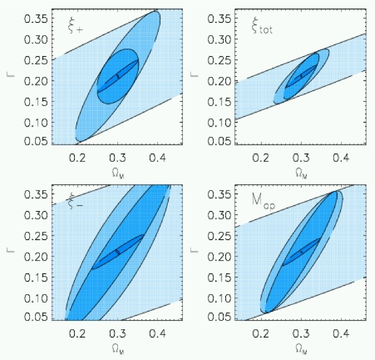
Figure 9: 1$\sigma$ error ellipses in the $\Omega_{\rm m}$-$\Gamma$ plane. From small to large ellipses, successive marginalisation over $\sigma_{8},n_{\rm s},\Omega_{\Lambda},\beta,z_{0}$ (except the ones that are plotted) was performed. The four panels correspond to the four estimators $\xi_{+}$, $\xi_{-}$, $\xi_{\rm tot}$ and $\langle M_{\rm ap}^{2}\rangle$ as indicated.

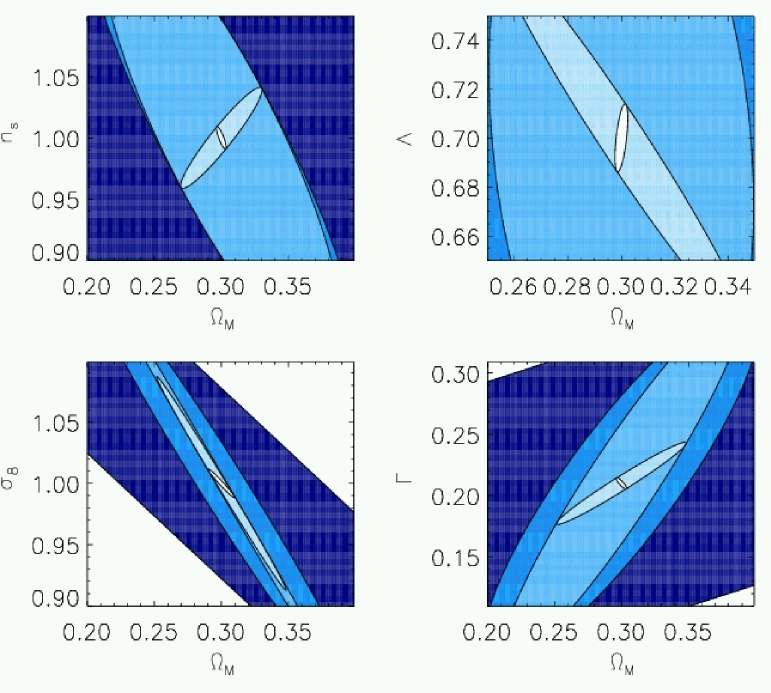
Figure 10: 1$\sigma$ error ellipses for $\Omega_{\rm m}$ and $\sigma_{8}$, $n_{\rm s}$, $\Omega_{\Lambda}$ and $\Gamma$, respectively, in the four panels. From small to large ellipses, successive marginalisation over the remaining parameters out of $(\Gamma,\sigma_{8},n_{\rm s},\Omega_{\Lambda},\beta,z_{0})$ was performed. The estimator is $\langle M_{\rm ap}^{2}\rangle$ and the survey strategy the 141 square degree survey.

3.7 Effect of the survey depth on the principal components

For surveys with fixed $N=60$ and varying $R$, we calculate the Fisher matrix for three different source redshift distribution functions, parametrised by $z_{0}=0.8,1.0$ and 1.2, respectively. The variance $\sigma_{i}$ of the principal components of the Fisher matrix corresponding to the three parameters ($\Omega_{\rm m},\sigma_{8}$, $\Gamma$) is shown in Fig. 11. The general characteristics of $\lambda_{i}^{-1/2}$ as a function of $R$ does not change with the survey depth and simply gets scaled. The variance corresponding to the first two eigenvectors decrease with increasing survey depth, corresponding to a smaller error on the parameter measurement. However and unexpectedly, the principal component corresponding to the largest variance $\sigma_{3}$ is best determined for the most shallow survey with $z_{0}=0.8$. This principal component takes little contribution from $\Gamma$ and points in the $\Omega_{\rm m}$-$\sigma_{8}$ degeneracy direction. We repeat the PCA without the shape parameter and found a similar result. Also when marginalising over additional parameters, the largest eigenvalue of the Fisher matrix is smallest for $z_{0}=0.8$.

This unexpected effect is a local one, present in the Fisher matrix only. In order to see the global behaviour, we calculate the likelihood in the $\Omega_{\rm m}$-$\sigma_{8}$ plane and find that the confidence levels get tighter with increasing source redshift. The near-degeneracy is less pronounced if the survey is deeper and more information about the large-scale structure is collected in the shear signal. Moreover, the curvature of confidence levels increases with increasing $z_{0}$ which leads to a larger bending of the curves of constant likelihood. The shear correlation from different source galaxy redshift distributions allows one to constrain slightly different regions in parameter space. This fact is made use of in shear tomography to lift the parameter near-degeneracies (Hu 1999).

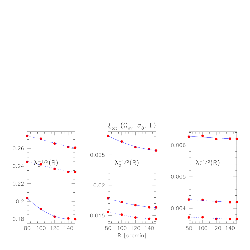
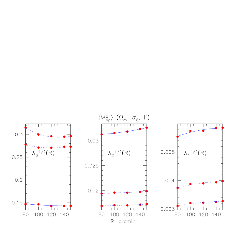
Figure 11: The variance $\sigma_{i}=\lambda_{i}^{-1/2}$ of the three eigenvectors of the Fisher matrix corresponding to $(\Omega_{\rm m},\sigma_{8},\Gamma)$ and a flat Universe, using the 2PCF (top) and the aperture mass dispersion (lower panels). The curves show different survey depth where solid, dashed and dotted lines correspond to $z_{0}=0.8,1.0$ and 1.2, respectively.

3.8 Effect of the source galaxy density on the principal components

For the same survey types ($N=60$) and the parameters $\Omega_{\rm m},\sigma_{8}$ and $\Gamma$ as in the previous section, we compute the Fisher matrix for three different surface densities of background galaxies, $n_{\rm gal}=20,30$ and 40 per square arc minute. The variance $\sigma_{i}$ of the three principal components of the Fisher matrix is plotted as a function of patch radius $R$ in Fig. 12, corresponding to measurements of the 2PCF and the aperture mass dispersion, respectively. As expected, $\sigma_{i}$ decreases with increasing $n_{\rm gal}$ since more background galaxies provide a better sampling of the shear field. The minimum variance for $\sigma_{3}$ at $R_{0}\approx 130$ in the case of $\langle M_{\rm ap}^{2}\rangle$ does not change with noise level.

In this work, we treated the survey depth, parametrised by $z_{0}$, and the number density of background galaxies $n_{\rm gal}$ as independent survey characteristics. For a realistic survey however, this assumption is not justified in general since an increase in depth implies a higher galaxy number density.

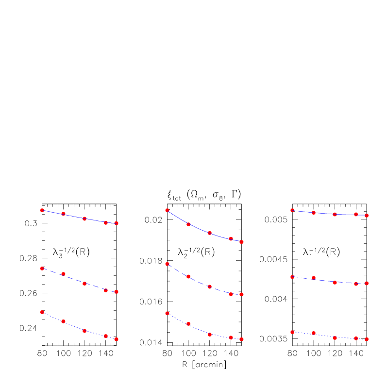
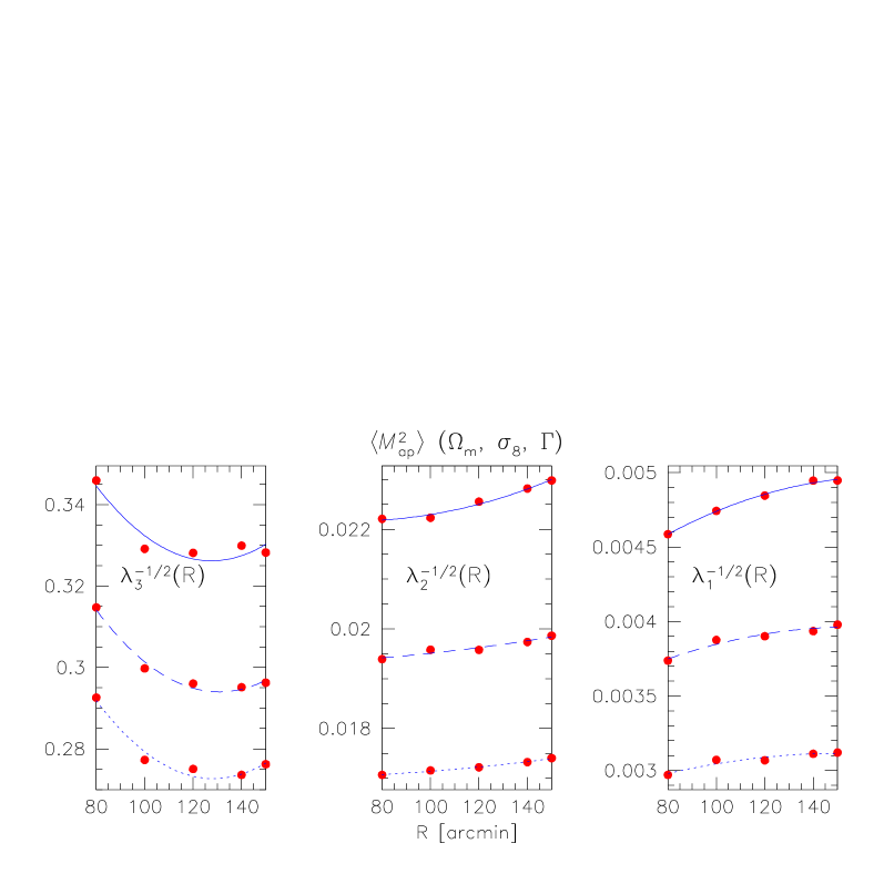
Figure 12: The variance $\sigma_{i}=\lambda_{i}^{-1/2}$ of the three eigenvectors for the Fisher matrix corresponding to $(\Omega_{\rm m},\sigma_{8},\Gamma)$ and a flat Universe, using the 2PCF (top) and the aperture mass dispersion (lower panels). The curves show different survey depth where solid, dashed and dotted lines correspond to $n_{\rm gal}=20,30$ and 40 per square arc minute, respectively.

3.9 Principal components and the error ellipsoid volume

We investigate the geometric mean $\rho=(\lambda_{1}\dots\lambda_{n})^{1/n}$ of the $n$ eigenvalues of the Fisher matrix ${\bf F}$. The equivalent radius of the Fisher error ellipsoid, which is the radius of an $n$-sphere with the same volume, is $\rho^{-1/2}=(\det{{\bf F}})^{-1/2n}$.

In Figs. 13 and 14 we plot the effective error ellipse radius $\rho^{-1/2}$ as a function of $R$ for survey geometries $(N,R)$ using different parameter combinations and estimators. Since $\rho^{-1/2}$ is dominated by the largest variance $\sigma_{n}$ (smallest eigenvalue of ${\bf F}$), it shows a similar behaviour (see Sect. 3.4). However, the minimum seems to be reached at smaller $R_{0}$ an therefore the optimal survey radius is smaller than the previous sections implied. The $300\cdot 13^{\prime\,2}$-survey (see Fig. 13 and Table 8) yields comparable results than for the patch geometries if $\xi_{+}$ is used. $\xi_{-}$ and $\langle M_{\rm ap}^{2}\rangle$ (not shown), however, strongly suffer from the lack of scales larger than 20 arc minutes which results in a much larger error ellipsoid.

Table 8: The effective radius of the Fisher error ellipse $\rho^{-1/2}$ for the $300\cdot 13^{\prime\,2}$-survey, corresponding to two combinations of cosmological parameters. The values of $\rho^{-1/2}$ for various patch strategies $(N,R)$ are displayed in Fig. 14.

	$(\Omega_{\rm m},\Gamma,\sigma_{8})$	$(\Omega_{\rm m},\Gamma,\sigma_{8},\Omega_{\Lambda})$
$\xi_{\rm tot}$	0.024	0.061
$\xi_{+}$	0.028	0.062
$\xi_{-}$	0.130	0.163

In Fig. 14, the results for the 2PCFs $\xi_{+}$ and $\xi_{-}$ are compared. As already mentioned before, $\xi_{\rm tot}$ is dominated by $\xi_{+}$ and shows a similar behaviour. The shape of the $\xi_{-}$-curves on the other hand resembles the one for $\langle M_{\rm ap}^{2}\rangle$.

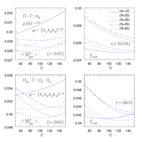
Figure 13: The effective radius $\rho^{-1/2}$ of the Fisher error ellipsoid as a function of survey radius $R$. The left panels correspond to $\langle M_{\rm ap}^{2}\rangle$, the right panel to $\xi_{\rm tot}$. In the upper two panels, the parameter combination is $(\Omega_{\rm m},\Gamma,\sigma_{8})$, in the lower panels it is $(\Omega_{\rm m},\Gamma,\sigma_{8},\Omega_{\Lambda})$. The numbers in parenthesis correspond to $\rho^{-1/2}$ from the $300\cdot 13^{\prime\,2}$-survey. The definition of $\rho$ is given in the panel as a reminder.

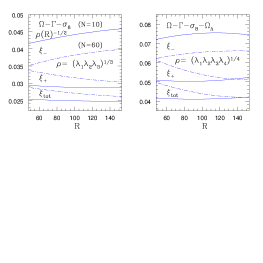
Figure 14: The effective radius $\rho^{-1/2}$ of the Fisher error ellipsoid corresponding to ($\Omega_{\rm m},\Gamma,\sigma_{8})$ (left panel) and $(\Omega_{\rm m},\Gamma,\sigma_{8},\Omega_{\Lambda})$ (right panel). The three estimators $\xi_{-}$, $\xi_{+}$ and $\xi_{\rm tot}$ are compared using for surveys with sparse ($N=10$, solid lines) and dense ($N=60$, dash-dotted lines) geometries.

3.10 Principal components of the scaled Fisher matrix

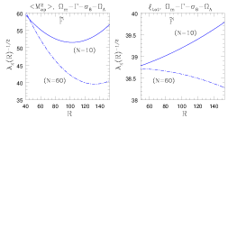
Figure 15: The variance $\sigma_{4}=\lambda_{4}^{-1/2}$ of the dominant eigenvalue of the scaled Fisher matrix $\tilde{F}$ for the parameters ($\Omega_{\rm m},\Gamma,\sigma_{8},\Omega_{\Lambda}$), as a function of the patch radius $R$. Solid lines correspond to surveys with $N=10$, dash-dotted curves are for $N=60$.

The scaled Fisher matrix $\tilde{F}$ is defined as

$$\tilde{F}_{ij}={F_{ij}\over\sqrt{F_{ii}F_{jj}}}.$$ (10)

Its inverse $\tilde{{\bf F}}^{-1}$ represents the covariance of the normalised (unit variance), correlated Gaussian variables $\tilde{\Theta}_{j}$ constructed from the original cosmological parameters, $\tilde{\Theta}_{j}=\Theta_{j}/\sqrt{\langle\Theta_{j}^{2}\rangle}$. The scaled parameters can be compared with each other in a straightforward way, and their correlation gets more underlined. The variation with patch radius $R$ of the eigenvalues of the scaled Fisher matrix matches well with their unscaled counterparts. In Fig. 15 we plot the variance of the dominant eigenvector $\lambda_{n}^{-1/2}(R)$ for geometries with $N=10$ and $N=60$, respectively, and the cosmological parameters $(\Omega_{\rm m},\Gamma,\sigma_{8},\Omega_{\Lambda})$.

3.11 Principal components and the use of priors

Additional priors on parameters modify the original Fisher matrix $F$ to $\hat{F}=F+C^{-1}$. For example, a Gaussian prior for the $i^{\rm th}$ parameter with variance $s_{i}$ corresponds to $C_{ij}^{-1}=\delta_{ij}\,s_{i}^{-2}$. Priors lower the eigenvalues. Since the reduction is the larger the smaller the eigenvalue is, the dominant eigenvector with the smallest eigenvalue is affected most by priors. The effect of a prior on the variance of this eigenvector is shown in the upper right panel of Fig. 1 and in Fig. 16. In Fig. 1, the priors $s(p_{i})$ are 0.003 for $\Omega_{\rm m},\sigma_{8}$ and $\Gamma$, 0.03 for $\Omega_{\Lambda}$, 0.1 for $n_{\rm s}$ and $z_{0}$ and 1 for $\beta_{p}$. For the three curves, priors are added for parameters as indicated in the panel. The more priors are included, the more is the large, dominant variance affected, and the curve $\sigma_{i}$ as a function of $i$ becomes less steep.

The addition of a prior also flattens the curve $\sigma_{n}(R)$ as a function of patch radius $R$ and the difference between the surveys becomes less pronounced, making the optimisation less effective, see Fig. 16. From Fig. 17 one infers that the prior of a flat Universe ($\Omega_{\Lambda}=1-\Omega_{\rm m}$) corresponds to a higher variance $\sigma_{n}$ than a constant $\Omega_{\Lambda}=0.7$ prior.

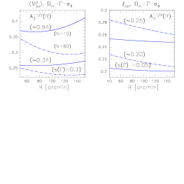
Figure 16: The variance of the dominant eigenvector $\sigma_{3}$ is plotted for patch geometries with $N=10$ (solid lines) and $N=60$ (dash-dotted), for $\langle M_{\rm ap}^{2}\rangle$ (left panel) and $\xi_{\rm tot}$ (right panel). The three cosmological parameters under consideration are $\Omega_{\rm m}$, $\Gamma$ and $\sigma_{8}$. The upper curves correspond to the case without prior. For the lower pair of curves, and additional prior on $\Gamma$ of $s(\Gamma)=0.3\,(0.05)$ is assumed for $\langle M_{\rm ap}^{2}\rangle\;(\xi_{\rm tot})$, respectively. The values in the parenthesis denote $\sigma_{n}$ the $300\cdot 13^{\prime\,2}$-survey.

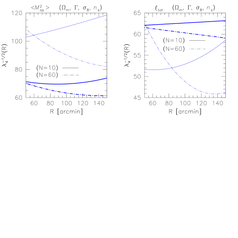
Figure 17: The variance of the dominant eigenvector $\sigma_{4}=\lambda_{4}^{-1/2}$ of the scaled Fisher matrix $\tilde{F}$ for the parameters $(\Omega_{\rm m},\Gamma,\sigma_{8},n_{\rm s}$), as a function of the patch radius $R$. Thick curves are for a flat Universe, thin curves for constant $\Omega_{\Lambda}$. Solid lines correspond to $N=10$, dash-dotted lines to $N=60$.

4 Summary and discussion

We study the design of cosmic shear survey with the means of a principal component analysis of the Fisher information matrix. Although only a local approximation of the likelihood, the Fisher matrix provides a simple and cost-effective method to predict cosmological parameter constraints and to investigate degeneracies between parameters. We compare realistic survey designs with non-trivial topology. In most of the previous analyses (an exception being KS04) either simple monolithic survey topologies were assumed or the correlation of power for different Fourier modes was neglected. In this work, we use the full covariance matrix of second-order shear statistics corresponding to a complicated, non-trivial distribution of lines of sight. We assume the shear field to be Gaussian which leads to an underestimation of the covariance on intermediate angular scales between $\sim$ 1 and 10 arc minutes.

The eigenvectors or principal components of the Fisher matrix determine linear, orthogonal combinations of cosmological parameters. We find that these vectors are only little affected by the survey characteristics. The same is true for the directions of near-degeneracy between parameters. However, the eigenvalues change significantly with survey geometry. The eigenvector of the Fisher matrix which dominates the errors of the cosmological parameters has the smallest eigenvalue corresponding to the largest variance. To maximise this eigenvalue, which is to minimise the error on this eigenvector, the shear correlation on large angular scales up to several degree has to be measured. The dependence on the sampling of shear correlation is different for the correlation function $\xi_{\rm tot}$ and the aperture mass dispersion $\langle M_{\rm ap}^{2}\rangle$. For $\xi_{\rm tot}$, a survey consisting of sparse patches with a small cosmic variance yields the smallest errors. Using $\langle M_{\rm ap}^{2}\rangle$, dense and slightly smaller patches are preferred.

We consider various combinations of the cosmological parameters $\Omega_{\rm m},\Gamma,\sigma_{8},n_{\rm s},\Omega_{\Lambda}$ and the source galaxy redshift characteristics $z_{0}$ and $\beta$ (see Sect. 2.1). If not more than three parameters are to be determined from our survey (the other parameters being fixed), the dominant eigenvector of the Fisher matrix comprises more than 99 % of the parameter errors. For more than three free parameters, the first two principal components are responsible for most of the parameter errors.

Changing the number density of source galaxies, the depth of the survey, the intrinsic ellipticity dispersion or the total survey area simply causes a scaling of the eigenvalues. The optimal survey setting is not affected by changes in those parameters. Furthermore, introducing external priors on some parameters does not result in a different optimal setting. However, this optimum becomes less pronounced so that optimisation of the survey design will be less important. If a flat Universe is taken as a prior, the dependence on the survey geometry is much weaker than for the prior $\Omega_{\Lambda}={\rm const}$.

The dominant principal component shows an unexpected behaviour when the survey depth $z_{0}$ is varied. The error on the corresponding parameter combination increases for increasing $z_{0}$ in the range of $z_{0}=0.8\ldots 1.2$. However, this effect is only local and disappears when considering the likelihood function, which shows strong non-Gaussian features not present in the Fisher matrix.

As survey sizes increase it will be desirable to estimate an increasing number of parameters independently from weak lensing surveys alone such as the equation of state of dark energy or its variation with redshift (Hu 1999; Heavens 2003). However, parameter near-degeneracies inherent in weak lensing observables make additional data from different cosmology experiments very valuable in breaking such degeneracies. On the other hand, priors from CMB or SN observations can be used in the future to optimise the design of smaller surveys by using principal components of the joint Fisher matrix (e.g. Crittenden & Pogosian 2005 provide results of joint PCA of different data sets in a similar context).

We conclude that existing tools such as generalised eigenmode analyses (Karhunen 1947; Loève 1948; Vogeley & Szalay 1996; Matsubara et al. 2000; Kilbinger & Munshi 2005) and principal component analyses which we have studied here will be very useful in optimising future weak lensing surveys.

References

- (1) Bacon, D.J., Réfrégier, A., & Ellis, R. 2000, MNRAS 318, 625
- (2) Bacon, D.J., Réfrégier, A., Clowe, D., & Ellis R. 2001, MNRAS 325, 1065
- (3) Bacon, D.J., Massey R., Réfrégier, A., & Ellis R. 2003, MNRAS 344, 673
- (4) Bartelmann, M., & Schneider, P. 2001, Phys. Rep. 340, 291
- (5) Brainerd, T.G., Blandford, R.D, & Smail, I. 1996, ApJ, 466, 623
- (6) Brown, M., Taylor, A.N., & Bacon, D.J., et al. 2003, MNRAS 341, 100
- (7) Colless, M., Dalton, G., Maddox, S., et al. 2001, MNRAS, 328, 1039
- (8) Contaldi, C., Hoekstra H., & Lewis, A. 2003, PRL, 90, 1303
- (9) Crittenden R.G., & Pogosian L. 2005, astro-ph/0510293
- (10) Efstathiou, G. 2002, MNRAS, 332, 193
- (11) Efstathiou, G., & Bond, J.R. 1999, MNRAS, 304,75
- (12) Groch, H., Dell’Antonio, I., Dey, A., Jannuzi, B.T., et al. 2000, Bulletin of the AAS, 32, 1577
- (13) Hamana, T., Miyazaki, S., Shimasaku, et al. 2003, ApJ, 597, 98
- (14) Hamilton, A.J.S. 1997, MNRAS, 289, 295
- (15) Hamilton, A.J.S., & Tegmark M. 2000, MNRAS, 312, 285
- (16) Hämmerle, H., Miralles, J.M., Schneider, P., Erben, T., & Fosbury, R.A. 2002, A&A, 385, 743
- (17) Heavens, A. 2003, MNRAS, 343, 1327
- (18) Hoekstra, H., Mellier, Y., van Waerbeke, L., et al. 2005, submitted to ApJ, also astro-ph/0511089
- (19) Hoekstra, H., Yee, H.K.C., & Gladders, M. 2002a, ApJ, 577, 595
- (20) Hoekstra, H., Yee, H.K.C., Gladders, M., et al. 2002b, ApJ, 572, 55
- (21) Hu, W. 1999, ApJ, 522, L21
- (22) Hu, W., & Keeton, C.R. 2002, Phys. Rev. D, 66, 3506
- (23) Hu, W., & Tegmark, M. 1999, ApJ, L65
- (24) Huterer, D., & Cooray, A. 2005, Phys. Rev. D, 71, 023506
- (25) Huterer, D., & Starkman, G. 2003, PRL, 90, 031301
- (26) Ishak, M., Hirata, C.M., McDonald, P., & Seljak, U. 2004, Phys. Rev. D, 69, 083514
- (27) Jarvis, M., Bernstein, G.M., Fisher, P., et al. 2002, ApJ, 125, 1014
- (28) Jarvis, M., & Jain, B. 2004, submitted to ApJ, also astro-ph/0412234
- (29) Kaiser, N. 1992, ApJ, 388, 272
- (30) Kaiser, N. 1998, ApJ, 498, 26
- (31) Kaiser, N. 2000, ApJ, 537, 555
- (32) Karhunen, H. 1947, Ann. Acad. Science Finn. Ser. A. I., 37
- (33) Kilbinger, M., & Munshi, D. 2005, MNRAS in press, also astro-ph/0509548
- (34) Kilbinger, M., & Schneider, P. 2004, A&A, 413, 465 (KS04)
- (35) Kilbinger, M., & Schneider, P. 2005, A&A, 442, 69
- (36) Loève, M. 1948, Processes Stochastiques et Mouvement Brownien, (Hermann, Paris France)
- (37) Maoli, R., van Waerbeke, L., Mellier, Y., et al. 2001, A&A, 368, 766
- (38) Massey, R., Rhodes, J., Réfrégier, A., et al. 2004, AJ, 127, 3089
- (39) Mastsubara, T., Szalay, A.S., & Landy, S.D. 2000 ApJ, 535, L1
- (40) Mellier, Y. 1999, ARA&A, 37, 127
- (41) Peacock, J.A., & Dodds, S.J. 1996, MNRAS, 280, L19
- (42) Rocha, G., Trotta, R., Martins, C.J.A.P., et al. 2004, MNRAS, 352, 20
- (43) Réfrégier, A. 2003, ARA&A, 41, 645R
- (44) Réfrégier, A., Rhodes, J., & Groth, E.J. 2002, ApJ, 572L,131
- (45) Rhodes, J., Réfrégier, A., & Groth, E.J. 2001, ApJ, 552L, 85
- (46) Seljak, U., McDonald, P., & Makarov, A. 2003, MNRAS, 342, L79
- (47) Schneider, P. 1996, MNRAS, 283, 837
- (48) Schneider, P. 2005, in Kochanek, C.S., Schneider, P., Wambsganss, J.: Gravitational Lensing: Strong, Weak & Micro. Lecture Notes of the 33rd Saas-Fee Advanced Course, G. Meylan, P. Jetzer and P. North (eds.), Springer-Verlag: Berlin, also astro-ph/0509252
- (49) Schneider, P., van Waerbeke, L., Jain, B., & Kruse, G. 1998, MNRAS, 296, 873
- (50) Schneider, P., van Waerbeke, L., Kilbinger, M. & Mellier, Y. 2002a, A&A, 396, 1
- (51) Schneider, P., van Waerbeke, L., & Mellier, Y. 2002b, A&A, 389, 729
- (52) Semboloni, E., Mellier, Y., van Waerbeke, L., Hoekstra, H., et al. 2005, submitted to A&A, also astro-ph/0511090
- (53) Spergel, D.N., Verde, L., Peiris, H.V., et al. 2003, ApJS, 148, 175
- (54) Tegmark, M., Taylor, A., & Heavens, A. 1997, Ap.J., 480, 22
- (55) Tegmark, M., Hamilton, A.J.S., Strauss, M.A., Vogeley, M.S., Szalay, A.S. 1998, ApJ, 499, 555
- (56) Tereno, I, Dore, O., van Waerbeke, L., & Mellier, Y. 2005, A&A, 429, 383
- (57) Tyson, J.A., Wittman, D., Hennawi, J.F., & Spergel, D.N. 2002a, Proc. 5th Int. UCLA Symp. Sources Detect. Dark Matter, Marina del Rey, ed. D. Cline. Also astro-ph/0209632
- (58) van Waerbeke, L., Mellier, Y., Erben, T., et al. 2000, A&A, 358, 30
- (59) van Waerbeke, L., Mellier, Y., & Hoekstra, H. 2005, A&A, 429, 75
- (60) van Waerbeke, L., Mellier, Y., Pelló, et al. 2002, A&A, 393, 369
- (61) van Waerbeke, L., Mellier, Y., Radovich, M., et al. 2001, A&A, 374, 757
- (62) van Waerbeke, L. & Mellier, Y. 2003, Lecture given at the Aussois winter school, also astro-ph/0305089
- (63) Vogeley, M.S., & Szalay, A.S. 1996, ApJ, 465, 34
- (64) Wang, Y., & Tegmark, M. 2005, Phys. Rev. D, 71, 103513
- (65) Wittman, D.M., Tyson, J., Kirkman, D., Dell’Antonio, I., & Bernstein, G. 2000, Nature, 405, 143
- (66) Wittman, D.M., Tyson, J.A., Dell’Antonio, I.P., et al. 2002, Proc. SPIE, 4836 v.2., also astro-ph/0210118
- (67) York, D.G., Adelman, J., & Anderson, J.E., et al. 2000, AJ, 120, 1579