What can be learned from the lensed cosmic microwave background $B$-mode polarization power spectrum?

Abstract

The effect of weak gravitational lensing on the cosmic microwave background (CMB) temperature anisotropies and polarization will provide access to cosmological information that cannot be obtained from the primary anisotropies alone. We compare the information content of the lensed $B$-mode polarization power spectrum, properly accounting for the non-Gaussian correlations between the power on different scales, with that of the unlensed CMB fields and the lensing potential. The latter represent the products of an (idealised) optimal analysis that exploits the lens-induced non-Gaussianity to reconstruct the fields. Compressing the non-Gaussian lensed CMB into power spectra is wasteful and leaves a tight degeneracy between the equation of state of dark energy and neutrino mass that is much stronger than in the more optimal analysis. Despite this, a power spectrum analysis will be a useful first step in analysing future $B$-mode polarization data. For this reason, we also consider how to extract accurate parameter constraints from the lensed $B$-mode power spectrum. We show with simulations that for cosmic-variance-limited measurements of the lensed $B$-mode power, including the non-Gaussian correlations in existing likelihood approximations gives biased parameter results. We develop a more refined likelihood approximation that performs significantly better. This new approximation should also be of more general interest in the wider context of parameter estimation from Gaussian CMB data.

I Introduction

The goal of many current and forthcoming cosmic microwave background (CMB) experiments is to measure the polarization of the CMB with increasing accuracy (e.g. QUaD Church et al. (2003), BICEP Keating et al. (2003), EBEX Oxley et al. (2004), QUIET and Clover Taylor et al. (2004)). There are several motivations for this: polarization measurements are an important test of the consistency of the cosmological model, as well containing new information, and can break parameter degeneracies which are present if only the CMB temperature power spectrum is analysed Zaldarriaga et al. (1997). A key motivation is the fact that the curl-like $B$-mode polarization is not generated directly from scalar perturbations at last scattering, and thus can potentially reveal the presence of a primordial gravitational wave background, if it exists at a high enough level Kamionkowski et al. (1997); Seljak and Zaldarriaga (1997). A detection of primordial large-angle $B$-mode polarization would thus provide a measure of the expansion rate and hence energy scale of inflation. Apart from the reionization bump around $\ell\simeq 5$, which depends on the optical depth to last scattering, the gravitational wave signal peaks at multipoles $\ell\sim 100$, corresponding to the angle subtended by the horizon size at last scattering, and so large area surveys (a few hundred deg²) will be required to detect it. On smaller scales, the dominant contribution to $B$-mode polarization is expected to be the weak lensing of $E$-modes by large scale structure along the line of sight Zaldarriaga and Seljak (1998).

The lensing signal is sensitive to the gravitational potential, and hence the clustering of matter, mostly at redshifts $\lesssim 10$ Seljak (1996). (At the peak of the lensing deflection power spectrum at multipoles $\ell\sim 40$, more than 95% of the power arises from $z<10$.) Lensing is therefore sensitive to parameters that have little direct effect on the pattern of primordial fluctuations, but affect the late-time growth of large-scale structure. The lensing signal can thus provide us with information which would otherwise be absent from the CMB Metcalf and Silk (1997); Stompor and Efstathiou (1999), such as the properties of dark energy and sub-eV neutrino masses Hu (2002). However, the lensed $B$-modes are significantly non-Gaussian, and this has been shown to degrade markedly the amount of information present in the $B$-mode power spectrum Smith et al. (2004). The non-Gaussianity introduced by weak lensing is also present to a much lesser extent in the CMB temperature anisotropies and $E$-mode polarization signal. It has recently been shown that neglecting this non-Gaussianity does not significantly bias parameter constraints from Planck-quality data, although the effect of weak lensing on the power spectra cannot be neglected Lewis (2005).

In the present paper we consider more fully the question of what parameter information is contained in the lensed $B$-mode power spectrum and how to analyse future spectral data reliably. We concentrate on the $B$-mode spectrum here for the following reason. The expectation is that for future experiments with sufficient signal-to-noise to image the lens-induced $B$-modes, most of the additional parameter information from the lensing effect on the CMB power spectra will come from the $B$-modes. Although the information content of the $B$-mode power spectrum is relatively more affected by the non-Gaussianity than the temperature ($T$) and $E$-mode polarization, that latter must contend with the cosmic variance of the dominant primary (unlensed) contributions. It is well known that for Gaussian fields the observed power spectrum is a sufficient statistic for parameter estimation under ideal survey conditions, but that this is not the case for non-Gaussian fields such as the lensed CMB. Compressing the lensed CMB fields to their power spectra is wasteful leading to a loss of cosmological information. A more optimal analysis would be to use the non-Gaussianity to reconstruct an estimate of the lensing deflection field and the unlensed CMB fields Hu (2001); Hu and Okamoto (2002), or to work directly from the correct non-Gaussian likelihood function Hirata and Seljak (2003a); Hirata and Seljak (2003b). While such analyses are a worthy goal to strive for, they will likely be difficult to implement in practice in the presence of real-world complications such as inhomogeneous noise, complex survey geometries and foreground residuals. A simpler, and probably more robust method to deal with near-future lensed data is to work directly with the lensed fields in a conventional power spectrum analysis.

This paper is organised as follows. In Section II we review how $B$-mode polarization is generated by the weak lensing of $E$-modes, and consider the cosmological parameters which can be constrained using this information, and the degeneracies between them. In Section III we estimate these parameters from simulated lensed data under the assumption that the data are Gaussian, in order to show directly that this leads to false conclusions. In order to account for the non-Gaussianity we need to understand the correlation between the measured power on different scales, and we calculate this in Section IV following Ref. Smith et al. (2004). In Section V we incorporate the non-Gaussian covariance in existing likelihoods used for the analysis of (Gaussian) CMB data but show that this too leads to biased results in simulations. The reason for this deficiency appears to arise from inaccuracies in the current likelihood approximations when applied to data with few degrees of freedom (which extends to higher multipoles for the lensed $B$-modes than for Gaussian fields). We introduce a more accurate likelihood function in Section VI which we show to perform much better on simulated lensed data. An appendix provides further details of the derivation of this new likelihood.

II Cosmological parameters

The action of lensing on the part of the temperature anisotropy and polarization that is generated at recombination is a simple re-mapping that in the flat-sky approximation can be written as

$$X(\bm{n})=\tilde{X}(\bm{n}+\nabla\phi).$$ (1)

Here $\tilde{X}(\bm{n})$ is the unlensed variable ($T$, or the Stokes parameters $Q$ and $U$), $X(\bm{n})$ the lensed value and $\phi$ the lensing deflection field. On the sphere, we need to take care to interpret correctly the meaning of $\nabla\phi$ Challinor and Chon (2002) and to take into account the position-dependence of the co-ordinate basis for polarization. The root-mean-square lensing deflection angle $\sim 3\,\text{arcmin}$ and so the lensing action on CMB fields well above this scale can be evaluated with the gradient approximation:

$$X(\bm{n})\approx\tilde{X}(\bm{n})+\nabla\tilde{X}\cdot\nabla\phi.$$ (2)

Within this approximation, and in the flat-sky limit, we can express the lensed $B$-mode power spectrum as a convolution of the unlensed $E$-mode power spectrum with the power spectrum of the lensing potential $\phi$ Smith et al. (2004):

$$C_{\ell}^{BB}=\int\frac{\mathrm{d^{2}}\bm{\ell}^{\prime}}{(2\pi)^{2}}C_{\ell^{\prime}}^{\tilde{E}\tilde{E}}C_{|\bm{\ell}-\bm{\ell}^{\prime}|}^{\phi\phi}W^{2}(\bm{\ell},\bm{\ell}^{\prime}),$$ (3)

where function $W$ is given by

$$W(\bm{\ell},\bm{\ell}^{\prime})=\bm{\ell}^{\prime}\bm{\cdot}(\bm{\ell}-\bm{\ell}^{\prime})\sin 2(\phi_{\bm{\ell}}-\phi_{\bm{\ell}^{\prime}}),$$ (4)

with $\bm{\ell}=(\ell\cos\phi_{\bm{\ell}},\ell\sin\phi_{\bm{\ell}})$. This is illustrated in Fig. 1, which shows the unlensed $E$-mode and lensing potential power spectra, together with the resulting lensed $B$-mode power spectrum. The power spectra were calculated using camb which includes corrections for curved sky effects and the breakdown of the gradient approximation Challinor and Lewis (2005).

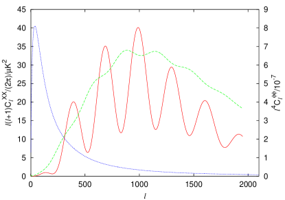
Figure 1: (Colour online) Unlensed $\tilde{E}\tilde{E}$ power spectrum (red solid line) and power spectrum of lensing potential (blue dotted line) which together generate the lensed $BB$ power spectrum (shown by green dashed line, multiplied by a factor of 400).

The lensed $B$-mode power spectrum is thus affected by cosmological parameters which affect either the primary (unlensed) CMB power spectrum $C_{\ell}^{\tilde{E}\tilde{E}}$ or the lensing power $C_{\ell}^{\phi\phi}$. Many of these parameters can be well constrained by the temperature and $E$-mode power spectra, and the lens-induced $B$-modes do not contribute significantly to improving these constraints. Here we concentrate on those parameters that are degenerate with respect to the unlensed CMB spectra. As is well known, the unlensed spectra can provide tight constraints on the physical densities in baryons and cold dark matter, the angular diameter distance to last scattering, the primordial power spectrum, and the optical depth to reionization Efstathiou and Bond (1999). Neutrinos with masses below $\sim 0.3\,\text{eV}$, as implied by current analyses of large-scale structure and the Ly-$\alpha$ forest Seljak et al. (2005), are relativistic at recombination and the only effect of their mass on the unlensed CMB is via the angular diameter distance, $d_{A}$, and a small large-scale contribution to the late integrated Sachs-Wolfe (ISW) effect Eisenstein et al. (1999). Similarly, dark energy parameters, such as the current energy density $\Omega_{\Lambda}h^{2}$, and equation of state $w$ are felt only through $d_{A}$ and the ISW effect. In the inflation-inspired flat models considered here, the parameters $\Omega_{\Lambda}h^{2}$, $w$, and the current density in massive neutrinos $\Omega_{\nu}h^{2}$ (or equivalently the neutrino masses) are highly degenerate with respect to the unlensed CMB, even for cosmic-variance-limited observations. They are collectively constrained only by $d_{A}$, which is now accurately determined to be $13.7\pm 0.5\,\text{Gpc}$ from the CMB alone Spergel et al. (2003). Adding curvature or evolution in the dark-energy sector increases the dimensionality of the degeneracy.

While this ‘geometric’ degeneracy can be easily broken with the inclusion of external data Efstathiou and Bond (1999), it is still worthwhile to consider to what extent the lensing of the CMB helps given its relatively simple and well-understood physics. An early analysis of the temperature and $E$-mode polarization power spectra showed that the weak lensing effect on the power spectra can go some way to breaking the geometric degeneracy Stompor and Efstathiou (1999) since the late-time evolution of the gravitational potential responds differently to variations in the parameters that are geometrically degenerate. Since for multipoles $\ell>100$ the $B$-mode power spectrum is expected to be dominated by weak lensing, this is potentially a much more sensitive probe of the lensing effect than the temperature or $E$-mode power since there is no cosmic variance coming from unlensed $B$-mode polarization. For a given survey, once the sensitivity reaches the limit for imaging the lens-induced $B$-modes (better than $5\,\mu\text{K-arcmin}$) we can expect these to be most constraining. To reach the ultimate cosmic-variance limit considered later in this paper, we require sensitivities around $1\,\mu\text{K-arcmin}$ over a large fraction of the sky. This is similar to the specifications being discussed for a post-Planck orbital experiment dedicated to CMB polarization.

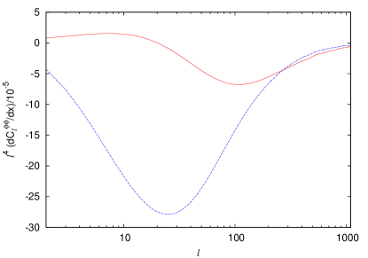
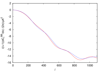
Figure 2: (Colour online) Derivatives of the lensing power spectrum $\ell^{4}C_{\ell}^{\phi\phi}$ (top) and the lensed $B$-mode power spectrum $\ell(\ell+1)C_{\ell}^{BB}/(2\pi)$ (bottom), keeping $\theta_{D}$ fixed (see text). Red solid line: derivatives with respect to $\Omega_{\nu}h^{2}$; blue dashed line: derivatives with respect to $w$ (amplified by a factor of 350 in both plots).

In Fig. 2 we show the derivatives of the lensing potential and $B$-mode power spectra with respect to $w$ and $\Omega_{\nu}h^{2}$ in a flat universe with the physical baryon and cold dark matter densities held fixed at $\Omega_{b}h^{2}=0.024$ and $\Omega_{c}h^{2}=0.111$. The derivatives are taken around $w=-1$ (a cosmological constant) and $\Omega_{\nu}h^{2}=0.004$ with the ratio $\theta_{D}$ of the sound horizon at last scattering to the angular diameter distance held fixed. If we parameterise flat models by $\theta_{D}$, $w$ and $\Omega_{\nu}h^{2}$, both the Hubble parameter $h$ and $\Omega_{\Lambda}h^{2}$ are derived parameters. Our choice of parameterisation is motivated by the geometric degeneracy: the unlensed CMB accurately determines all our parameters expect $w$ and $\Omega_{\nu}h^{2}$ which are themselves very poorly constrained in the absence of external information. The power spectra used to compute these derivatives were computed with the input unlensed power spectra set to zero above the maximum multipole value $\ell_{\text{max}}=2048$ to be consistent with the analyses of simulations presented in the following sections of this paper. We have assumed three families of neutrinos with equal masses. Since $\sum m_{\nu}=\Omega_{\nu}h^{2}\times 94\,\text{eV}$ when all families are non-relativistic, the mass in the fiducial model is $0.13\,\text{eV}$. The total mass is close to the current best limits from cosmological probes Seljak et al. (2005). Given the measurements of (squared) mass differences from atmospheric and solar neutrino experiments, our value of $\Omega_{\nu}h^{2}$ is just at the limit where we can assume mass degeneracy Elgarøy and Lahav (2005). We note also that we have not included any non-linear corrections to the matter power spectrum in computing the spectra in Fig. 2 since the halofit Smith et al. (2003) fitting employed in camb does not currently support massive neutrinos or models with $w\neq-1$. Non-linearities increase the lensing power spectrum beyond $l\sim 300$, and have an effect $>5\%$ on all scales for the $B$-mode spectrum, and a much larger effect on small scales Challinor and Lewis (2005). Non-linearities should thus properly be included in any future data analysis.

The effect of changes in $w$ and $\Omega_{\nu}h^{2}$ on the lensing power spectrum has been discussed in Ref. Kaplinghat et al. (2003). The main effect of changes of $w$ is through the change in the expansion rate. An increase in $w$ at fixed $\theta_{D}$ (or, equivalently, $d_{A}$) requires a reduction in the current dark-energy density and hence $h$. However, increasing $w$ causes dark energy to dominate earlier and the net effect is an initial enhancement of the expansion rate over that for $w=-1$; this causes the gravitational potential to decay earlier and suppresses the lensing effect. Hence the derivative of the lensing potential power spectrum with respect to $w$ is negative; see Fig. 2. The effect on the potential is almost independent of scale, but its time dependence causes a larger fractional change in lensing power on large scales. If we fix the current physical density in dark energy, the effect of massive neutrinos on the gravitational potential vanishes on large scales (larger than the Jeans length of the neutrinos when they first become non-relativistic) since the increased expansion rate is offset by the neutrino clustering. The effect on the lensing power spectrum thus also vanishes at large $\ell$. On scales below the neutrino Jeans length today the neutrinos have never clustered and their mass gives a scale-independent suppression of the gravitational potential similar to the effect of increasing $w$. On intermediate scales, there is a scale-dependent suppression of the lensing power. The additional effect of keeping $\theta_{D}$ fixed is to subtract off a small proportion of the suppression that arises when $\Omega_{\Lambda}h^{2}$ is increased so that neutrino mass then gives a small positive enhancement of lensing power at low $\ell$ and a suppression for larger $\ell$ (Fig. 2). The different scale dependence of the effects of neutrino mass and $w$ allows them to be separated if the lensing potential can be accurately determined. In this way one can determine both $w$ and $\Omega_{\nu}h^{2}$ accurately, whereas neither (nor any combination) can be determined accurately from the unlensed CMB alone. Forecasts for such constraints were given in Ref. Kaplinghat et al. (2003), which used for the errors on $C_{l}^{\phi\phi}$ those expected from an application of the quadratic reconstruction technique of Ref. Hu and Okamoto (2002). This exploits the local scale-scale correlations in the non-Gaussian lensed CMB fields to reconstruct a (noisy) estimate of the deflection field. Improvements in the reconstruction of the deflection field may be possible with more optimal techniques Hirata and Seljak (2003b). Reference Kaplinghat et al. (2003) found that a post-Planck experiment could determine $w$ to within an error of $0.18$ and detect the mass of a single family of massive neutrinos if $m_{\nu}>0.04\,\text{eV}$.

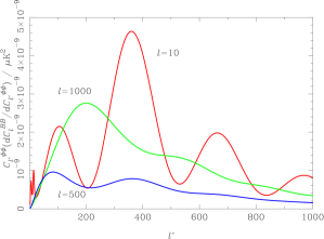
Figure 3: (Colour online) Kernels $C_{\ell^{\prime}}^{\phi\phi}\text{d}C_{\ell}^{BB}/\text{d}C_{\ell^{\prime}}^{\phi\phi}$ for $\ell=10$ (red), $\ell=500$ (blue) and $\ell=1000$ (green). These give (approximately) the contribution to the lensed $B$-mode spectrum from lenses at scale $\ell^{\prime}$.

Figure 2 shows that $w$ and $\Omega_{\nu}h^{2}$ are largely degenerate with respect to their effect on the $B$-mode power spectrum. This is because for no $\ell$ is the dominant contribution to $C_{\ell}^{BB}$ coming from the largest angle lenses for which there is a clear difference between the effects of varying $w$ and $\Omega_{\nu}h^{2}$; for $\ell\gtrsim 200$, the effect of varying $w$ or $\Omega_{\nu}h^{2}$ is almost degenerate in the lensing potential power spectrum and hence in $C_{\ell}^{BB}$. In Fig. 3 we plot the derivatives $C_{\ell^{\prime}}^{\phi\phi}\text{d}C_{\ell}^{BB}/\text{d}C_{\ell^{\prime}}^{\phi\phi}$ as a function of $\ell^{\prime}$ for several values of $\ell$. For any $\ell$, the integral of the kernel over $\ell^{\prime}$ gives the lensed $B$-mode power spectrum at that $\ell$ (in the gradient approximation, Eq. 1). Similarly, for the parameter variations considered here that leave the unlensed $E$-mode power spectrum unchanged, the convolution of the kernel $C_{\ell^{\prime}}^{\phi\phi}\text{d}C_{\ell}^{BB}/\text{d}C_{\ell^{\prime}}^{\phi\phi}$ with the fractional change in $C_{\ell^{\prime}}^{\phi\phi}$ gives the change in the lensed $B$-mode spectrum. The shape of the kernels in Fig. 3 can be understood as follows. For $\ell\lesssim 200$, the dominant contribution to the integral in Eq. (3) comes from $\ell^{\prime}\gg\ell$ since the $E$-modes have very little power at the large scale $\ell$. In this limit, the lensed $B$-mode spectrum is approximately white and the kernel reduces to

$$C_{\ell^{\prime}}^{\phi\phi}\frac{\text{d}C_{\ell}^{BB}}{\text{d}C_{\ell^{\prime}}^{\phi\phi}}\approx\frac{1}{4\pi}\ell^{\prime 5}C_{\ell^{\prime}}^{\phi\phi}C_{\ell^{\prime}}^{\tilde{E}\tilde{E}},$$ (5)

for $\ell\ll\ell^{\prime}$. For $\ell$ close to 1000, around the peak of the $E$-mode spectrum, the dominant contribution to $C_{\ell}^{BB}$ is from larger scale lenses and the kernel is of the form

$$C_{\ell^{\prime}}^{\phi\phi}\frac{\text{d}C_{\ell}^{BB}}{\text{d}C_{\ell^{\prime}}^{\phi\phi}}\approx\frac{1}{4\pi}\ell^{\prime 5}C_{\ell^{\prime}}^{\phi\phi}\langle C_{\ell}^{\tilde{E}\tilde{E}}\rangle_{\ell^{\prime}},$$ (6)

for $\ell>\ell^{\prime}$. Here, $\langle C_{\ell}^{\tilde{E}\tilde{E}}\rangle_{\ell^{\prime}}$ is a smoothed version of $C_{\ell}^{\tilde{E}\tilde{E}}$ where the smoothing is with a bimodal kernel of total width $2\ell^{\prime}$. If $\ell^{\prime}\ll 200$ the smoothing has little effect and $\langle C_{\ell}^{\tilde{E}\tilde{E}}\rangle_{\ell^{\prime}}\approx C_{\ell}^{\tilde{E}\tilde{E}}$. Finally, for $\ell\gtrsim 5000$ (not shown in Fig. 2), the $B$-mode power arises from lenses at the same scale across which the CMB may be approximated by a gradient Zaldarriaga (2000). In this limit, the kernel is roughly

$$C_{\ell^{\prime}}^{\phi\phi}\frac{\text{d}C_{\ell}^{BB}}{\text{d}C_{\ell^{\prime}}^{\phi\phi}}\sim\frac{1}{4}\ell^{2}C_{\ell}^{\phi\phi}\left(\frac{1}{2\pi}\int\frac{\text{d}L}{L}{L}^{4}C_{L}^{\tilde{E}\tilde{E}}\right)\delta_{\ell\ell^{\prime}},$$ (7)

where the factor in brackets is the mean-squared gradient of the polarization.

Since $w$ and $\Omega_{\nu}h^{2}$ are essentially degenerate in the $B$-mode power spectrum, the consequence of this is that, if we use only the lensed $B$-mode power spectrum and do not consider higher-order statistics, there is a tight degeneracy between the two parameters. This is still an improvement over what can be achieved from the unlensed CMB spectra alone which give no constraints on either parameter, but clearly falls short of what would be achieved if the lensing potential could be reconstructed directly. While this is a clear motivation for developing further such reconstruction techniques, for the reasons mentioned in Sec. I, it will still be worthwhile to perform an initial power-spectrum-based analysis. Furthermore, external data on e.g. the Hubble parameter, will assist in breaking the degeneracy between $w$ and $\Omega_{\nu}h^{2}$ in a power-spectrum-only analysis. For this reason, we now consider in more detail how to analyse future $B$-mode power spectrum data taking careful account of the dependencies between power on different scales.

III Analysis assuming Gaussianity

We begin by illustrating the effect that non-Gaussianity has on estimated parameter constraints by (wrongly) analysing simulated lensed maps with the likelihood function appropriate for Gaussian fields. This extends the work of Ref. Smith et al. (2004) who showed that the Fisher estimate of the error on the amplitude of the lensed $B$-mode spectrum is under-estimated if Gaussianity is assumed.

We used the publicly-available LensPix code Lewis (2005) (which is based on a modified version of Healpix 1.2) to create simulations of the lensed CMB on the full sky. So that the effects of non-Gaussianity could be clearly seen we considered the idealised full-sky case with no noise or foreground sources. The lensed map was calculated directly at the pixel centres of the deflection map from the spherical multipoles of the unlensed polarization. This avoids introducing any unwanted bias due to the effects of pixelization error which may arise when using the alternative interpolation method in the LensPix code, but is much slower and limited the number of simulations that we could produce. The sky was generated using the Healpix resolution parameter $N_{\mathrm{side}}=1024$ (giving 3.4-arcmin pixels) with $\ell_{\mathrm{max}}=2048$ to avoid aliasing. The theoretical power spectra used in the analysis were calculated also using $\ell_{\mathrm{max}}=2048$. This leads to a lensed $B$-mode power spectrum that lacks power particularly on smaller scales, but our analysis is self-consistent.

We restricted the analysis to constraining only the values of $w$ and the tensor/scalar ratio $r$, within a flat dark-energy CDM cosmology with no massive neutrinos. The strong degeneracy between $w$ and $\Omega_{\nu}h^{2}$ means that it was not useful to vary both parameters, and omitting massive neutrinos significantly speeds up the computation of the theoretical power spectra. The models used had scale-invariant curvature fluctuations ($n_{s}=1$) with no running. The spectral index of tensor fluctuations was set to $n_{t}=-r/8$, in accordance with predictions of slow-roll inflation (see, e.g. Ref. Lidsey et al. (1997) and references therein). The values of the physical baryon and CDM densities, $\Omega_{b}h^{2}$ and $\Omega_{c}h^{2}$, were held fixed along with $\theta_{D}$, so that $\Omega_{\Lambda}$ and $h$ are derived parameters. Two fiducial models were used, both with $w=-1$, but the second with a much lower value of $r$ to see if the non-Gaussianity had a significant effect on the estimated values of $r$. Model A had a high value of $r=0.4$ (close to current upper limits Seljak et al. (2005)) with $\Omega_{b}h^{2}=0.024$, $\Omega_{c}h^{2}=0.111$, $H_{0}=0.66\,\text{km\,s}^{-1}\,\text{Mpc}^{-1}$, the amplitude of scalar fluctuations on $0.05\,\text{Mpc}^{-1}$ scales $A_{s}=2.6\times 10^{-9}$ and optical depth $\tau=0.2$. Model B used $r=0.01$, $\Omega_{b}h^{2}=0.0234$, $\Omega_{c}h^{2}=0.111$, $H_{0}=73\,\text{km\,s}^{-1}\,\text{Mpc}^{-1}$, $A_{s}=2.3\times 10^{-9}$ and $\tau=0.14$. (The value of $A_{s}e^{-2\tau}$ was the same for both models.)

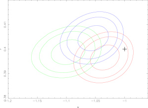
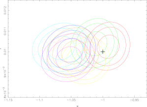
Figure 4: Parameter constraints obtained from full-sky lensed simulations using the $B$-mode power spectrum only and assuming Gaussianity. Contours are shown at the 67%, 95% and 99% confidence limits. Top: Model-A simulations. Bottom: Model-B simulations. The parameters in the fiducial model are marked with a cross.

We extracted the measured power spectrum $\hat{C}^{BB}_{\ell}$ of the simulations and constrained $r$ and $w$ with the likelihood appropriate to full-sky, noise-free observations of Gaussian fields:

$$P(\hat{\bm{C}}|\bm{C})\propto\prod_{\ell}\hat{C}_{\ell}^{\frac{2\ell-1}{2}}C_{\ell}^{-\frac{2\ell+1}{2}}\exp\left\{-\frac{(2\ell+1)\hat{C}_{\ell}}{2C_{\ell}}\right\},$$ (8)

where $C_{\ell}$ is the theoretical power spectrum. The normalisation of the likelihood function with respect to $\hat{C}_{\ell}$ is usually dropped since in practice it is a fixed quantity when constraining parameters. We assumed flat priors on the values of $w$ and $r$.

Figure 4 shows the parameter constraints obtained from three Model-A simulations and seven Model-B simulations using the likelihood in Eq. (8). It can be seen that the constraints are, in most cases, inconsistent with the input value of $w=-1$. However, the marginalised constraints on $r$ are in accordance with the input values. There appears to be a bias towards low values of $w$, and the spread of the maximum-likelihood values indicates that the constraints on $w$ are too tight. The latter is consistent with the findings of the Fisher analysis in Ref. Smith et al. (2004).

IV Non-Gaussian covariance

Equation (3) shows that the power in lensed $B$-modes on any particular scale arises from the power on a range of scales in $E$ and $\phi$. As can be seen in Fig. 1, the power in the lensing deflection field peaks at large scales, meaning that a significant fraction of the power in $B$-modes on scales around the peak is generated by large-scale lenses (see also Fig. 3). A particular mode in the lensing deflection field will lens many different $E$-modes to generate $B$-modes on a range of scales. The power in these $B$-modes will be related to the power in the single mode of the deflection field and so the measured power in $B$-modes is significantly correlated between scales Smith et al. (2004). In order to account for this non-Gaussianity in our analysis, we need to calculate the covariance between the measured $\hat{C}_{\ell}^{BB}$. The covariance can be expressed as a sum of the Gaussian and non-Gaussian parts:

$$\text{Cov}(\hat{C}^{BB}_{\ell_{i}},\hat{C}^{BB}_{\ell_{j}})=S_{ij}=S_{ij}^{\text{G}}+S_{ij}^{\text{NG}},$$ (9)

where the Gaussian part arises from the non-connected part of the $B$-mode four-point function and on the full sky is given by

$$S_{ij}^{\text{G}}=\delta_{ij}\frac{2(C_{\ell_{i}}^{BB})^{2}}{2\ell+1}.$$ (10)

Lensing has only a very small effect on any primordial $B$-modes from gravitational waves so we can treat these as an independent Gaussian field; their power spectrum then only enters the Gaussian part of the covariance matrix. Similar comments would apply to Gaussian instrument noise.

We can calculate the non-Gaussian part of the covariance matrix on the flat sky using the gradient approximation Eq. (2). The gradient approximation is not suitable for accurate calculation of the lensed power spectra (Lewis, 2005). In addition, the flat-sky approximation introduces per-cent level errors in the lensed $B$-mode spectrum on all scales Challinor and Lewis (2005). Fortunately, the errors from these approximations tend to cancel above $\ell\sim 400$ and the lensed $B$-mode spectrum can be computed to $\sim 1\%$ accuracy on such scales using Eq. (3). We anticipate that the non-Gaussian components of the covariance matrix computed with the gradient and flat-sky approximations will have a similar level of accuracy.

We thus calculate the non-Gaussian part of the covariance matrix within the flat-sky approximation using the bandpower expression given in Ref. Smith et al. (2004):

$$S^{\text{NG}}_{ij}=\frac{2}{A\alpha_{i}\alpha_{j}}\int_{\ell\in i}d^{2}\bm{\ell}_{i}\int_{\ell\in j}d^{2}\bm{\ell}_{j}\int\frac{d^{2}\bm{L}}{(2\pi)^{2}}\times$$

$$\left\{W^{2}(\bm{\ell}_{i},\bm{\ell}_{i}-\bm{L})W^{2}(\bm{\ell}_{j},\bm{\ell}_{j}-\bm{L})C^{\tilde{E}\tilde{E}}_{|\bm{\ell}_{i}-\bm{L}|}C^{\tilde{E}\tilde{E}}_{|\bm{\ell}_{j}-\bm{L}|}(C^{\phi\phi}_{L})^{2}\right.$$

$$+\;W^{2}(\bm{\ell}_{i},\bm{L})W^{2}(\bm{\ell}_{j},\bm{L})(C^{\tilde{E}\tilde{E}}_{L})^{2}C^{\phi\phi}_{|\bm{\ell}_{i}-\bm{L}|}C^{\phi\phi}_{|\bm{\ell}_{j}-\bm{L}|}$$

$$+\;W(\bm{\ell}_{i},\bm{\ell}_{i}-\bm{L})W(-\bm{\ell}_{i},\bm{\ell}_{j}-\bm{L})W(\bm{\ell}_{j},\bm{\ell}_{j}-\bm{L})$$

$$\left.W(-\bm{\ell}_{j},\bm{\ell}_{i}-\bm{L})C^{\tilde{E}\tilde{E}}_{|\bm{\ell}_{i}-\bm{L}|}C^{\tilde{E}\tilde{E}}_{|\bm{\ell}_{j}-\bm{L}|}C^{\phi\phi}_{L}C^{\phi\phi}_{|\bm{\ell}_{i}+\bm{\ell}_{j}-\bm{L}|}\right\},$$ (11)

where $A$ is the area of sky observed, $\alpha_{i}=\int_{\ell\in i}d^{2}\bm{\ell}_{i}$ and similarly for $\alpha_{j}$, and $W$ is given by Eq. (4). This expression assumes periodic boundary conditions both to remove the complications due to $E$-$B$ mixing and the additional correlations between the observed Fourier modes due to the geometry. For surveys of a few-hundred $\text{deg}^{2}$, the former should be negligible except on the largest scales, and the latter can be dealt with by choosing wide enough bands. Neither of these is an issue for the full-sky observations we consider here, and in this case we can set $A=4\pi$ and use bands of width $\Delta\ell=1$. This means that we can simplify this integral somewhat, since for a fixed length of $\bm{\ell}_{i}=\ell_{i}$ and $\bm{\ell}_{j}=\ell_{j}$ the value of the integrand is dependent only on the angle between $\bm{\ell}_{i}$ and $\bm{\ell}_{j}$ and their moduli. Therefore we can take out the integral over $\bm{\ell}_{j}$ and instead fix $\bm{\ell}_{j}=(\ell_{j},0)$. We can also simplify the integral over $\bm{\ell}_{i}$ to a one-dimensional integral in $\theta$. We can summarise this as

$$\frac{2}{A\alpha_{i}\alpha_{j}}\int_{\ell\in i}d^{2}\bm{\ell}_{i}\int_{\ell\in j}d^{2}\bm{\ell}_{j}\rightarrow\frac{1}{4\pi^{2}}\int_{0}^{2\pi}d\theta_{i}.$$ (12)

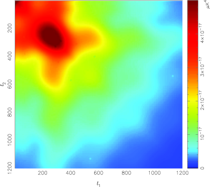
Figure 5: (Colour online) Illustration of the non-Gaussian component of covariance matrix $\mathrm{Cov}(\hat{C}^{BB}_{\ell_{1}},\hat{C}^{BB}_{\ell_{2}})$. The maximum value at the peak is $5\times 10^{-16}\mu$K⁴ but the scale has been set to illustrate the structure in the rest of the matrix more clearly.

Figure 5 illustrates the structure of the non-Gaussian component of the covariance matrix as calculated for Model A. It can be seen that the correlation is present across all scales and is not confined to the region near the diagonal. Although the non-Gaussian covariance between any two $\hat{C}_{\ell}^{BB}$ is small compared to the Gaussian covariance of the diagonal elements ($\sim 3\times 10^{-12}\,\mu\text{K}^{4}/\ell$ for $\ell\lesssim 300$), the fact that the non-Gaussian covariance spans a wide range of scales means that its net effect is very significant.

It is computationally expensive (taking several hours of CPU time) to re-calculate the covariance matrix for each set of model parameters as would be required in parameter estimation. However, when considering variations in those parameters that are not well constrained by the primary anisotropies ($w$ and $\Omega_{\nu}h^{2}$ here), the main effect on the lensed $B$-mode power spectrum is an overall scaling in amplitude. For this reason, we can approximate the covariance as

$$S_{ij}=S_{ij}^{\text{G}}+\frac{C_{\ell_{i}}}{C_{\ell_{i}}^{\mathrm{fid}}}\frac{C_{\ell_{j}}}{C_{\ell_{j}}^{\mathrm{fid}}}S_{ij}^{\text{NG,\,fid}},$$ (13)

where $C_{\ell}$ is the lensing contribution to the $B$-mode power spectrum and $C_{\ell}^{\text{fid}}$ is the same in the fiducial model. This is similar to the scheme suggested in Ref. Smith et al. (2004).

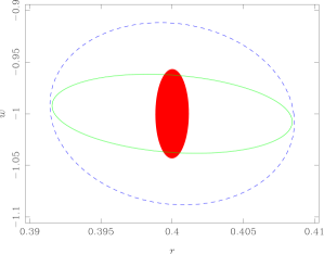
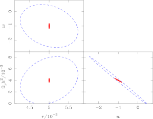
Figure 6: (Colour online) 95% confidence limits from a Fisher analysis. Top: Model A. Bottom: constraints for a model with same parameters as Model A except $r=0.005$ and $\Omega_{\nu}h^{2}=0.004$ (which we also allow to vary in the analysis). Blue dashed contours: limits if the lensed $B$-mode power spectrum is used, with the correct covariance matrix. Green solid line (top plot only): limits using the $B$-mode power spectrum and incorrectly assuming the data are Gaussian. Red filled area: theoretical limits if all unlensed power spectra are used including the power spectrum of the lensing deflection field.

We can calculate the theoretically-optimum constraints on parameters $\theta_{i}$ by performing a Fisher analysis. For Gaussian fields, the Fisher information matrix reduces exactly to Zaldarriaga and Seljak (1997)

$$F_{ij}=\sum_{\ell=2}^{\ell_{\mathrm{max}}}\sum_{X,Y}\frac{\partial C_{\ell}^{X}}{\partial\theta_{i}}\,\mathrm{Cov}^{-1}(C^{X}_{\ell},C^{Y}_{\ell})\,\frac{\partial C_{\ell}^{Y}}{\partial\theta_{j}},$$ (14)

where $X$ and $Y$ can be $TT$, $EE$, $TE$ or $BB$ and $\mathrm{Cov}^{-1}(C^{X}_{\ell},C^{Y}_{\ell})$ is the inverse covariance matrix of the various measured power spectra. If we wish to consider the information that can be obtained from the lensed $B$-mode power spectrum, we need to compute the Fisher matrix $-\langle\partial^{2}\ln P/\partial\theta_{i}\partial\theta_{j}\rangle$ where $P=P(\hat{C}_{\ell}^{BB}|\bm{\theta})$. If we can approximate this as Gaussian in the measured power spectrum, then provided the number of independent degrees of freedom is much larger than unity we find

$$F_{ij}\approx\sum_{\ell\ell^{\prime}}\frac{\partial C_{\ell}^{BB}}{\partial\theta_{i}}\,S^{-1}_{\ell\ell^{\prime}}\,\frac{\partial C_{\ell^{\prime}}^{BB}}{\partial\theta_{j}},$$ (15)

where $C_{\ell}^{BB}$ is the total $B$-mode power spectrum.

The tightest parameter constraints achievable under any circumstances from CMB data alone are those obtained from the power spectra of the unlensed, Gaussian, temperature and polarization fields together with the lensing deflection field. Some approximation to this situation may be achievable using the full likelihood function for the lensed CMB fields Hirata and Seljak (2003a); Hirata and Seljak (2003b), or, with larger errors, from quadratic reconstruction techniques Hu (2001); Hu and Okamoto (2002). In the top plot of Fig. 6 we show the constraints obtained from a Fisher analysis of Model A, if all parameter values are fixed except $r$ and $w$. We consider three cases: using only the lensed $B$-mode spectrum with the correct covariance matrix; the same but (wrongly) using only the Gaussian part of the covariance matrix; and using all of the unlensed CMB fields and the lensing deflection field (treated as Gaussian). In all cases we only kept modes up to $\ell=1200$. In the latter case, we include the unlensed CMB temperature and electric polarization though these have very little impact since the parameters we allow to vary are chosen to be nearly degenerate with respect to these fields. If the non-Gaussianity is neglected the constraints on $w$ from the $B$-mode power spectrum alone are slightly tighter than those obtainable using all of the unlensed fields, which shows immediately that we are making a false assumption Hu (2002). It can be seen that the errors on $r$ are almost unaffected by the non-Gaussianity whereas the errors on $w$ are significantly affected. However the presence of the lensed $B$-modes does significantly increase the errors on $r$ Knox and Song (2002); Kesden et al. (2002), so if the gravitational wave amplitude is small ($r\lesssim 0.01$) it will be desirable to attempt reconstruction of the unlensed CMB in order to detect the signal.

The degeneracy between $w$ and $\Omega_{\nu}h^{2}$ that is present when only the $B$-mode power spectrum is used can be clearly seen in the bottom plot of Fig. 6. Here, $r$, $w$ and $\Omega_{\nu}h^{2}$ are allowed to vary around a fiducial model with the same parameters as Model A except for a smaller $r=0.005$ and massive neutrinos with $\Omega_{\nu}h^{2}=0.004$. It should be recognised that a Fisher analysis, based on the derivatives of the power spectra around the fiducial model values, is good at highlighting degeneracies but does not give accurate error contours for degenerate parameters Eisenstein et al. (1999). The actual degeneracy between $w$ and $\Omega_{\nu}h^{2}$ follows a curve rather than a straight line. The degeneracy is broken by using the power spectrum of the lensing deflection field, although even then the variables are still correlated to a lesser extent. In the unlensed, foreground-free ideal case, the errors on $r$ are proportional to $r$ and so there is no lower limit to the value of $r$ that can be detected. In practice foreground residuals (and other systematic effects) are expected to pose a significant challenge and may well be the factor that limits the constraints that can ultimately be achieved.

V Non-Gaussian Likelihood

Having shown clearly that the non-Gaussianity of lensed $B$-modes cannot be ignored, we now address the question of how it may correctly be taken into account during parameter estimation from measured power spectra. To do this, we need to employ a likelihood function which includes information about the dependencies between the power on different scales. In principle, the exact likelihood can be found from that for the lensed fields Hirata and Seljak (2003a); Hirata and Seljak (2003b), but this would be very complicated, and such an analysis would probably be no simpler than an optimal analysis with the fields themselves (which would avoid the lossy compression to power spectra). Instead we proceed heuristically, modelling the likelihood as a function of the lensed spectrum and its covariance only. This necessarily assumes that the connected moments of the lensed field can be ignored above the four-point level, or, more correctly, that they can be approximated in a hierarchical manner by the lower moments. We only consider noise-free analysis on the full sky here, or, in Sec. VI, on a periodic flat sky. Since our approach is based on the measured power spectrum, the additional (geometric) complications from the survey geometry and those from instrument noise can be dealt with by standard techniques (see e.g. Challinor (2005)).

A suitable likelihood function must reduce to a good approximation to the true likelihood in the limit that the non-Gaussian covariance tends to zero, Eq. (8). Note that it is the dependence of this function on the cosmological parameters $\bm{\theta}$ that is of interest. The coupling of power between different scales by non-Gaussianity has a similar effect to the geometric coupling between scales that arises in observations of Gaussian fields over only part of the sky. A number of approximate likelihoods have been suggested for this latter problem, and a simple strategy for analysing lensed $B$-mode spectra might be to replace the (geometric) covariance matrix in these approximations by the non-Gaussian covariance matrix.

A possible first approximation, a likelihood function that is Gaussian in $\hat{C}_{\ell}$, is known to produce biased parameter constraints from Gaussian fields Bond et al. (2000). A better approximation is the log-normal distribution in which the likelihood is Gaussian in the log of the power. This was originally developed for the case where the peak of the likelihood (considered as a function of the theory $C_{\ell}$) and its curvature there are known Bond et al. (2000), but it can easily be tailored to our problem by replacing the modal $C_{\ell}$ by the measured $\hat{C}_{\ell}$, and the (inverse) curvature by the theoretical covariance matrix. (This likelihood was denoted by $\mathcal{L}_{\text{LN}}^{\prime}$ in Ref. Verde et al. (2003), with the prime distinguishing it from the original formulation in Ref. Bond et al. (2000); we make the same distinction in Eq. 16 below.) The log-normal likelihood has been employed in the analysis of several different CMB data sets, e.g. Goldstein et al. (2003); MacTavish et al. (2005); Pryke et al. (2002); Balbi et al. (2000); Rubiño-Martin et al. (2003). However, this likelihood is also biased; the level of bias is acceptable for many data sets but becomes significant when using full-sky data with a low noise level. The first-year WMAP data were analysed using a likelihood function which is a weighted combination of the Gaussian and log-normal likelihoods Verde et al. (2003):

$$\ln P(\hat{\bm{C}}|\bm{\theta})=\frac{1}{3}\ln P_{\mathrm{Gauss}}(\hat{\bm{C}}|\bm{\theta})+\frac{2}{3}\ln P^{\prime}_{\mathrm{LN}}(\hat{\bm{C}}|\bm{\theta}).$$ (16)

This is a significantly better approximation to the exact likelihood in the limit of no non-Gaussianity; see Fig. 10 of Appendix A for comparisons.

To illustrate the level of bias of the different likelihood functions when estimating $r$ and $w$, we created a Gaussian simulation of the CMB using the lensed $B$-mode power spectrum, and analysed the resulting measured power spectrum. The results are shown in Fig. 7. It can be seen that the constraints obtained when the WMAP likelihood function is employed are virtually indistinguishable from those obtained using the exact likelihood given by Eq. (8), although the Gaussian and log-normal approximations do lead to significant differences.

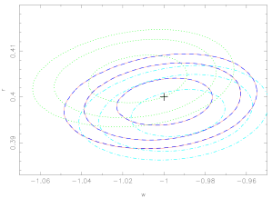
Figure 7: (Colour online) Likelihood contours at 67, 95 and 99% confidence limits from analysis of a Gaussian simulation of the CMB made using the lensed power spectrum. Red solid contours: using the exact likelihood function. Green dotted contours: using the Gaussian approximation to the likelihood function, showing the significant difference from the exact likelihood. Light blue dot-dashed contours: using the log-normal distribution, which gives a smaller, and opposite, shift. Dark-blue dashed contours: using the WMAP likelihood function, showing almost indistinguishable results from the exact likelihood. The fiducial model values are marked with a cross.

Figure 8 shows the marginalised distribution of $w$ obtained when the WMAP likelihood function is used to estimate parameters from the ten lensing simulations of Fig. 4. The non-Gaussian covariance matrix was included with the prescription in Eq. (13). Although from the spread of the maximum-likelihood values it seems that the width of the distributions are a good reflection of the uncertainties in the parameters, there is a significant bias towards low values of $w$, which means that, for most of the simulations, the parameter estimates are inconsistent with the input values. The marginalised distributions of $r$ are very similar to those obtained when Eq. (8) was applied to the same simulations. This indicates that the non-Gaussian contribution to the covariance is less significant on large scales, and hence the presence of non-Gaussianity does not introduce a bias, or affect the errors, on $r$. This is understandable since the signal which contains the information about $r$ is Gaussian to a high level.

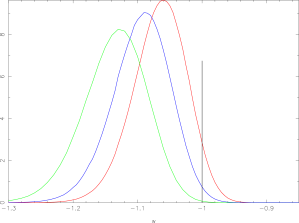
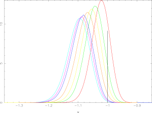
Figure 8: Marginalised distributions of $w$ obtained for three Model-A simulations (top) and seven Model-B simulations (bottom), using the WMAP likelihood function.

VI New likelihood function

In the previous section we showed that none of the existing likelihood approximations in the literature appear suitable for the analysis of future cosmic-variance limited, lensed $B$-mode data. For this reason we have re-examined the issue of likelihood approximations in CMB analysis; our findings can be found in Appendix A. The main result is a new likelihood function that appears to out-perform existing approximations. Here we summarise this new likelihood function and demonstrate that it produces accurate parameter constraints on simulated lensed data.

To begin, it is worth first reviewing the underlying issues that arise when constraining parameters from non-Gaussian fields. For ideal, full-sky observations, in the absence of non-Gaussianity, the probability of the observed fields $\bm{d}$ given the set of cosmological parameters $\bm{\theta}$ can be written as a function of the theoretical power spectrum $C_{\ell}(\bm{\theta})$ and the measured power spectrum $\hat{C}_{\ell}$:

$$P(\bm{d}|\bm{\theta})=P(\bm{d}|C_{\ell})=f(\hat{C}_{\ell})P(\hat{C}_{\ell}|C_{\ell}),$$ (17)

where $f(\hat{C}_{\ell})$ is a function of the measured power spectrum only. It follows that $\hat{C}_{\ell}$ are sufficient statistics for parameter estimation and hence there is no loss of information in compressing the data to the measured power spectrum. For non-Gaussian fields, even for ideal observations, the measured power is no longer a sufficient statistic and the likelihood may not just be a function of the theoretical power spectra of the fields. Nevertheless, we can regard the measured power spectrum as a form of lossy compression of the data, and the relevant likelihood is then the sampling distribution $P(\hat{C}_{\ell}|\bm{\theta})$.

In Appendix A we derive a new likelihood by approximating the properly-normalised distribution $P(\hat{C}_{\ell}|\bm{\theta})$ as Gaussian in some function of the $\hat{C}_{\ell}$. The likelihood takes the form

$$\ln P(\hat{C}_{\ell}|\bm{\theta})\approx\ln A-\frac{1}{2}\sum_{\ell\ell^{\prime}}M^{-1}_{\ell\ell^{\prime}}(\hat{x}_{\ell}-\mu_{\ell})(\hat{x}_{\ell^{\prime}}-\mu_{\ell^{\prime}}),$$ (18)

where

$$\hat{x}_{\ell} = \hat{C}_{\ell}^{1/3}$$ (19)

$$\mu_{\ell} = \left(\frac{2\ell-1}{2\ell+1}C_{\ell}\right)^{1/3},$$ (20)

and

$$M^{-1}_{\ell\ell^{\prime}}=3C_{\ell}^{2/3}\left(\frac{2\ell-1}{2\ell+1}\right)^{1/6}S^{-1}_{\ell\ell^{\prime}}\;3C_{\ell^{\prime}}^{2/3}\left(\frac{2\ell^{\prime}-1}{2\ell^{\prime}+1}\right)^{1/6},$$ (21)

where $S_{\ell\ell^{\prime}}$ is the covariance matrix of the measured $\hat{C}_{\ell}$ at parameters $\bm{\theta}$. The normalisation is

$$A^{-1}\propto\sqrt{\text{det}M_{\ell\ell^{\prime}}}\prod_{\ell}\mu_{\ell}^{2},$$ (22)

which we approximate here by $A\propto\prod_{\ell}1/C_{\ell}$. Note that the normalisation depends on the cosmological parameters and including this dependence is important to get an accurate approximation for the $\bm{\theta}$-dependence of the likelihood in the tails.

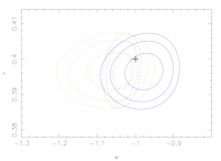
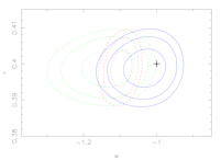
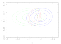
Figure 9: (Colour online) A comparison of the parameter constraints obtained for the three Model-A simulations, using different likelihood functions, with contours shown at 67, 95 and 99% confidence limits. Red dot-dash contours: constraints obtained assuming Gaussianity. Green dashed contours: using WMAP likelihood function. Blue solid contours: using new likelihood function. The fiducial model value is shown with a cross.

In Appendix A we show that this new likelihood is considerably more accurate than other approximations in current use when tested on full-sky, Gaussian data when the number of degrees of freedom is low (i.e. low $\ell$). When applied to Gaussian simulations, we find parameter constraints very similar to those shown for the WMAP (and exact) likelihood functions in Fig. 7. However, the new likelihood produces very different results when applied to non-Gaussian lensed simulations with the non-Gaussian covariance employed, as shown in Fig. 9. It can be seen here that for all three Model-A simulations the parameters constraints obtained are consistent with the values used in the simulations, unlike those obtained when the WMAP likelihood function is used. The results from the Model-B simulations are similar. In all cases the marginalised constraints on $r$ are nearly identical to those obtained when Gaussianity is assumed, which indicates that the non-Gaussianity does not noticeably affect the estimated value of $r$, although the presence of the lensed power spectrum itself does influence the bounds we can place on $r$. The parameter constraints are consistent with the theoretical errors obtained from the Fisher analysis shown in Fig. 6.

In order to test the new likelihood function further, we performed flat-sky lensed simulations, which can be computed much more rapidly than the full-sky simulations. It was found that, with a pixel size of 1.3 arcmin, accurate power spectra could be obtained by interpolation provided that a cubic interpolation method was used (a simple linear interpolation resulted in an inaccurate lensed power spectrum). Periodic boundary conditions were specified. The amplitude of the lensed $B$-mode power spectrum does not vary linearly with $w$, and for measured power spectra with large uncertainties, this results in a distribution of $w$ which is highly skewed and stretches far into the region $w<-1$. To avoid this, we used maps which were $91.7^{\circ}$ across to reduce the sample variance. It should be noted that for this size of map approximating the sky as flat is clearly incorrect; the statistics of the lensed modes in the simulations will differ at the per-cent level from the spherical expectations on all scales Challinor and Lewis (2005), and more so for those modes approaching the survey size. We performed 150 of these simulations, with Model-A parameters.

The estimated power spectrum of the flat-sky maps is calculated as bandpowers:

$$\hat{\mathscr{C}}_{i}=\frac{1}{A}\frac{\sum_{\bm{\ell}\in i}\ell^{2}|B(\bm{\ell})|^{2}}{2\pi\sum_{\bm{\ell}\in i}},$$ (23)

where $B(\bm{\ell})$ is the measured $B$-mode, the sum is over values of $\bm{\ell}$ that lie in band $i$, and, recall, $A$ is the area of the sky. In the limit that $\ell^{2}C_{\ell}/(2\pi)$ is constant within each band, we find that $\langle\hat{\mathscr{C}}_{i}\rangle=\ell^{2}C_{\ell_{i}}/(2\pi)$. The WMAP likelihood function can straightforwardly be generalised to work with bandpowers. For the new likelihood function we need to drop the $(2\ell-1)/(2\ell+1)$ factors; they are more significant at low-$\ell$ where the flat-sky approximation does not hold anyway. The bandpower version of the new likelihood function can then be expressed as

$$P(\hat{\mathscr{C}}|\bm{\theta}) \propto \frac{1}{\prod_{B}\mathscr{C}_{B}}\exp\Biggl{[}-\frac{1}{2}\sum_{BB^{\prime}}\left(\hat{\mathscr{C}}_{B}^{1/3}-\mathscr{C}_{B}^{1/3}\right)3\mathscr{C}_{B}^{2/3}$$ (24)

$$\mbox{}\times\;\mathcal{S}_{BB^{\prime}}^{-1}3\mathscr{C}_{B^{\prime}}^{2/3}\left(\hat{\mathscr{C}}_{B^{\prime}}^{1/3}-\mathscr{C}_{B^{\prime}}^{1/3}\right)\Biggr{]},$$

where the Gaussian part of the bandpower covariance matrix $\mathcal{S}_{B_{i}B_{j}}$ is given by

$$\mathcal{S}^{\text{G}}_{B_{i}B_{j}}=\delta_{ij}\frac{2(2\pi)^{2}}{A\alpha_{i}^{2}}\int_{\ell\in i}d^{2}\bm{\ell}\left(\frac{\ell^{2}}{2\pi}C_{\ell}^{BB}\right)^{2},$$ (25)

and the non-Gaussian part can be calculated from the non-Gaussian part of the the full-sky covariance matrix as:

$$\mathcal{S}^{\text{NG}}_{B_{i}B_{j}}=\frac{4\pi}{A}\frac{1}{\alpha_{i}\alpha_{j}}\sum_{\ell_{i}\in i}2\pi\ell_{i}\sum_{\ell_{j}\in j}2\pi\ell_{j}\frac{\ell_{i}^{2}\ell_{j}^{2}}{(2\pi)^{2}}S^{\text{NG,\,full}}_{\ell_{i}\ell_{j}}.$$ (26)

Since the posterior distribution of $w$ is skewed, as mentioned above, the maximum-likelihood value is greater than the mean value. Using the WMAP likelihood function, both the mean and maximum-likelihood values of $w$ were significantly biased, with values (averaged over the simulations) of $-1.075\pm 0.009$ and $-1.044\pm 0.007$ respectively. The quoted errors are standard errors in the mean of 150 simulations, and were estimated from the simulations. For both the mean and maximum-likelihood value, the bias is comparable to the random error on the measured value; the situation would worsen if we considered a larger survey area as the random error would fall but the bias would remain. Using the new likelihood, the mean of $w$ was $-0.992\pm 0.007$ and the maximum likelihood value $-1.017\pm 0.007$, showing that this likelihood function performs significantly better. A comparison between the width of the marginalised distributions of $w$ and the spread of the mean values estimated from each of the flat-sky simulations gave good agreement, to around one per cent. This shows that the estimated errors on the value of $w$ are correct once the non-Gaussian covariance is included. There was a slight positive bias in the mean of $r$ of about 0.5 per cent for the new likelihood and around twice this for the WMAP likelihood. This is about 30% of the random error on $r$ for the sample-variance limited observations considered here, but we expect that the bias is an artifact of the flat-sky simulations on large scales.

VII Conclusions

The generation of $B$-mode polarization by weak gravitational lensing provides a way of measuring cosmological parameters from the CMB alone that would otherwise be poorly constrained. We showed that a power spectrum analysis is wasteful, and in particular suffers from a strong degeneracy between the equation of state of the dark energy and neutrino masses. A more optimal analysis that reconstructs the lensing deflection field can break this degeneracy Kaplinghat et al. (2003), as can external data. Nevertheless, compression into the measured power spectrum will be a useful first step in the analysis of future $B$-mode data as it is likely to be more robust against real-world effects than more optimal reconstruction techniques. With this in mind, we have shown that it will be essential to take the non-Gaussianity of the lens-induced $B$-modes into account in a high signal-to-noise power-spectrum analysis, not only to avoid under-estimation of errors Smith et al. (2004) but also to remove biases in the parameters that affect lensing; constraints on the gravitational-wave amplitude are not noticeably affected by non-Gaussianity. Including the non-Gaussian covariance of the measured $B$-mode power spectrum in existing likelihood functions that have been used for parameter estimation from CMB spectra was shown to give biased results on noise-free simulations of lensed CMB fields. To remedy this we developed a new likelihood function that is more accurate in the tails of the distribution when the number of independent modes is low. Due to the non-Gaussian nature of CMB lensing, the number of such independent modes below a given multipole is lower than for Gaussian fields. We verified on simulations that the new likelihood function performs much better than existing approximations for the particular application considered here. However, we expect that it will be more generally applicable for the accurate analysis of the spectra of Gaussian CMB fields on large scales.

Appendix A Likelihood approximations

In this appendix we derive the likelihood approximation employed in Sec. VI. Our strategy for dealing with the non-Gaussianity of lens-induced $B$-mode data in this paper is heuristic: we include the non-Gaussian correlation between power on different scales but our choice of likelihood is motivated by the analysis of Gaussian fields. For this reason, our new likelihood approximation should also be useful more generally in CMB analysis. We only consider observations of a single field here ($\hat{C}_{\ell}^{B}$); we plan to address the more general problem of joint analysis of correlated fields in a future publication.

We develop two approximations motivated by the two ways that CMB power spectra are usually obtained. In the first, we work with the Gaussian CMB field $\bm{d}$ directly, and aim to characterise the probability $P(\bm{d}|C_{\ell})$ as a function of the theoretical power spectrum $C_{\ell}$ that encodes all of the cosmological information $\bm{\theta}$. Exploring $P(\bm{d}|C_{\ell})$ is computationally expensive so often the modal value of $C_{\ell}$ and the curvature (or a Fisher approximation to it) are found, e.g. Ref. Bond et al. (1998), and used in an analytic approximation to the $C_{\ell}$-dependence of $P(\bm{d}|C_{\ell})$. Complications due to, for example, the survey geometry, are accounted for only through their impact on the curvature matrix and modal $C_{\ell}$. We construct an approximate likelihood by looking for variables $x_{\ell}(C_{\ell})$ in which the exact likelihood is accurately represented by a Gaussian, i.e. we approximate the $C_{\ell}$-dependence of $\ln P(\bm{d}|C_{\ell})$ as

$$\ln P(\bm{d}|C_{\ell})\approx-\frac{1}{2}\sum_{\ell\ell^{\prime}}M^{-1}_{\ell\ell^{\prime}}(x_{\ell}-\mu_{\ell})(x_{\ell^{\prime}}-\mu_{\ell^{\prime}}),$$ (27)

up to an irrelevant constant. If this approximation is to peak at the correct place, we require $\mu_{\ell}=x_{\ell}(C_{\ell,{\text{ml}}})$, where $C_{\ell,{\text{ml}}}$ is the modal (or maximum-likelihood) value of $C_{\ell}$. Similarly, if the curvature at the peak is $-\mathcal{F}_{\ell\ell^{\prime}}$, we must have

$$M^{-1}_{\ell\ell^{\prime}}=\frac{\text{d}C_{\ell}}{\text{d}x_{\ell}}\frac{\text{d}C_{\ell^{\prime}}}{\text{d}x_{\ell^{\prime}}}\mathcal{F}_{\ell\ell^{\prime}},$$ (28)

where the derivatives are evaluated at the peak. To constrain the variable change $x_{\ell}(C_{\ell})$, we examine the third derivatives of $\ln P(\bm{d}|C_{\ell})$ with respect to the $x_{\ell}$:

$$\frac{\partial^{3}\ln P}{\partial x_{\ell}\partial x_{\ell^{\prime}}\partial x_{\ell^{\prime\prime}}} = \delta_{\ell\ell^{\prime}}\delta_{\ell\ell^{\prime\prime}}\frac{\partial\ln P}{\partial C_{\ell}}\frac{\text{d}^{3}C_{\ell}}{\text{d}x_{\ell}^{3}}$$ (29)

$$\mbox{}+\left(\delta_{\ell\ell^{\prime}}\frac{\partial^{2}\ln P}{\partial C_{\ell}\partial C_{\ell^{\prime\prime}}}\frac{\text{d}^{2}C_{\ell}}{\text{d}x_{\ell}^{2}}\frac{\text{d}C_{\ell^{\prime\prime}}}{\text{d}x_{\ell^{\prime\prime}}}+\text{cyclic perms.}\right)$$

$$\mbox{}+\frac{\partial^{3}\ln P}{\partial C_{\ell}\partial C_{\ell^{\prime}}\partial C_{\ell^{\prime\prime}}}\frac{\text{d}C_{\ell}}{\text{d}x_{\ell}}\frac{\text{d}C_{\ell^{\prime}}}{\text{d}x_{\ell^{\prime}}}\frac{\text{d}C_{\ell^{\prime\prime}}}{\text{d}x_{\ell^{\prime\prime}}},$$

where have imposed that $x_{\ell}$ is only a function of $C_{\ell}$ at the same $\ell$. Setting the right-hand side exactly equal to zero is, in general, inconsistent. Instead, we obtain a tractable and consistent problem if we demand that it vanish everywhere when we replace the derivatives of $P$ on the right with their expectation values evaluated with the likelihood appropriate to full-sky, noise-free observations Bond et al. (2000):

$$\ln P(\bm{d}|C_{\ell})=-\sum_{\ell}(\ell+1/2)(\hat{C}_{\ell}/C_{\ell}+\ln C_{\ell}),$$ (30)

where $\hat{C}_{\ell}$ is the measured $C_{\ell}$. Evaluating the expectation values of the derivatives of this likelihood (over data from an ensemble with power $C_{\ell}$), we find from Eq. (29) that we must have

$$4(\text{d}C_{\ell}/\text{d}x_{\ell})^{2}=3C_{\ell}\text{d}^{2}C_{\ell}/\text{d}x_{\ell}^{2}.$$ (31)

Note that the full-sky number of degrees of freedom $2\ell+1$ present in the derivatives cancels in this equation so we expect this procedure to remain valid for observations covering only a fraction $f_{\text{sky}}$ of the sky. Equation (31) is solved by $x_{\ell}=C_{\ell}^{-1/3}$, and gives an approximation for the $C_{\ell}$-dependence of $\ln P(\bm{d}|C_{\ell})$ of the form

$$\ln P(\bm{d}|C_{\ell}) = -\frac{1}{2}\sum_{\ell\ell^{\prime}}[3C_{\ell,\text{ml}}^{4/3}\mathcal{F}_{\ell\ell^{\prime}}3C_{\ell^{\prime},\text{ml}}^{4/3}$$ (32)

$$\mbox{}\times(C_{\ell}^{-1/3}-C_{\ell,\text{ml}}^{-1/3})(C_{\ell^{\prime}}^{-1/3}-C_{\ell^{\prime},\text{ml}}^{-1/3})],$$

up to an irrelevant constant. The essential difference with the log-normal approximation developed in Ref. Bond et al. (2000) is that they demand that the expectation of the curvature of the likelihood be constant (when approximated by Eq. 30) whereas we force the expectation value of the derivative of the curvature to be zero. These are not equivalent since the latter preserves the distinction between $C_{\ell,\text{ml}}$ and $C_{\ell}$ until after the derivative of the curvature is taken while the former does not.

To include instrument noise, we repeat the above steps but now include isotropic noise in the full-sky likelihood in Eq. (30). The effect in our approximate likelihood, Eq. (32), is to add a noise offset $N_{\ell}$ to $C_{\ell,\text{ml}}$ and $C_{\ell}$ in the right-hand side. Following Ref. Bond et al. (2000), we suggest determining $N_{\ell}$ by fitting the model

$$\mathcal{F}^{-1}_{\ell\ell}\approx\frac{2}{(2\ell+1)f_{\text{sky}}}(C_{\ell,\text{ml}}+N_{\ell})^{2},$$ (33)

to the diagonal elements of the inverse curvature at the peak.

The second approximation we consider is that which is used in Sec. VI. In this case, we first compress the data down to a measured power spectrum $\hat{C}_{\ell}$ and then ask what is the sampling distribution for the $\hat{C}_{\ell}$ given the cosmological model $\bm{\theta}$? We then use the $\bm{\theta}$-dependence of this probability as the likelihood in parameter estimation Wandelt et al. (2001). For noise-free observations of Gaussian fields over the full sky, the sampling distribution is given by Eq. (8) which on taking logs becomes

$$\ln P(\hat{C}_{\ell}|C_{\ell}) = -\sum_{\ell}\Big{(}\frac{2\ell+1}{2}\frac{\hat{C}_{\ell}}{C_{\ell}}+\frac{2\ell+1}{2}\ln C_{\ell}$$ (34)

$$\mbox{}\phantom{\sum_{\ell}}-\frac{2\ell-1}{2}\ln\hat{C}_{\ell}\Big{)},$$

up to a constant that is independent of $\hat{C}_{\ell}$ and the theoretical spectrum $C_{\ell}$. This approach is more natural for the non-Gaussian problem considered in the body of this paper since there we perform (lossy) compression down to $\hat{C}_{\ell}^{BB}$, and the power spectrum of the lensed $B$-modes does not fully characterise their statistics. We now look for a variable transformation $\hat{x}_{\ell}(\hat{C}_{\ell})$ in which the sampling distribution $P(\hat{C}_{\ell}|\bm{\theta})$ is approximately Gaussian:

$$\ln P(\hat{C}_{\ell}|\bm{\theta})\approx\ln A-\frac{1}{2}\sum_{\ell\ell^{\prime}}M^{-1}_{\ell\ell^{\prime}}(\hat{x}_{\ell}-\mu_{\ell})(\hat{x}_{\ell^{\prime}}-\mu_{\ell^{\prime}}),$$ (35)

where $A$ is a $\hat{C}_{\ell}$-independent (but cosmology-dependent) normalisation. We assume that we can calculate the mean $\langle\hat{C}_{\ell}\rangle$ and covariance $S_{\ell\ell^{\prime}}$ of the $\hat{C}_{\ell}$ given the cosmological model. Here we shall assume that $\hat{C}_{\ell}$ is constructed to be unbiased so $\langle\hat{C}_{\ell}\rangle=C_{\ell}$ although this assumption can easily be dropped. Since the mean and covariance of $P(\hat{C}_{\ell}|\bm{\theta})$ are specified rather than the modal value of $\hat{C}_{\ell}$ and the curvature there, we postpone their determination until we have determined the functional form of $\hat{x}_{\ell}$. This is obtained by examining the third derivatives of the sampling distribution with respect to $\hat{C}_{\ell}$. These are given by Eq. (29) but with $\hat{C}_{\ell}$ and $\hat{x}_{\ell}$ replacing $C_{\ell}$ and $x_{\ell}$. Again we approximate the derivatives with respect to $\hat{C}_{\ell}$, but this time with those derived from the distribution in Eq. (34). The second and third derivatives are independent of $C_{\ell}$ and we make no further approximation with these. We ignore the first derivative term since it is small near the peak, so, on setting the (approximate) third derivative of $\ln P$ with respect to $\hat{x}_{\ell}$ to zero, we find

$$2(\text{d}\hat{C}_{\ell}/\text{d}\hat{x}_{\ell})^{2}=3\hat{C}_{\ell}\text{d}^{2}\hat{C}_{\ell}/\text{d}\hat{x}_{\ell}^{2}.$$ (36)

This is solved by $\hat{x}_{\ell}=\hat{C}_{\ell}^{1/3}$. We could now determine $\mu_{\ell}$ and $M_{\ell\ell^{\prime}}$ by demanding that the approximate distribution gives the correct mean and covariance for $\hat{C}_{\ell}$. A simpler method, which we adopt here, is to relate $\mu_{\ell}$ and $M_{\ell\ell^{\prime}}$ to the (known) mean and covariance using Eq. (34) as a guide. For that ideal distribution, the peak is at $[(2\ell-1)/(2\ell+1)]\langle\hat{C}_{\ell}\rangle$ and the curvature at the peak is related to (minus) the inverse variance by a factor $[(2\ell+1)/(2\ell-1)]$. This motivates setting

$$\mu_{\ell} = \left(\frac{2\ell-1}{2\ell+1}C_{\ell}\right)^{1/3}$$ (37)

$$M^{-1}_{\ell\ell^{\prime}} = \sqrt{\frac{2\ell+1}{2\ell-1}}\frac{\text{d}\hat{C}_{\ell}}{\text{d}\hat{x}_{\ell}}S^{-1}_{\ell\ell^{\prime}}\sqrt{\frac{2\ell^{\prime}+1}{2\ell^{\prime}-1}}\frac{\text{d}\hat{C}_{\ell^{\prime}}}{\text{d}\hat{x}_{\ell^{\prime}}},$$ (38)

where the derivatives are taken at the peak where $\hat{x}_{\ell}=\mu_{\ell}$. If we use this to approximate the exact result Eq. (34) and evaluate the mean and standard deviation of $\hat{C}_{\ell}$, we find

$$\frac{\langle\hat{C}_{\ell}\rangle}{C_{\ell}} = 1+\frac{2}{27}\delta^{2}+\dots$$ (39)

$$\sqrt{\frac{2\ell+1}{2C_{\ell}^{2}}}\Delta\hat{C}_{\ell} = 1+\frac{1}{18}\delta+\dots,$$ (40)

where $\delta\equiv(\ell-1/2)^{-1}$. At $\ell=2$ the fractional error on the mean and standard deviation are 3% and 4% respectively; by $\ell=10$ these have dropped to $0.1\%$ and $0.6\%$. It remains to fix the normalisation. Exponentiating Eq. (35) and integrating with the approximation $\text{d}\hat{C}_{\ell}\approx 3\mu_{\ell}^{2}\text{d}\hat{x}_{\ell}$, we find that

$$A^{-1}\propto\sqrt{\text{det}M_{\ell\ell^{\prime}}}\prod_{\ell}\mu_{\ell}^{2},$$ (41)

where the proportionality constant is independent of the cosmological parameters $\bm{\theta}$. In the text we further approximate the normalisation by $A\propto 1/\prod_{\ell}C_{\ell}$.

To generalise our approximate sampling distribution to include instrument noise, we assume that the measured power spectrum has had a noise bias $N_{\ell}$ removed, so that $\langle\hat{C}_{\ell}\rangle=C_{\ell}$ still holds. The modifications we suggest are then $\hat{x}_{\ell}=(\hat{C}_{\ell}+N_{\ell})^{1/3}$ and replacing $C_{\ell}$ by $C_{\ell}+N_{\ell}$ in $\mu_{\ell}$.

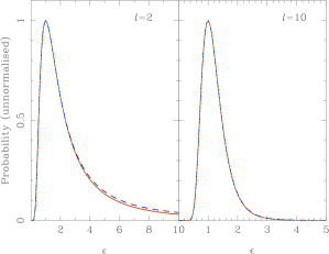
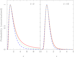
Figure 10: (Colour online) Comparison of likelihood approximations for $C_{\ell}$ for noise-free, full-sky observations of Gaussian fields. Left: the exact distribution (red, solid), Eq. (30); our new result (blue, dashed) in Eq. (32) that assumes the peak position and curvature there; and our alternative result (green, dotted) in Eq. (35) that works from the sampling distribution of the measured power spectrum, for $\ell=2$ (left panel) and $\ell=10$ (right panel). Note that the green dotted line is barely distinguishable from the exact distribution. Right: the log-normal distribution (blue, dashed); the WMAP likelihood (green, dotted) used in the analysis of the first-year data; and the exact likelihood (red, solid). In all cases $\epsilon\equiv C_{\ell}/\hat{C}_{\ell}$, where $\hat{C}_{\ell}$ is the measured $C_{\ell}$; $\hat{C}_{\ell}$ is also the maximum likelihood $C_{\ell}$ for the ideal conditions assumed.

In Fig. 10 we compare our two new likelihood approximations with the exact distribution, and also with the log-normal distribution proposed in Ref. Bond et al. (2000) and the likelihood used in the first-year WMAP analysis Verde et al. (2003), for the case of noise-free, full-sky observations of Gaussian fields. In this case, the measured power spectrum $\hat{C}_{\ell}$ equals the maximum likelihood spectrum $C_{\ell,\text{ml}}$, and working from the exact sampling distribution for $\hat{C}_{\ell}$ produces the same distribution for $C_{\ell}$ as working directly from the exact $P(\bm{d}|C_{\ell})$. Our new approximations are seen to be more accurate than the existing approximations, and particularly so when the number of degrees of freedom ($2\ell+1$ in this example) is small. Our second approximation, based on the sampling distribution of the measured $C_{\ell}$, is seen to be more accurate in the tail of the distribution than our first approximation that starts from the peak position and curvature. This appears to be because of the non-perturbative way in which the theoretical $C_{\ell}$ appear in the normalisation of the sampling distribution.