NGC 4435: a bulge dominated galaxy with an unforeseen low mass central black hole

Abstract

We present the ionised gas kinematics of the SB0 galaxy NGC 4435 from spectra obtained with the Space Telescope Imaging Spectrograph. This galaxy has been selected on the basis of its ground-based spectroscopy, for displaying a position velocity diagram consistent with the presence of a circumnuclear Keplerian disc rotating around a supermassive black hole (SMBH). We obtained the H$\alpha$ and [N II]$\,\lambda 6583$ kinematics kinematics in the galaxy nucleus along the major axis and two parallel offset positions. We built a dynamical model of the gaseous disc taking into account the whole bidimensional velocity field and the instrumental set-up. For the mass of the central SMBH we found an upper limit of $7.5\cdot 10^{6}$ M_⊙ at $3\sigma$ level. This indicates that the mass of SMBH of NGC 4435 is lower than the one expected from the $M_{\bullet}$$-$$\sigma_{c}$ ($5\cdot 10^{7}$ M_⊙) and near-infrared $M_{\bullet}$$-$$L_{\it bulge}$ ($4\cdot 10^{7}$ M_⊙) relationships.

1 Introduction

Over the last decade, kinematical studies have proved the presence of a supermassive black hole (hereafter SMBH) in the centre of about 40 galaxies of different morphological types. For a variety of reasons, SMBH are suspected to be present in the centres of all galaxies (see Ferrarese & Ford 2005 for a review).

The census of SMBHs is now large enough to probe the links between mass of SMBHs and the global properties of the host galaxies. The mass of SMBHs correlates with several properties of their hosting spheroid, such as the luminosity (Kormendy & Richstone 1995; Magorrian et al. 1998; Marconi & Hunt 2003), the central stellar velocity dispersion (Ferrarese & Merritt 2000; Gebhardt et al. 2000), the degree of light concentration (Graham et al. 2001), and the mass (Haring & Rix 2004). On the other hand, the SMBH masses do not correlate with the main properties of discs (Kormendy 2001), suggesting that formation of SMBHs is linked only to the formation of the spheroidal component of galaxies. The recent finding of a new correlation between the central stellar velocity dispersion and the rotational circular velocity (Ferrarese 2002; Baes et al. 2003; Pizzella et al. 2005) indicates that the mass of the SMBH could be also related to the mass of the dark matter halo.

The mass of SMBHs in elliptical and disc galaxies seems to follow the same scaling relations. However, accurate measurements of SMBH masses are available for only 11 disc galaxies (Ferrarese & Ford 2005) and the addition of new determinations for S0 and spiral galaxies are highly desirable. Reliable mass estimates of SMBHs in disc galaxies have been derived from observations of stellar proper motions in the Milky Way (Ghez et al. 2003) and spatially resolved kinematics of water vapor masers (Miyoshi et al. 1995), ionised gas (see Barth 2004 for a review) and stars (see Kormendy 2004 for a review) in the other galaxies. It is worth nothing that stellar proper motions can only be measured in our galaxy, water masers are not common and both the other two techniques offer merits and limitations. Stellar dynamical models are powerful as they give information not only on the mass of the SMBH but also on the orbital structure of the galaxy. However, both observational and computational requirements are expensive. The study of the ionised-gas kinematics represents a much easier way to trace the gravitational potential of galactic nuclei, since the orbital structure of the gas can be assumed to have a simple form, namely the one corresponding to a nearly Keplerian velocity field. However, the gas is more susceptible to non-gravitational forces and is often found in non-equilibrium configurations. Therefore the regularity of the ionised gas kinematics has to be verified observationally (Sarzi et al. 2001; Ho et al. 2002). The analysis of position-velocity diagrams (hereafter PVD) of the emission-line spectra observed with ground-based spectroscopy allows the identification of those galaxies which are good candidates for hosting a circumnuclear Keplerian disc (hereafter CNKD) rotating around a central mass concentration (Bertola et al. 1998). Their PVDs are characterized by a sharp increase of the velocity gradient toward small radii and the intensity distribution along the line shows two symmetric peaks with respect to the centre (Rubin et al. 1997; Sofue et al. 1998; Funes et al. 2002). These objects are good candidates for a spectroscopic follow-up with the Hubble Space Telescope (HST).

In this paper we present and model the ionised-gas kinematics of the SB0 galaxy NGC 4435 which we measured in spectra obtained with the Space Telescope Imaging Spectrograph (STIS). This is one of the galaxies we selected on the basis of ground-based spectroscopy, for displaying a PVD consistent with the presence of a CNKD rotating around a SMBH (Bertola et al. 1998). The paper is organized as follows. The criteria of galaxy selection are presented in Section 2. STIS observations are described and analyzed in Section 3. The resulting ionised-gas kinematics and the morphology of the dust pattern are discussed in Section 4. An upper limit for the SMBH mass of NGC 4435 is derived in Section 5. Finally, results are discussed in Section 7.

2 Sample selection

Our sample is constituted by three disc galaxies, namely NGC 2179, NGC 4343 and NGC 4435. We considered them as interesting targets for STIS because ground-based spectroscopic observations already allowed the determination of an upper limit for their SMBH mass, $M_{\bullet}$ (Bertola et al. 1998). Moreover, they are characterized by value of $\sigma_{c}$$\approx 150$ $\mathrm{km\;s}^{-1}$. This $\sigma_{c}$ value is lower than those of most of the galaxies so far studied with ionised-gas dynamics and higher than the few galaxies studied by means of water masers (Ferrarese & Ford 2005). For this reason, SMBH mass determinations in the proposed $\sigma_{c}$ range would allow a better comparison between data obtained either with gas or stellar dynamics. Finally, our sample galaxies belong to morphological types which are underrepresented in the sample of galaxies studied so far.

In this paper we present only the results of NGC 4435, since it is the only galaxy of our sample with smooth and circularly symmetric dust lanes as well as it is the only sample galaxy with a regular and symmetric velocity field of the ionised gas. This makes NGC 4435 an excellent candidate for the dynamical analysis. We defer discussion of both NGC 2179 and NGC 4343, as well as the estimate of the upper limit of their SMBH mass to a forthcoming paper (Corsini et al., in preparation).

NGC 4435 is a large (2.8 arcmin $\times$ 2.0 arcmin, [de Vaucouleurs et al. 1991, hereafter RC3]) and bright ($B_{T}=11.74$ [RC3]) early-type barred galaxy with intermediate inclination ($i=45^{\circ}$, from RC3 following Guthrie 1992). It is classified SB0⁰(s) and its total absolute magnitude is $M_{B}^{0}=-19.41$ (RC3), adopting a distance of 16 Mpc (Graham et al. 1999).

3 STIS observations and data reduction

The long-slit spectroscopic observations of NGC 4435 were carried out with STIS on March 2003 (Prog. Id. 9068, P.I. F. Bertola). STIS mounted the G750M grating centered at H$\alpha$ with the 0.2 arcsec $\times$ 52 arcsec slit. The detector was the SITe CCD with 1024 $\times$ 1024 pixels of 21 $\times$ 21 $\mu$m². No on-chip binning of the detector pixels yielded a wavelength coverage between about 6290 and 6870 Å with a reciprocal dispersion of 0.554 Å pixel^-1. The instrumental resolution was 1.6 Å (FWHM) corresponding to $\sigma_{\rm instr}\simeq 30$ $\mathrm{km\;s}^{-1}$ at H$\alpha$. The spatial scale was 0.05071 arcsec pixel^-1.

3.1 Acquisition images

Four HST orbits were allocated for observing the galaxy. At the beginning of the first orbit, two images were taken with the F28X20LP long-pass filter to acquire the nucleus. The acquisition images have a field of view of $5.4\times 5.4$ arcsec² and a pixel scale of 0.05071 arcsec. The exposure time was 40 s. The long-pass filter is centered at 7230 Å and has a FWHM$=2720$ Å. It roughly covers the $R$ band.

The first image was obtained by adopting for the nucleus the galaxy coordinates from the RC3 catalog. The image was boxcar-summed over a check box of $5\times 5$ pixels to find the position of the intensity peak. The flux-weighted centre of the brightest check box was assumed to be coincident with the nucleus location. This was used to recenter the nucleus and to obtain the second image. After determining the nucleus location, a small move was made to centre the nucleus in the slit. The acquisition images were bias-subtracted, corrected for hot pixels and cosmic rays, and flat-fielded using IRAF and the STIS reduction pipeline maintained by the Space Telescope Science Institute (Brown et al. 2002). Image alignment and combination were performed using standard tasks in the STSDAS package.

We used the resulting image to check the actual position of the slit during the spectroscopic observation as discussed in Section 3.3 and shown in Figure 1a. Moreover, this image was analyzed to map the dust distribution in the nuclear region of the galaxy. We constructed the unsharp-masked image using an identical procedure to Pizzella et al. (2002). We divided the image by itself after convolution by a circular Gaussian of width $\sigma=6$ pixels, corresponding to $0.30$ arcsec. This technique enhances any surface-brightness fluctuation and non-circular structure extending over a spatial region comparable to the $\sigma$ of the smoothing Gaussian. The resulting unsharp-masked image of NGC 4435 is given in Figure 1b.

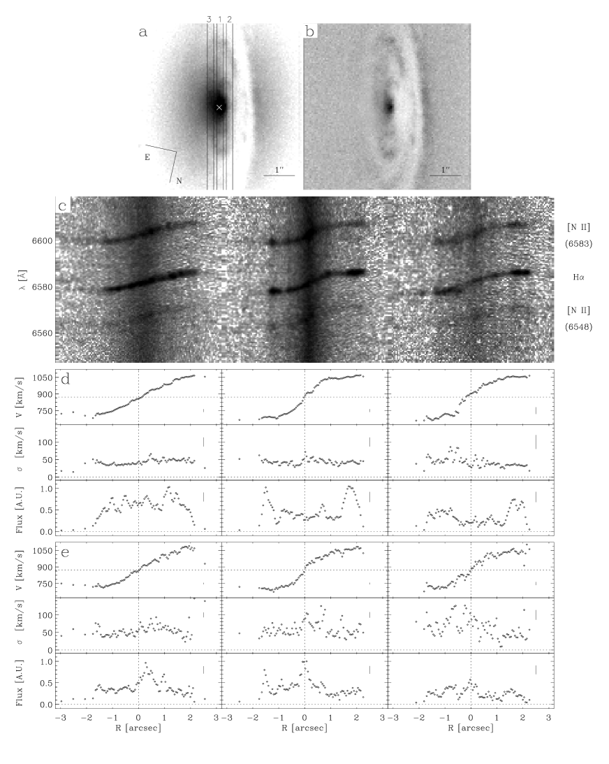
Figure 1: a) HST STIS/F28X20LP acquisition image of NGC 4435. The image has been rotated to the STIS instrumental frame. Orientation and scale are given. The white cross is the position of the nucleus from STIS acquisition procedure. The rectangles overplotted on the image show the actual locations of the slit during the spectroscopic observations. Table 1 lists the offsets of slit position 1, 2, and 3 with respect to the location of the nucleus. b) Unsharp-masking of the acquisition image of NGC 4435. c) Portions of the bidimensional STIS spectra of NGC 4435 obtained in position 1 (central panel), 2 (right panel) and 3 (left panel). The spectral region centered on the H$\alpha$ emission line is shown after wavelength calibration, flux calibration and geometrical rectification. The spatial axis is horizontal and ranges between $-3.2$ and $+3.2$ arcsec, while the wavelength axis is vertical and ranges from 6547 to 6619 Å. Individual emission lines are identified using a key, such that [N II] (6548), H$\alpha$, and [N II] (6583) correspond to [N II]$\,\lambda 6548$, H$\alpha$, and [N II]$\,\lambda 6583$, respectively. d) H$\alpha$ kinematics from the spectra of NGC 4435 obtained in position 1 (central panels), 2 (right panels) and 3 (left panels). For each slit position the line-of-sight velocity curve (top panel), the radial profile of the line-of-sight velocity dispersion (uncorrected for instrumental velocity dispersion, middle panel), and the radial profile of line flux in arbitrary units (bottom panel) are given. Errorbars are not plotted for clarity, but the typical errors are shown on the right side of each plot. e) Same as in d), but for the [N II]$\,\lambda 6583$ emission line.

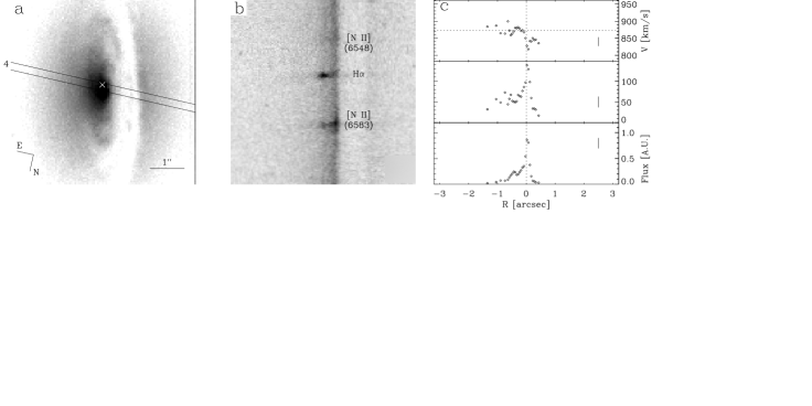
Figure 2: Similar to Figure 1, but for the archival spectrum of NGC 4435. The acquisition image of NGC 4435 with the slit location, a portion of the two-dimensional STIS spectrum after data reduction, and the [N II]$\,\lambda 6583$ kinematics are shown in panels a), b), and c), respectively. In a) the image orientation and scale is the same as in Figure 1a. In c) the spatial axis ranges between $-3.2$ and $+3.2$ arcsec, and the wavelength axis ranges from 6549 to 6627 Å.

3.2 Long-slit spectra

The position angle of the major axis of NGC 4435 is $\rm PA=13^{\circ}$ (RC3). We took STIS spectra of NGC4435 with the slit centered on the galaxy nucleus and located along its major axis, and with the slit parallel to the galaxy major axis on each side of its nucleus with an offset of $0.25$ arcsec. Following the target acquisition and peak up, 3 spectra were obtained with the slit along the major axis. Then the slit was offset westward by $0.25$ arcsec and 4 spectra were obtained in the first offset position. Finally, the slit was offset eastward by $0.5$ arcsec and 4 spectra were obtained in the second offset position. Observations of internal line lamps were obtained during each orbit for wavelength calibration. At each slit position, subsequent spectra were shifted along the slit by 5 detector pixels in order to remove the bad pixels. The total exposure time for each slit position was balanced within the constraints of a predefined HST offsetting pattern. The log of the observations with details about the spectra obtained for NGC 4435 are given in Table 1.

The spectra were reduced using the standard STIS reduction pipeline. The basic reduction steps included overscan subtraction, bias subtraction, dark subtraction, and flatfield correction. Subsequent reduction was performed using standard tasks in the STSDAS package of IRAF. Different spectra obtained for the same slit position were aligned using IMSHIFT and knowledge of the adopted shifts along the slit position. Cosmic ray events and hot pixels were removed using the task LACOS_SPEC by van Dokkum (2001). Residual bad pixels were corrected by means of a linear one-dimensional interpolation using the data quality files and stacking individual spectra with IMCOMBINE. We performed wavelength and flux calibration as well as geometrical correction for two-dimensional distortion following the standard reduction pipeline and applying the X2D task. This task corrected the wavelength scale to the heliocentric frame too. The contribution of the sky was determined from the edges of the resulting spectra and then subtracted. The resulting major-axis and offset spectra of NGC 4435 are plotted in Figure. 1c.

We found in the HST archive 3 other spectra of NGC 4435 which were taken in 1999 (Prog. Id. 7361, P.I. H.-W. Rix) with the same setup we adopted for our observations. These spectra were obtained with the slit placed across the galaxy nucleus with a position angle close to the galaxy minor axis (see Table 1). We retrieved the spectra and reduced them as explained above. The spectrum obtained close to the minor axis of NGC 4435 is shown in Figure 2c.

Table 1: Log of the STIS observations of NGC 4435. The number of spectra, nominal and actual offset, position angle, total exposure time, and observing date are listed for each slit position. Slit offsets are given with respect to the location of the target peak up.

Pos.	# Exp.	Nom. Of.	Act. Of.	PA	Exp. T.	Obs. Date
		(arcsec)	(arcsec)	(∘)	(s)
1	3	0	$+0.05$	12.5	3012	9 Mar 2003
2	4	$-0.25$	$-0.25$	12.5	3574	9 Mar 2003
3	4	$+0.25$	$+0.30$	12.5	3584	9 Mar 2003
4	3	0	$-0.08$	89.6	2673	26 Apr 1999

3.3 Location of the slits

In our observing strategy, the $0.2-$arcsec slit is centered on galaxy nucleus and it is aligned along the direction of the columns of the acquisition image at the end of target acquisition and peak up. The two subsequent offsets were done by applying shifts of $-0.25$ (i.e. westward) and $+0.5$ arcsec (i.e. eastward) in the direction of the rows of the acquisition image. In the archival spectra slit is nominally centered on galaxy nucleus.

We determined the actual location of the slits by comparing the light profile of the spectrum with the light profiles extracted from the acquisition image. We obtained the light profile of the spectrum by collapsing the spectrum along the wavelength direction over the spectral range between $6350$ and $6800$ Å. The comparison profiles were extracted from the acquisition image by averaging 4 adjacent columns. Each strip corresponds to a synthetic slit which is $0.2$ arcsec wide. Each slit position was determined with a $\chi^{2}$ minimization of the ratio between the light profile of the spectrum and the light profile extracted from the acquisition image.

We found that the slit centers were misplaced with respect to their nominal position. The difference between the nominal and actual positions of the slit centre with respect to intensity peak of the acquisition image is typically 1 STIS pixel. The locations of the slit are overlaid to the acquisition image in Figures. 1a and 2a, and the details about their positions are listed in Table 1.

3.4 Measurement of the emission lines

We derived the kinematics of the ionised-gas component by measuring the H$\alpha$ and [N II]$\,\lambda 6583$ emission lines, which are the strongest lines of the observed spectral range.

For each spectrum we extracted the individual rows out to a distance of about $2$ arcsec from the slit centre. At larger radii the intensity of the emission lines dropped off and we therefore binned adjacent spectral rows until a line signal-to-noise ratio $S/N\geq 10$ was attained. On each single-row extraction we determined the position, FWHM, and flux of the two emission lines by interactively fitting one Gaussian to each line plus a straight line to its local continuum. The non-linear least-squares minimization was done adopting the CURVEFIT routine in IDL. The centre wavelength of the fitting Gaussian was converted into heliocentric velocity in the optical convention $v=cz$. The Gaussian FWHM was converted into the velocity dispersion $\sigma$. The values of heliocentric velocity and velocity dispersion include no correction for inclination and instrumental velocity dispersion. Errors were calculated by taking into account Poisson noise, level of sky and continuum, read-out noise and gain of the CCD. The noise associated to the sky level, continuum level, and read out was estimated from a spectral region free of absorption and emission features after subtracting the fitted emission lines. For the archival spectrum of NGC 4435 we fitted only [N II]$\,\lambda 6583$ line because the H$\alpha$ line was so weak that little kinematic information could be derived from it.

Heliocentric velocities, velocity dispersions and fluxes measured from the H$\alpha$ and [N II]$\,\lambda 6583$ lines along the major and offset axes of NGC 4435, are plotted in Figures. 1d and 1e, respectively. Heliocentric velocities, velocity dispersions and fluxes measured close to the minor axis of NGC 4435 are given in Figure 2c.

4 Ionised-gas kinematics and dust morphology

The presence of a fairly-well defined nuclear disc of dust with relatively smooth and circularly symmetric dust rings and sharply defined edges is clearly visible in Figure 1b. It was first recognized in NGC 4435 by Ho et al. (2002).

We measured the H$\alpha$ and [N II]$\,\lambda 6583$ kinematics of NGC 4435 out to about 2 arcsec from the centre along the major and offset axes of NGC 4435 (Figures. 1d and 1e). The H$\alpha$ and [N II]$\,\lambda 6583$ velocity curves are regular and consistent within the errors. However, strong discrepancies are observed along the central slit for $0\la r\la 0.5$ arcsec, and along the western offset position for $-1\la r\la-0.5$ arcsec. We measured consistent values of velocity dispersion from the H$\alpha$ and [N II]$\,\lambda 6583$ lines, in spite of the larger scatter shown by the [N II]$\,\lambda 6583$ data.

We measured only the [N II]$\,\lambda 6583$ kinematics along the slit position close to the minor axis of NGC 4435 (Figure 2c). The measurements extend out to $\sim 1.5$ arcsec along the eastern side and to $\sim 0.5$ arcsec along the western side, where the dust lanes are more prominent. The minor-axis velocity curve and velocity dispersion profiles are strongly asymmetric. Our velocities are in agreement within the errorbars with those measured by Ho et al. (2002) by fitting simultaneously the H$\alpha$ and the two [N II] emission lines.

We note that along all slit positions the gas kinematics obtained from the H$\alpha$ and [N II]$\,\lambda 6583$ lines are too different to simply combine them in luminosity-weighted mean values. In particular, the H$\alpha$ rotation is characterised by a shallower velocity gradient than [N II]. Furthermore, most of the Ha flux appear to come from circumnuclear regions where low [N II]/H$\alpha$ ratios suggest star formation. On the other hand, the [N II] flux is much more concentrated toward the centre. Since the [N II] emission appears to probe better the nuclear regions and is characterised by a simpler flux distribution than H$\alpha$, we will take into account only the [N II] kinematics in our model.

NGC 4435 has smooth and circularly symmetric dust lanes as well as a regular and symmetric velocity field of the ionised gas. On the contrary, the other two galaxies of our sample are characterized by an irregular kinematics and an irregular dust lane morphology (Corsini et al., in preparation). This finding is in agreement with the results of Ho et al. (2002), that dust lanes can be used as relatively reliable predictor of the regularity of the gas kinematics in the nuclear regions of bulges. This makes NGC 4435 an ideal candidate for dynamical modeling.

5 Dynamical model

5.1 Velocity field modeling

5.1.1 Basic steps

A model of the gas velocity field is generated assuming that the ionised-gas component is moving onto circular orbits in an infinitesimally thin disc located in the nucleus of NGC 4435 around the SMBH. The model is projected onto the sky plane according to the inclination of the gaseous disc. Finally the model is “observed” simulating as close as possible the actual setup of STIS spectroscopic observations. The simulated observation depends on width and location (namely position angle and offset with respect to the centre) of each slit, STIS PSF and charge bleeding between adjacent CCD pixels. The mass of the SMBH is determined by finding the model parameters which produce the best match to the observed velocity curve. This modeling technique is similar to that adopted by Barth et al. (2001) and Marconi et al. (2003) to analyze STIS spectra obtained along parallel positions across the nucleus of NGC 3245 and NGC 4041, respectively.

5.1.2 Model calculation

Let $(r,\phi,z)$ be cylindrical coordinates and consider the gaseous disc in the $(r,\phi)$ plane with its centre in the origin. In the case of a spherical mass distribution, the gas circular velocity $v_{c}$ at a given radius $r$ is

$$v_{c}(r)=\left[\frac{GM(r)}{r}\right]^{1/2}=\left[\left(\frac{M}{L}\right)_{\star}v^{2}_{\star}(r)+\frac{GM_{\bullet}}{r}\right]^{1/2}$$ (1)

where $M$ is the total mass enclosed by the circular orbit of radius $r$, $(M/L)_{\star}$ is the (constant) mass-to-light ratio of the stellar component (and dark matter halo), and $v_{\star}$ is the circular velocity of radius $r$ for a stellar component with $(M/L)_{\star}$$=1$. The radial profile of $v_{\star}$ is derived from the observed surface-brightness distribution in Section 5.2.

The velocity dispersion of the gaseous disc is assumed to be isotropic with a Gaussian radial profile

$$\sigma(r)=\sigma_{0}+\sigma_{1}e^{-r^{2}/2r_{\sigma}^{2}}.$$ (2)

Unfortunately, H$\alpha$$+$[N II] imaging at HST resolution is not available for NGC 4435. This prevented us to build a map of the surface-brightness distribution of the ionised gas, as done for example in Barth et al. (2001). We therefore assume that the flux of the gaseous disc has an exponential radial profile

$$F(r)=F_{0}+F_{1}e^{-r/r_{F}}.$$ (3)

We now project the velocity field of the gaseous disc on the sky plane. Let $(x,y,z)$ be Cartesian coordinates with the origin in the centre of the gas disc, the $y$-axis aligned along the apparent major axis of the galaxy, and the $z$-axis along the line of sight directed toward the observer. The sky plane is confined to the $(x,y)$ plane. If the gaseous disc has an inclination angle $i$ (with $i=0^{\circ}$ corresponding to the face-on case), at a given sky point with coordinates $(x,y)$ the observed gas velocity $v(x,y)$ is

$$v(x,y)=v_{c}(x,y)\sin{i}\cos{\phi},$$ (4)

where

$$y = r\cos{\phi},$$ (5)

$$r = \left[\frac{x^{2}}{\cos^{2}i}+y^{2}\right]^{1/2}.$$ (6)

We assume that the velocity distribution of the gas at position $(x,y)$ is a Gaussian with mean $v(x,y)$, dispersion $\sigma(x,y)$, and area $F(x,y)$.

We now take into account the slit orientation. Let $(\xi,\eta,\zeta)$ be Cartesian coordinates with the origin in the STIS focal plane, the $\xi-$axis aligned with the direction of the slit width, $\eta$-axis aligned with the direction of the slit length and the $\zeta$-axis along the line of sight directed toward the observer and crossing the centre of the gas disc. The STIS focal plane corresponds to the $(\xi,\eta)$ plane. The $(x,y)$ and $(\xi,\eta)$ coordinate systems are related by the transformation

$$x = \xi\cos{\theta}-\eta\sin{\theta}$$ (7)

$$y = \xi\sin{\theta}+\eta\cos{\theta}$$ (8)

where $\theta$ is the angle between the slit direction and the disc major axis.

At position $(\xi,\eta)$ the flux contribution due to gas with a line-of-sight velocity $v$ in the range $[v-\delta v/2,v+\delta v/2]$ is given by

$$F(v|\xi,\eta)=\int_{v-\delta v/2}^{v+\delta v/2}\frac{F(\xi,\eta)}{\sigma(\xi,\eta)\sqrt{2\pi}}\exp{\frac{[v^{\prime}-v(\xi,\eta)]^{2}}{2\sigma(\xi,\eta)^{2}}}dv^{\prime}$$ (9)

where $\delta v$ is the velocity resolution of the model. For a given line-of-sight velocity $\hat{v}$, $F(\hat{v})$ is the “monochromatic” image of the gas velocity field observed at $\lambda=\lambda_{0}(1+\hat{v}/c)$ for a restframe wavelength $\lambda_{0}$.

The LOSVD predicted by the model at position $(\xi,\eta)$ on the focal plane is

$$S(v|\xi,\eta)=F(v|\xi,\eta)\otimes\mathrm{PSF}(\xi,\eta).$$ (10)

This takes into account the diffraction of light through the HST and STIS aperture.

For each position $\eta$ along the slit the LOSVD predicted by the model is given by the contribution of all the points on the focal plane inside the slit

$$S(v|\eta)=\int_{\xi_{c}-w/2}^{\xi_{c}+w/2}S(v+v_{d}M_{a}(\xi^{\prime}-\xi_{c})|\xi^{\prime},\eta)d\xi^{\prime}$$ (11)

where $\xi_{c}$ is the $\xi$ position of the slit centre, $w$ is the slit width, $v_{d}$ is the velocity bin along the wavelength direction in the spectral range of interest, and $M_{a}$ is the anamorphic magnification factor which accounts for the different scale in the wavelength and spatial direction on the focal plane. For STIS in the observed spectral range $v_{d}=25.2$ $\mathrm{km\;s}^{-1}$ pixel^-1. The scale in the wavelength direction is $0.05477$ arcsec pixel^-1 and the scale in the spatial direction is $0.05071$ arcsec pixel^-1, thus $M_{a}=0.93$ (Bowers & Baum 1998). The velocity offset $v_{d}M_{a}(\xi-\xi_{c})$ is the shift due to the nonzero width of the slit and its projection onto the STIS CCD. The difference $\xi-\xi_{c}$ is in pixel units since $v_{d}$ is given in $\mathrm{km\;s}^{-1}$ pixel^-1. The velocity offset accounts for the fact that the wavelength recorded for a photon depends on the position $\xi-\xi_{c}$ at which the photon enters the slit along the $\xi$ axis (Maciejewki & Binney 2001; Barth et al. 2001). This effect is sketched in Figure 3.

Figure 3: Schematic representation of the velocity shift caused by the non zero width of the slit. The spectra generated along the slit width in pixels of coordinates $(\xi_{1},\eta)$, $(\xi_{2},\eta)$, $(\xi_{3},\eta)$, and $(\xi_{4},\eta)$ are characterized by a velocity offset $\Delta v(\xi_{i}-\xi_{c})$, where $i=1,2,3,4$ and $\xi_{c}$ corresponds to the slit centre. The resulting spectrum is $S(v|\eta)$.

We performed a summation over pixels rather than an integration of analytic functions. The model LOSVD and the STIS PSF were calculated on a subsampled pixel grid with the bin size of $\delta s=0.01268\times 0.01268$ arcsec² (i.e., a subsampling factor $4\times 4$ relative to the STIS pixel scale) and on a velocity grid with bin size of $\delta v=10$ $\mathrm{km\;s}^{-1}$. $\delta s$ and $\delta v$ correspond to spatial and velocity resolution of the model calculation, respectively. In principle, smaller values for $\delta s$ and $\delta v$ could give a more accurate model calculation, but do not increase the result accuracy. The adopted values are the best comprise between good sampling and reasonable computational time (300 s on a 1-GHz PC). We generated the PSF for a monochromatic source at 6600 Å using the TINY TIM package in IRAF (Krist & Hook 1999). Convolution with the PSF is done using the fast Fourier transform algorithm (Press et al. 1992).

The model LOSVD was rebinned on a spatial grid with the bin size of $0.05701\times 0.05701$ arcsec² and on a velocity grid with the bin size of $v_{d}=25.2$ $\mathrm{km\;s}^{-1}$ to match the STIS pixel scale in the spatial and wavelength direction, respectively. For each slit position, the array of model LOVSDs forms a synthetic spectrum which is similar to the STIS spectrum. It was convolved with the CCD-charge diffusion kernel given by Krist & Hook (1999) in order to mimic the bleeding of charges between adjacent STIS CCD pixels.

Finally, we analyzed the synthetic spectrum as the STIS spectra and measured line-of-sight velocity $v_{\it mod}$, velocity dispersion $\sigma_{\it mod}$, and flux $F_{\it mod}$ as a function of radius.

5.2 Stellar component

To investigate the central mass concentration of NGC 4435 it is necessary to determine the contribution of the stellar component to the total potential (see Eq. 1).

5.2.1 WFPC2 imaging

We retrieved Wide Field Planetary Camera 2 (WFPC2) images of NGC 4435 from the HST archive. Data for the filter F450W and F814W (Prog. Id. 6791, P.I. J. Kenney) were selected to determine the stellar light profile minimizing the effects of dust absorption. Two images are available for both filters. Total exposure times were 600 s and 520 s with the F450W and F814W filter, respectively. All exposures were taken with the telescope guiding in fine lock, which typically gave an rms tracking error of $0.003$ arcsec. We focused our attention on the Planetary Camera chip (PC) where the nucleus of the galaxy was centered for both the filters. This consists of $800\times 800$ pixels of $0.0455\times 0.0455$ arcsec² each, yielding a field of view of about $36\times 36$ arcsec².

The images were calibrated using the standard WFPC2 reduction pipeline maintained by the Space Telescope Science Institute. Reduction steps include bias subtraction, dark current subtraction, and flat-fielding are described in detail in Holtzman et al. (1995). Subsequent reduction was completed using standard tasks in the STSDAS package of IRAF. Bad pixels were corrected by means of a linear one-dimensional interpolation using the data quality files and the WFIXUP task. Different images of the same filter were aligned and combined using IMSHIFT and knowledge of the offset shifts. Cosmic ray events were removed using the task CRREJ. The cosmic-ray removal and bad pixel correction were checked by inspection of the residual images between the cleaned and combined image and each of the original frames. Residual cosmic rays and bad pixels in the PC were corrected by manually editing the combined image with IMEDIT. The sky level ($\sim 1$ count pixel^-1) was determined from regions free of sources in the Wide Field chips and subtracted from the PC frame after appropriate scaling.

Flux calibration to Vega magnitudes was performed using the zero points by Whitmore (1995). To convert to standard $B$ and $I$ filters in the Johnson system, we estimated the color correction using the SYNPHOT package of IRAF with the S0 spectrum from Kinney et al. (1996) as template. The color corrections are $B-{\rm F450W}=+0.115$ and $I-{\rm F814W}=-0.119$.

5.2.2 Correction of dust absorption

We attempted to correct the data for the effects of dust absorption using a method similar to the one described in Cappellari et al. (2002).

For each galaxy pixel we measured the $B-I$ color and we derived the length $a$ of the semi-major axis of its elliptical isophote. The average position angle ($\theta=17^{\circ}$) and ellipticity ($\epsilon=0.66$) of the dust features were derived from the analysis of the unsharp-masked STIS acquisition images as discussed in Section 5.3. We assumed that the intrinsic galaxy color varies linearly as a function of radius. This assumption is justified by Figure 4 which shows the intrinsic galaxy color $(B-I)_{0}$ obtained as a straight-line fit to the pixel color as a function of $a$. For each pixel we computed the color excess $E(B-I)$ as difference between the measured color $B-I$ and the intrinsic galaxy color $(B-I)_{0}$ fitted at that radius. This allowed us to obtain a $E(V-I)$ map of the nuclear region of NGC 4435. The result is shown in Figure 5. We computed the $A(I)=0.558E(B-I)$ using the standard Galactic extinction curve given by Cardelli et al. (1989) with the assumption that the observed color gradient is due to dust rather than stellar population. We assumed that dust is distributed in an uniform screen in front of the galaxy and we used the $A(I)$ map to correct the $I-$band image for extinction. The extinction-corrected image is shown in Figure 5. We applied the $A(I)$ correction only to pixels with $|E(B-I)|$ above a given threshold. By comparing the pixel color in the eastern and western sides of the galaxy, we defined the threshold as $2$ times the standard deviation of the observed color with respect to the intrinsic one. We calculated the threshold for $4<a<15$ arcsec and extrapolated it for $a\leq 4$ arcsec to account for the increasing dust absorption at smaller radii (Figure 4).

This method corrects the major effects of patchy dust absorption. Nevertheless, the dust disc is still visible in the corrected image, although it is much less optically thick than in the original one.

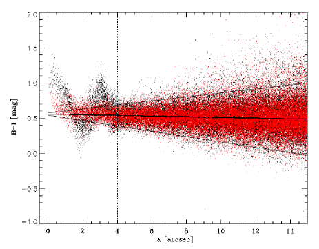
Figure 4: Calibrated Johnson $B-I$ color for every pixel in the WFPC2 image of NGC 4435 as a function of its elliptical radius $a$. Black and red dots refer to pixel on the eastern and western side of the galaxy, respectively. The thick and two thin continuous lines correspond to fitted intrinsic color $(B-I)_{0}$ and $E(B-I)$ thresholds, respectively. Thresholds have been derived for pixels at $4<a<15$ arcsec and extrapolated to the innermost radii.

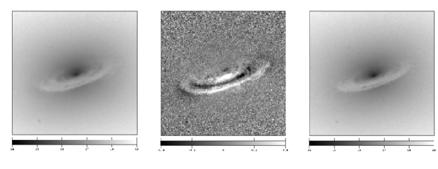
Figure 5: Dust correction of the WFPC2/F814W image of NGC 4435. Left panel: Observed WFPC2/F814W image after calibration to Johnson $I-$band. Middle panel: Map of the color excess $E(B-I)$. Right panel: Extinction-corrected $I-$band image. The field of view is $10.6\times 10.6$ arcsec² and the color scale is given in magnitudes.

5.2.3 Stellar density profile

Surface photometry was derived on the $I-$band extinction-corrected image by performing an isophotal analysis with the IRAF task ELLIPSE. We derived the isophotal profiles of the galaxy by first masking out the remaining dust patches and then fitting ellipses to the isophotes. We allowed the centres of the ellipses to vary, to test whether the light distribution in galaxy nucleus was still affected by dust obscuration. Since we found some evidence of variations in the fitted centre, the ellipse fitting was repeated with the ellipse centres fixed to the location found for the outermost isophotes. The resulting azimuthally averaged surface-brightness, ellipticity, and position angle radial profiles are presented in Figure 6.

Figure 6: Radial profiles of Johnson $I-$band surface brightness (top panel), ellipticity (middle panel), and position angle (bottom panel) measured on the extinction-corrected image of NGC 4435.

The isophotes of the masked image are quite circular with $\epsilon\la 0.3$ (Figure 6). For $r<9$ pc (2.5 pixels) the ellipticity is poorly estimated due to the limited pixel sampling. This allowed us to treat the surface-brightness distribution as circularly symmetric, and to assume the stellar density distribution as spherically symmetric. This approximation is sufficient to estimate the mass-to-light ratio in the radial range where the ionised-gas kinematics probes the galaxy potential.

We derived the radial profile of the deprojected stellar luminosity density $\Gamma(r)$ from the radial profile of the observed surface-brightness profile $\Sigma(R)$. The intrinsic surface-brightness profile of the galaxy $S(R)$ and image PSF were modeled as a sum of Gaussian components using the Multi Gaussian Expansion (MGE hereafter) described by Monnet et al. (1992) as done by Sarzi et al. (2001). The PSF for the WFPC2/F814W image was generated using the TINY TIM package in IRAF (Krist & Hook 1999). The multi-Gaussian $S(R)$ was convolved with the multi-Gaussian PSF and then compared with $\Sigma(R)$ to obtain optimal scaling coefficients for the Gaussian components. The Gaussian width coefficients were constrained to be a set of logarithmically spaced values, thus simplifying the MGE into a general non-negative least-squares problem for the corresponding Gaussian amplitudes. For a spherical light distribution, the MGE method leads to a straightforward deprojection of $S(R)$ into the deprojected stellar luminosity density $\Gamma(r)$, which can be also expressed as the sum of set of Gaussians.

For a spherical mass distribution and a radially constant mass-to-light ratio, $(M/L)_{\star}$, the stellar mass density $\rho(r)$ can be expressed as $\rho(r)=$$(M/L)_{\star}$$\Gamma(r)$. It is the sum of spherical mass components whose potential can be computed in term of error functions. The circular velocity $v_{\star}$(r) to be used in Eq. 1 is derived assuming $(M/L)_{\star}$$=1$. The multi-Gaussian fit to observed surface-brightness profile is shown in Figure 7 along with the recovered luminosity density profile, and the corresponding circular velocity curve for $(M/L)_{\star}$$=1$.

We note that since both B and I-band images are affected by dust, the B-I maps can only deal a limited description for the dust distribution. Unfortunately near-IR images of high spatial resolution for NGC 4435 do not exist. The use of such images would likely lead to find a larger amount of dust absorption than presently estimated. Hence, we are currently underestimating the contribution of the stars to the total mass, and overrating the SMBH mass. The use of the B-I colour will therefore not affect our conclusions.

Figure 7: Deprojection steps for the stellar mass profile of NGC 4435. Top panel: Multi-Gaussian fit to observed surface-brightness profile. Middle panel: Deprojected stellar luminosity density profile. Bottom panel: Circular velocity curve that results if the stellar mass and luminosity density are proportional with $(M/L)_{\star}$$=1$. In each panel the dashed lines correspond to the $1\sigma$ confidence limits.

5.3 Orientation of the gaseous disc

The prediction of the observed gas velocity field for NGC 4435 depends on the orientation of the nuclear gaseous disc, which can be different from that of the main galaxy disc.

We therefore modeled the gas kinematics by constraining the position angle $\theta$ and inclination $i$ of the gaseous disc under the assumption that the dust lanes are a good tracer of the orientation of the gaseous disc (Sarzi et al. 2001). We estimated $\theta$ and $i$ by defining ellipses consistent with the morphology of the dust pattern (as observed in Figure 1b) and assuming that dust lanes are circularly symmetric. Although the strength of the dust lanes varies spatially, it is possible to identify the two most conspicuous ones by visual inspection of the unsharp-masked version of the STIS acquisition image. To constrain the orientation of the gaseous disc we selected two of these features. The inner one has a semi-major axis of $\sim 2$ arcsec, which corresponds to the maximum extent of our kinematic measurements, and the outer one marks out the edge of dust pattern on the western side of the galaxy.

In each row of the unsharp-masked acquisition image we determined the position of the two main dust lanes by interactively fitting one Gaussian to each absorption feature plus a straight line to its local starlight continuum on both side of the nucleus. Once determined the position of the dust lanes, we fitted them with two ellipses with same centre (Figure 8). The non-linear least-squares minimization was done adopting the CURVEFIT routine in IDL. The ellipses have different position angles ($\theta_{\it in}=17.0^{\circ}\pm 1.0^{\circ}$, $\theta_{\it out}=13.8^{\circ}\pm 0.5^{\circ}$) but same ellipticity ($\epsilon_{\it in}=\epsilon_{\it out}=0.66\pm 0.03$). The different position angles of the two ellipses can be interpreted as indicative of a slightly warped gaseous disc, but this does not affect the final results of the dynamical model as discussed in Section 5.4. We assumed for the gaseous disc $\theta=17^{\circ}\pm 1^{\circ}$ and $i=70^{\circ}\pm 2^{\circ}$, since the measured kinematics are encircled by the ellipse corresponding to the inner dust lane.

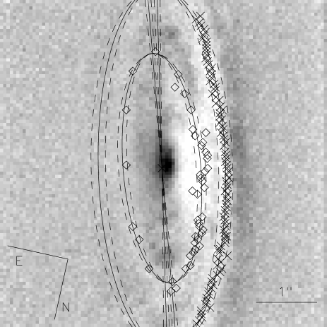
Figure 8: The orientation of the gaseous disc of NGC 4435. Diamonds and crosses corresponding to the points of the inner and outer dust lanes are overplotted to Figure 1b. Absorption features are brighter in this unsharp-masked image. The best-fit ellipses of the inner and outer dust lanes and their position angles are shown with solid ellipses and solid lines, respectively. The dashed ellipses and dashed lines enclose the 1$\sigma$ confidence ranges on best-fit ellipticity and position angle for both the isophotes.

5.4 Best-fitting model

The parameters in our model are the mass $M_{\bullet}$ of the SMBH, the mass-to-light ratio $(M/L)_{\star}$ of the stellar component (and dark matter halo), the inclination $i$ and position angle $\theta$ of the gaseous disc, the parameters $\sigma_{0}$, $\sigma_{1}$, and $r_{\sigma}$ of the Gaussian radial profile of the intrinsic velocity dispersion of the gas ( see Eq. 2), and the parameters $F_{0}$, $F_{1}$, and $r_{F}$ of the exponential radial profile of the gas flux ( see Eq. 3). Given the large number of parameters, it is highly desirable to constrain as many as possible of them. We started by fixing the orientation of the gaseous disc using the results of the analysis of the dust lanes of Section 5.3. We therefore assumed $\theta=17^{\circ}$ and $i=70^{\circ}$ to model the gas velocity field.

We initially considered a grid of models in which every point is determined by $M_{\bullet}$ and $(M/L)_{\star}$. For every model in this grid we explored several combination for $\sigma_{0}$, $\sigma_{1}$, $r_{\sigma}$, $F_{0}$, $F_{1}$, and $r_{F}$ in order to match the observations. This preliminary analysis revealed that the predicted flux profile does not depend on the input values of $M_{\bullet}$ and $(M/L)_{\star}$, while the velocity dispersion profile depends only on the adopted value of $M_{\bullet}$. The flux parameters need to be adjusted only if different disc orientations are considered. This means that we can adopt the same flux parameters ($F_{0}$, $F_{1}$, and $r_{F}$) for every point of the grid, but we need to adjust the velocity dispersion parameters ($\sigma_{0}$, $\sigma_{1}$, $r_{\sigma}$) depending on the value the black hole mass $M_{\bullet}$. Therefore, we can find the optimal values for $F_{0}$, $F_{1}$, and $r_{F}$ at any position in the $M_{\bullet}-(M/L)_{\star}$ grid, by minimizing the $\chi^{2}_{F}=\sum(F-F_{\it mod})^{2}/\delta F^{2}$ where $F\pm\delta F$ and $F_{\it mod}$ are the observed and the corresponding model flux along the major axis (the other slit positions are not reproducible). The best-fitting values are $F_{0}=0.08$ and $F_{1}=0.61$ in the adopted arbitrary units and $r_{F}=10$ pc. The velocity dispersion parameters need to be optimized for every value of the $M_{\bullet}$ in the grid, by minimizing the $\chi^{2}_{\sigma}=\sum(\sigma-\sigma_{\it mod})^{2}/\delta\sigma^{2}$ where $\sigma\pm\delta\sigma$ and $\sigma_{\it mod}$ are the observed and the corresponding model velocity dispersion along the different slit positions, respectively. The values of the adopted parameters for different $M_{\bullet}$ values are listed in Table 2. Although the velocity dispersion parameters depend only mildly on the disc orientation, we changed them when considering different orientations than the one traced by the dust lanes (Section 6.2).

We then explored a grid of models with $0\leq M_{\bullet}\leq 1.25\cdot 10^{7}$ M_⊙ and $2.0\leq(M/L)_{\star}\leq 2.35$ (M/L)_⊙, where at every point of the grid we now use the optimized parameters for the flux and velocity dispersion obtained before. For each model we calculated the $\chi^{2}=\sum(v-v_{\it mod})^{2}/\delta^{2}(v)$ where $v\pm\delta(v)$ and $v_{\it mod}$ are the observed and the corresponding model velocity along the different slit positions. The best model has $\chi^{2}=955$ and a reduced $\tilde{\chi}^{2}=5.2$. The best-fitting model requires no $M_{\bullet}$ and is compared to the observed [N II]$\,\lambda 6583$ kinematics in Figure 11. As we cannot reproduce the observed wiggles and asymmetries, which could be due to the patchiness of the surface-brightness distribution of the gas (Barth et al. 2001), in a strict $\chi^{2}$ sense our best match is not a good model. Before deriving confidence limits on $M_{\bullet}$ and $(M/L)_{\star}$, we therefore need to allow for the velocity structures that are not reproduced by rescaling all $\chi^{2}$ values in order for the best $\chi^{2}$ to match the number of degree of freedom $N-M$, where $N=184$ is the number of the observed points and $M=2$ is the number of the parameters in our model. Note that this procedure is equivalent to allowing for an additional source of error in our data and leads to more conservative confidence intervals. Figure 9 show 1$\sigma$, 2$\sigma$, and 3$\sigma$ confidence levels on $M_{\bullet}$ and $(M/L)_{\star}$ alone, according to the $\Delta\chi^{2}$ variations expected for one parameter (i.e. 1, 3, and 9; Press et al. 1992). Figure 10 shows similar confidence regions for $M_{\bullet}$ and $(M/L)_{\star}$ jointly, according to the $\Delta\chi^{2}$ variation expected for two parameters (i.e. 2.4, 6.2, 11.8). For the SMBH in NGC 4435 we derived an upper limit $M_{\bullet}\leq 7.5\cdot 10^{6}$ M_⊙ at 3$\sigma$ confidence level. The mass-to-light ratio is $(M/L)_{\star}$$=2.20^{+0.10}_{-0.12}$ at 3$\sigma$ confidence level. The sampling of the grid in the parameters spaces is $2.5\times 10^{6}M_{\odot}$ for the SMBH mass, and 0.05 (M/L)_⊙ for the mass-to-light ratio. The previous results do not change significantly if we use a grid with a smaller sampling step.

As stated before, according to the $\chi^{2}$ analysis the model is not sophisticated enough to reproduce the data wiggles. However to mitigate this problem we can rebin the kinematics in the outermost regions (beyond $|R|>0.5$ arcsec, where the influence of the SMBH is negligible). The errors on every re-binned data were computed as the semi difference between the the maximum value and the minimum value in the bin. This represent a more reliable estimate of the velocity error with respect the error derived from the fitting procedure, which take into account the presence of the wiggles. We tried several binning on the observed data in order to obtain the lower value of the reduced $\chi^{2}$. Using this approach we can reach a reduced $\chi^{2}=1.46$, with negligible impact on the previous results. The best model still requires no SMBH and the $3\sigma$ upper limit is now even tighter ($6\cdot 10^{6}$ M_⊙), a consequence of the augmented relative weight in the $\tilde{\chi}^{2}$ of the data close to the center, where the difference between models with different $M_{\bullet}$ is the greatest.

Figure 9: $\chi^{2}$ as a function of $M_{\bullet}$ (left panel) and $(M/L)_{\star}$ (right panel). The dotted horizontal lines indicate the confidence levels on the best fitting values of $M_{\bullet}$$=0$ M_⊙ and $(M/L)_{\star}$$=2.2$ (M/L)_⊙.

Table 2: Parameters of the velocity dispersion radial profile adopted in models with $(M/L)_{\star}$$=2.2$ (M/L)_⊙, $\theta=17^{\circ}$, $i=70^{\circ}$, $F_{0}=0.08$ and $F_{1}=0.61$ in arbitrary units, and $r_{F}=10$ pc.

$M_{\bullet}$	$\sigma_{0}$	$\sigma_{1}$	$r_{\sigma}$
[$10^{7}$ M⊙]	[$\mathrm{km\;s}^{-1}$]	[$\mathrm{km\;s}^{-1}$]	[pc]
0.00	40	109	7.8
0.25	40	104	7.9
0.50	40	103	7.8
0.75	40	96	7.9
1.00	40	99	7.7
1.25	40	89	8.0
4.0	39	13	2.8
5.0	41	12	3.9

Figure 10: $\chi^{2}$ grid for models with different values of mass-to-light ratio and SMBH mass values. The continuous lines are the confidence levels on the best-fitting values of $M_{\bullet}$$=0$ M_⊙ and $(M/L)_{\star}$$=2.2$ (M/L)_⊙.

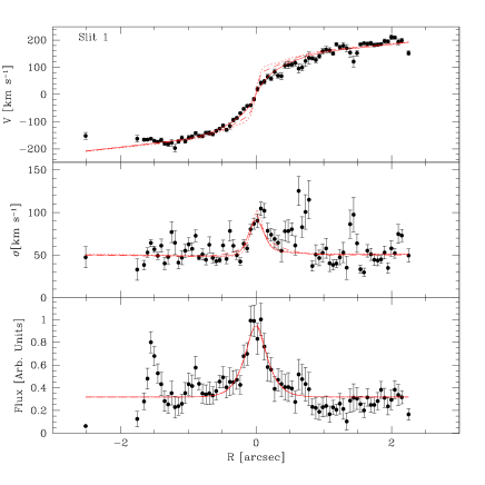
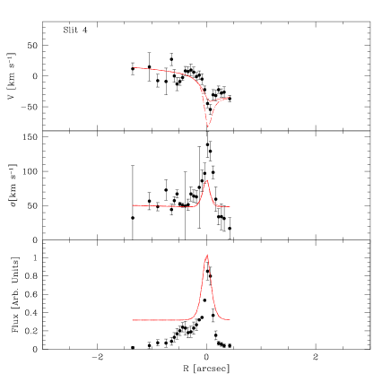
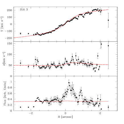
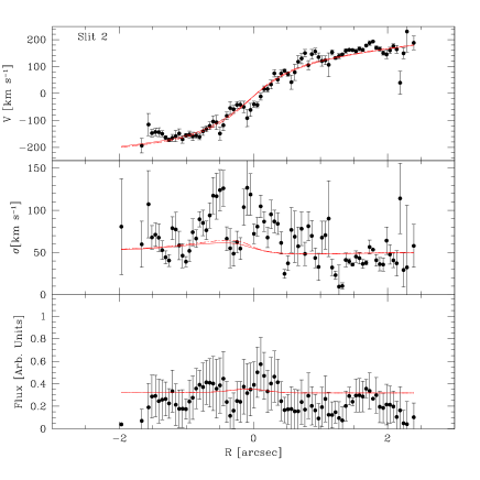
Figure 11: Observed [N II]$\,\lambda 6583$ kinematics (filled circles) along with the best-fitting model (solid line) and model predictions for the SMBH masses of NGC 4435 derived in Section 5.4 from the $M_{\bullet}$$-$$\sigma_{c}$ relation by Ferrarese & Ford (2005, $M_{\bullet}=5\cdot 10^{7}$ M_⊙, dotted line) and from the near-infrared $M_{\bullet}$$-$$L_{\it bulge}$ relation by Marconi et al. (2003, $M_{\bullet}=4\cdot 10^{7}$ M_⊙, dashed line). The observed and modeled velocity curve (top panel), velocity dispersion radial profile (middle panel) and flux radial profile (bottom panel) are shown for slit along the major axis (slit #1, upper left panels), close to minor axis (slit #4, upper right panel), along eastern offset (slit #3, lower left panel), and western offset (slit #2, lower right panel).

Finally, to account for the uncertainty in the estimate of the inclination and position angle of the gaseous disc we calculated the best-fitting values of $M_{\bullet}$ and $(M/L)_{\star}$ by building a grid of models of the gas velocity fields with $16^{\circ}\leq\theta\leq 18^{\circ}$ and $68^{\circ}\leq i\leq 72^{\circ}$. We fitted for each disc orientation the velocity dispersion and flux radial profiles measured along the major axis. The largest mass for SMBH is $M_{\bullet}$$\leq 8\cdot 10^{6}$ M_⊙ at 3$\sigma$ confidence level to find the optimized values for $F_{0}$, $F_{1}$, $r_{F}$, $\sigma_{0}$, $\sigma_{1}$, and $r_{\sigma}$. The mass-to-light ratio ranges between $(M/L)_{\star}$$=2.15^{+0.09}_{-0.12}$ and $(M/L)_{\star}$$=2.25^{+0.14}_{-0.13}$ at 3$\sigma$ confidence level. These values are consistent within the errors with the previously found values.

6 Comparison with the predictions of the near-infrared $M_{\bullet}$$-$$L_{\it bulge}$ and $M_{\bullet}$$-$$\sigma_{c}$ relations

In order to compare our SMBH mass determination for NGC 4435 with the predictions of the near-infrared $M_{\bullet}$$-$$L_{\it bulge}$ relation by Marconi & Hunt (2003), we retrieved the 2MASS $H-$band images from the NASA/IPAC Infrared Science Archive. The galaxy image was reduced and flux calibrated with the standard 2MASS extended source processor GALWORKS (Jarrett et al. 2000). We chose the $H-$band image since it is characterized by lower sky noise with respect to the $J-$ and $K-$band ones.

We performed a bidimensional photometric decomposition using a Sérsic law for the bulge component and an exponential law for the disc component and taking into account seeing smearing. We adopted the decomposition technique developed by Mendez Abreu et al. (2004). The best-fitting parameters are $n=2.39$, $r_{e}=11.14$ arcsec, $\mu_{e}=16.10$ mag arcsec^-2, and $(b/a)_{b}=0.64$ for the bulge and $h=14.41$ arcsec, $\mu_{0}=18.15$ mag arcsec^-2, and $(b/a)_{d}=0.60$ for the disc. The typical error on each parameter is $<20\%$. The total bulge luminosity is $L_{H}=2.8\cdot 10^{10}$ L_⊙, which corresponds to a $M_{\bullet}$$=4\cdot 10^{7}$ M_⊙ following Marconi & Hunt (2003). The presence of the bar in NGC 4435 is enhanced in model-subtracted image (Figure 13). However, it has to be noticed that the bar component dominates the surface-brightness distribution of NGC 4435 at a larger radial scale with respect to the extension of STIS kinematics. We conclude that the effects of the bar on the observed kinematics are negligible in the innermost 2 arcsec.

Several authors report different values for the central stellar velocity dispersion in NGC 4435.

Bernardi et al. (2002) and Tonry & Davis (1981) both reported a value of $\sigma_{c}$$=174\pm 16$ $\mathrm{km\;s}^{-1}$, whereas Simien & Prugniel (1997) measured a value of $\sigma_{c}$$=156\pm 7$ $\mathrm{km\;s}^{-1}$. The Hypercat database also lists an unpublished value of $165\pm 6$ $\mathrm{km\;s}^{-1}$ by Prugniel & Simien.

In order to be conservative, we adopted the value $\sigma_{c}$$=156\pm 7$ $\mathrm{km\;s}^{-1}$ from Simien & Prugniel (1997). Using the correction proposed by Jorgensen et al. (1995), we derived the velocity dispersion that would have been measured within a circular aperture of $1/8r_{e}$, where $r_{e}$ is the bulge effective radius derived from our photometric decomposition. We found $\sigma_{1/8}=157$ $\mathrm{km\;s}^{-1}$. According to the most recent version of the $M_{\bullet}$$-$$\sigma_{c}$ relation (Ferrarese & Ford 2005), the expected SMBH mass corresponding to this value of $\sigma_{c}$is $5\cdot 10^{7}$ M_⊙. We note that the other published values of $\sigma_{c}$would lead to even larger black-hole mass for NGC4435.

In both cases, the upper limit found in our model is significantly below the prediction of these two scaling relations. In Figure 11 we show the comparison between the observed kinematics, the best-fit model, and models adopting the prediction of the near-infrared $M_{\bullet}$$-$$L_{\it bulge}$ (Marconi & Hunt 2003) and $M_{\bullet}$$-$$\sigma_{c}$ (Ferrarese & Ford 2004) relationships, where the intrinsic velocity dispersion profiles were accordingly adjusted. The bigger discrepancies between the observed and predicted velocity fields are found in the innermost $\pm 0.25$ arcsec. In Figure 12 we report the position of the upper limit of the $M_{\bullet}$ of NGC 4435 in the $M_{\bullet}$$-$$\sigma_{c}$ and near-infrared $M_{\bullet}$$-$$L_{\it bulge}$ relations.

Figure 12: Location of the upper limit value of the SMBH mass of NGC 4435 with respect to the $M_{\bullet}$$-$$\sigma_{c}$ relation by Ferrarese & Ford (2005, left panel) and near-infrared $M_{\bullet}$$-$$L_{\it bulge}$ relation by Marconi & Hunt (2003, right panel). In the left panel, following Ferrarese & Ford (2005) we plot the SMBH masses based on resolved dynamical studies of ionised gas (open circles), water masers (open squares), and stars (filled circles). The upper limit of the SMBH mass of NGC 4335 (Verdoes Kleijn et al. 2002) has been included for sake of comparison (see Section 7). In the right panel we plot the SMBH masses which for which $H-$band luminosity of the host spheroid is available in Marconi & Hunt (2003). In both panels dotted lines represent the $1\sigma$ scatter in $M_{\bullet}$.

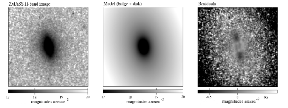
Figure 13: Two-dimensional photometric decomposition of the surface-brightness distribution of NGC 4435. Left panel: Background- and star-subtracted $H-$band image of NGC 4435 from the 2MASS archive. Central panel: Galaxy model as derived from the photometric decomposition. The bulge is modeled with a Sérsic law ($n=2.39$, $R_{e}=11\aas@@fstack{\prime\prime}14$, $\mu_{e}=16.10$ mag arcsec^-1 and $b/a=0.64$) the disc is modeled with and exponential law ($h=104\aas@@fstack{\prime\prime}41$, $\mu_{0}=18.15$ mag arcsec^-1 and $b/a=0.60$). Right panel: Residuals of the model. Images are 3 arcmin $\times$ 3 arcmin.

6.1 Uncertainties due the signal-to-noise ratio

One important point to investigate is if the $S/N$ ratio of our spectra is sufficiently high to exclude the presence of a SMBH with the mass predicted by the scaling relations. If it is not the case, the central velocity gradient is washed out by the noise and it is not possible to detect the presence of a SMBH.

To exclude this possibility we measured the noise level in the observed spectra as the rms of the counts in spectral regions free of emission lines. This noise has been added to the model spectra in order to mimic the $S/N$ ratio of the observations. Figure 14 shows that the signature of a SMBH with $M_{\bullet}$$\geq 4\cdot 10^{7}$ M_⊙ is clearly visible in the modeled major-axis spectrum which looks different than the observed one. We conclude that the velocity gradient corresponding to $M_{\bullet}$$\geq 4\cdot 10^{7}$ M_⊙ could be measured in the velocity profiles of the observed spectra.

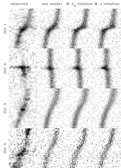
Figure 14: Comparison between the observed two-dimensional spectra (left panels) and the two-dimesional synthetic spectra for (i) the best-fitting model, (ii) a model with $M_{\bullet}$$=4\cdot 10^{7}$ M_⊙ as predicted by the near-infrared $M_{\bullet}$$-$$L_{\it bulge}$ relation, and (iii) a model with $M_{\bullet}$$=5\cdot 10^{7}$ M_⊙ as predicted by the $M_{\bullet}$$-$$\sigma_{c}$ relation for the different slit positions. In the models we added a random noise in order to mimic the actual $S/N$ ratio of the observed spectra. Each box is 15 Å $\times$ 2.6 arcsec.

6.2 Uncertainties due to the disc orientation

The upper limit we derived for $M_{\bullet}$ depends on the two assumptions we did on the orientation of the gaseous disc, i.e. the morphology of dust lanes is a good tracer of the orientation of the gaseous disc, and the gaseous disc is not warped.

We test if the presence of a SMBH with a mass of $M_{\bullet}$$=4\cdot 10^{7}$ M_⊙ (i.e., consistent with the near-infrared $M_{\bullet}$$-$$L_{\it bulge}$ relation) is consistent with the major-axis kinematics assuming for the gaseous disc a different geometrical configuration with respect to the one we derived from the dust lanes analysis. We explored the space of parameters $\theta$ and $i$ by building a grid of models of the gas velocity fields with $M_{\bullet}$$=4\cdot 10^{7}$ M_⊙ and $(M/L)_{\star}$$=2.2$. For every value of $\theta$ and $i$ we use different values of $F_{0}$, $F_{1}$, $r_{F}$, $\sigma_{0}$, $\sigma_{1}$, and $r_{\sigma}$, optimising them according to the prescription given in Section 5.4 in order to match the observations. This value is constrained by the gaseous kinematics measured in outer regions which is not influenced by the presence of the central SMBH. The best fit to the observed data is found with $i=74^{\circ}$ and $\theta=6.5^{\circ}$. Nevertheless, in the central $\pm 0.25$ arcsec there is a great discrepancy between the model and observed kinematics (Figure 15) which convinced us to reject this model as a reliable solution.

We performed also a simultaneous fit of the velocity curves leaving the parameters $M_{\bullet}$  $(M/L)_{\star}$, $\theta$ and $i$ free to vary. The best fit parameters are $M_{\bullet}$$\leq 9\cdot 10^{6}$ M_⊙, $(M/L)_{\star}$$=2.5\pm 2$ (M/L)_⊙  $\theta=15^{\circ}\pm 2^{\circ}$, and $i=75^{\circ}\pm 3^{\circ}$. Although for computational reasons this minimization is performed with all parameters for the intrinsic flux and velocity dispersion profiles fixed at the best values derived in Section 5.4, the similarity of the disc orientation found in this fit with respect to the one determined in Section 5.3 makes us confident about the choice of adopting the dust-lane morphology to constrain the orientation of the gaseous disc.

The previous results still rely on the assumption that the gas follows a coplanar distribution. However, the presence of a SMBH with a mass $M_{\bullet}$$=4\cdot 10^{7}$ M_⊙ could still be consistent with observed kinematics if the gas would warp to a more face-on orientation toward the central region. By exploring the $\theta$ and $i$ parameter space with models for the gas velocity field only within $\pm 0.25$ arcsec from the centre and with $M_{\bullet}$$=4\cdot 10^{7}$ M_⊙ and $(M/L)_{\star}$$=2.2$ (M/L)_⊙, we find that the observed kinematics could be explained if $i=28^{\circ}$ and $\theta=10^{\circ}$ (Figure 16). The images, however, do not suggest such dramatic variation of the disc orientation, and in Figure 8 in particular the dust lanes suggest an highly inclined configuration down to very small radii ($r\sim 0.5$ arcsec).

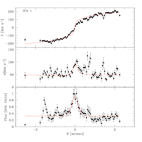
Figure 15: Observed [N II]$\,\lambda 6583$ (filled circles) and fitted (solid line) kinematics in the innermost $\pm 2.5$ arcsec along the major axis of NGC 4435 obtained with $M_{\bullet}$$=4\cdot 10^{7}$ M_⊙ and $(M/L)_{\star}$$=2.2$ (M/L)_⊙ but allowing the position angle and inclination of the gaseous disc to vary. The central velocity gradient is not reproduced by any choice of disc inclination and position angle.

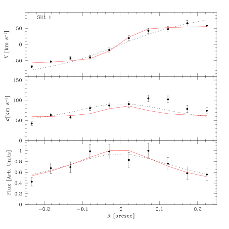
Figure 16: Observed [N II]$\,\lambda 6583$ (filled circles) and fitted (solid and dotted lines) kinematics in the innermost $\pm 2.5$ arcsec along the major axis of NGC 4435. The solid lines correspond to a model obtained with $M_{\bullet}$$=4\cdot 10^{7}$ M_⊙, $(M/L)_{\star}$$=2.2$ (M/L)_⊙, $\theta=10^{\circ}$ and $i=28^{\circ}$ in the innermost $\pm 2.5$ arcsec. The dashed lines correspond to a model obtained with $M_{\bullet}$$=0$ M_⊙, $(M/L)_{\star}$$=2.2$ (M/L)_⊙, $\theta=17^{\circ}$ and $i=70^{\circ}$.

6.3 Uncertainties due to the slit position

The upper limit we derived depends also on the assumed position of the slits. In Section 3.3 we determined the actual position of the slits by comparing the light profile of the spectrum with the light profiles extracted from the acquisition image. In the case that this procedure is not reliable, we try to find new slits position (but not changing their relative distance) in order to allow the presence of a $M_{\bullet}$$=4\cdot 10^{7}$ M_⊙. We used the parameters $\theta=17^{\circ}$ and $i=70^{\circ}$ and $(M/L)_{\star}$$=2.2$ (M/L)_⊙ and we find that the major axis velocity gradient is well reproduced if we shift the slit of 3 STIS pixels. But in that case, the kinematics along the parallel offset slits is not reproduced anymore: there are no ways to reproduce simultaneously all the slits. Having parallell slits provide a kinematic test for correct slit positioning, which confirmed the slit locations inferred in Section 3.3, using the acquisition images.

6.4 Effects of the flux distribution on the measurements

Without narrow-band images we had to resort an analytical description for the intrinsic surface brightness of the ionised gas (see Section 5.1.2). Our choice of an exponential radial profile for the emission-line fluxes seems well-justified a posteriori given the good match to observed flux profiles along all slit positions, particularly towards the centre (see Figure 11). However, as in the case of NGC 3245 (Barth et al. 2001), it is likely that unaccounted small-scale flux fluctuations are responsible for the poor match in many part of the velocity curve (see Section 5.4)

As far as the SMBH mass measurement is concerned, it is important to bear in mind our ignorance of the details characterising the gas surface brightness towards the very centre of the NGC 4435. In particular, the presence of nuclear dust may represent a limitation for our analysis. If the very central regions, where the gas clouds are more directly affected by the gravitational pull of the SMBH, are affected by significant dust absorption, it possible that gas further away from the centre and moving at slower speed could contribute to the observed central velocity gradient and flux peak. If this is the case we would be underestimating the SMBH mass.

We investigated this possibility by using a different model for the intrinsic gas surface-brightness, including an additional central component with negative amplitude, to mimic a central flux depletion due to dust absorption. We have started by trying to accomodate a $4\cdot 10^{7}$ M_⊙ SMBH. As shown by Figure 17, to match the observed gas rotation significant dust absorption is required out to about 1 arcsec, but in this case the predicted flux distribution is inconsistent with the observed profile. The extent of the nuclear dust is a direct consequence of the fact that the observed rotation curve can be fitted without a SMBH (Figure 11), so that dust have to screen the emission from regions where the SMBH can contribute significantly to the observed rotation curve. For a $(M/L)_{\star}$= 2.2, including a $4\cdot 10^{7}$ M_⊙ SMBH still increases the circular velocity (Eq. 1) by 10 $\mathrm{km\;s}^{-1}$ at a radius of 55 pc, corresponding to $0.7$ arcsec.

In this framework, to explain the observed flux profile we would need to resort to fine-tuned geometries for the gas distribution in which intervening off-plane material would contribute to the observed central peak in flux distribution. However, the exceptional regularity of the dust distribution in our images and the well-established connection between dust and gas (e.g., Pogge et al. 2000) strongly suggest that the gas resides on a simple a simple disc.

Furthermore, the required amount of central flux depletion needed to accomodate a $4\cdot 10^{7}$ M_⊙ SMBH would translate into an additional central reddening of $E(B-I)=1.3$ mag. which is should be easily detected in our map for the $E(B-I)$ color excess (Figure 5, in which the central value is $0.6$ mag.). This is not the case, however. In this calculation we had taken into account i) the different value of the extinction $A_{\lambda}$ at different wavelenght (the $I-$band and the [N II]$\,\lambda 6583$ region , using the standard Galactic extinction as done in Cardelli et al. 1989); ii) that only the light from stars behind the dusty disc is absorbed.

We therefore consider it unlikely that nuclear dust could hide a SMBH consistent with the expectations of the $M_{\bullet}$$-$$\sigma_{c}$ relation. On the other hand, it is still possible that nuclear dust could impact our inferred upper limit on the SMBH mass while still matching the flux profile. In this case however, the central dust cannot extend beyond the width of our slit. The impact on $M_{\bullet}$ will therefore be rather limited; we find that our upper limit would increase by only few percent, to $8\cdot 10^{6}$ M_⊙. Gaussian profile instead of an exponential profile for the flux distribution, as done by Sarzi et al. (2001, 2002), would have a similar small effect.

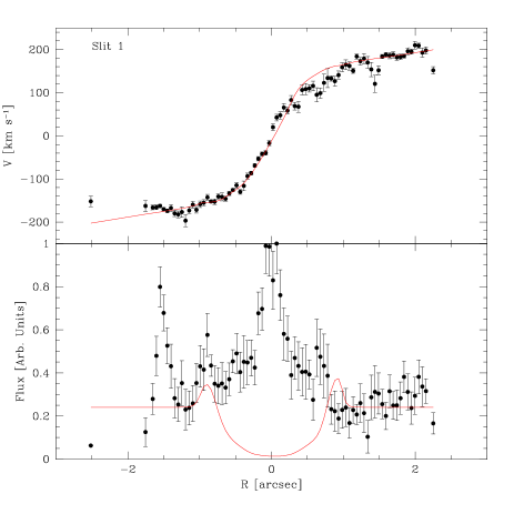
Figure 17: Observed [N II]$\,\lambda 6583$ (filled circles) and fitted (solid lines) kinematics in the innermost $\pm 2.5$ arcsec along the major axis of NGC 4435. The model is obtained using a $M_{\bullet}$=$4\cdot 10^{7}$ M_⊙ $i=70^{\circ}$, $\theta=17^{\circ}$, $(M/L)_{\star}$$=2.2$ (M/L)_⊙, and an ad hoc flux distribution to reproduce the central gradient. The predicted flux radial profile is completely inconsistent with the observed one.

6.5 Correction for asymmetric drift

The velocity dispersion of the gas peaks at 100 $\mathrm{km\;s}^{-1}$ in the centre. This intrinsic line width is far higher than that expected either from rotational and instrumental broadening or from thermal motion. This finding is in agreement with earlier results on bulges of other disc galaxies based on both ground-based (Fillmore et al. 1986; Bertola et al. 1995; Cinzano et al. 1999; Pignatelli et al. 2001) and STIS spectroscopy (Barth et al. 2001) and suggests that random motions may be crucial for the dynamical support of the gas. If ionised-gas disc is fragmented into collisionless clouds, then dynamical pressure supports it against gravity and the mean rotational velocity $v_{\phi}$ is smaller than the circular velocity $v_{c}$ given in Equation 1. As a consequence, the enclosed mass is underestimated by dynamical models which do not account for the asymmetric drift correction.

In the following we address how much of an effect this would have on the difference between the velocity gradient we measured and that we inferred for gas rotating around a SMBH with $M_{\bullet}$$=4\cdot 10^{7}$ M_⊙ as predicted by the near-infrared $M_{\bullet}$$-$$L_{\it bulge}$ scaling relation.

We assume that the motions in the gas disc are close to isotropic in the radial and vertical direction. Then $\sigma_{z}=\sigma_{r}$ and $\left<v_{r}v_{z}\right>=0$, and the asymmetric drift correction can be expressed as

$$v_{c}^{2}-v_{\phi}^{2}=\sigma_{r}^{2}\left[-r\frac{d\ln\nu}{dr}-r\frac{d\ln\sigma_{r}^{2}}{dr}-\left(1-\frac{\sigma_{r}^{2}}{\sigma_{\phi}^{2}}\right)\right]$$ (12)

where $\sigma_{\phi}$ is the azimuthal velocity dispersion and $\nu$ is the number density of gas clouds in the disc (e.g., Binney & Tremaine 1987). We assume that the number density of the gas clouds is proportional to the gas flux whose radial profile has been parametrized in Eq. 3. The relation between $\sigma_{r}$ and $\sigma_{\phi}$ is given by the epicycle approximation

$$\frac{\sigma_{\phi}^{2}}{\sigma_{r}^{2}}=\frac{-B}{A-B}$$ (13)

where $A$ and $B$ are the Oort constants given by

$$A = \frac{1}{2}\left(\frac{v_{c}}{r}-\frac{dv_{c}}{dr}\right)$$ (14)

$$B = -\frac{1}{2}\left(\frac{v_{c}}{r}+\frac{dv_{c}}{dr}\right).$$ (15)

The approximation is strictly valid in the limit $\sigma\ll v_{c}$. If we assume that the SMBH mass is given by the near-infrared $M_{\bullet}$$-$$L_{\it bulge}$ relation, we have a ratio $\sigma_{r}/v_{c}<0.32$ everywhere in the gaseous disc of NGC 4435 (Figure 18) and the method can be adopted for at least an approximate treatment of the asymmetric drift. After calculating the asymmetric drift, we obtained the line-of-sight velocity and velocity dispersion as

$$v=v_{\phi}\left(\frac{y\sin{i}}{r}\right)$$ (16)

and

$$\sigma=(\sigma_{\phi}^{2}-\sigma_{r}^{2})\left(\frac{y\sin{i}}{r}\right)^{2}+\sigma_{r}^{2},$$ (17)

respectively. These values of $v$ and $\sigma$ are used in Eq. 9 for the model calculation. For models without an asymmetric drift, the above equations reduce to $v_{c}=v_{\phi}$ and $\sigma=\sigma_{r}=\sigma_{\phi}$, corresponding to the case where the intrinsic velocity dispersion represents a locally isotropic turbulence within the gaseous disc.

We applied the asymmetric drift correction for $M_{\bullet}$$=4\cdot 10^{7}$ M_⊙ and found that the contribution of intrinsic velocity dispersion to the rotation curve is negligible ($\leq 5\%$). The comparison between the model rotation curves obtained along the galaxy major axis with and without the asymmetric drift correction is shown in Figure 19. We can conclude that the contribution of the velocity dispersion is not enough to allow the presence of $M_{\bullet}$$=4\cdot 10^{7}$ M_⊙ in the nucleus of NGC 4435.

Figure 18: The ratio $\sigma_{r}/v_{c}$ for the model with $M_{\bullet}$$=4\cdot 10^{7}$ M_⊙.

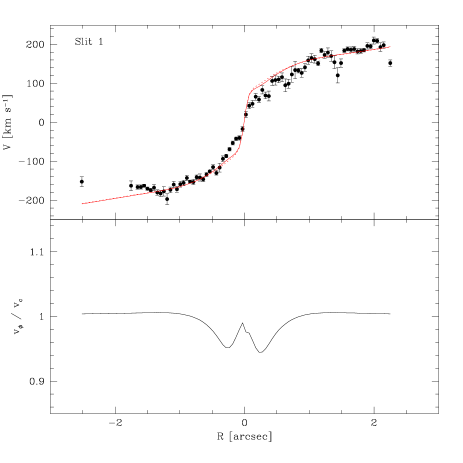
Figure 19: Upper panel: The observed [N II]$\,\lambda 6583$ (filled circles) along the the major axis of NGC 4435 is compared to the one obtained with $M_{\bullet}$$=4\cdot 10^{7}$ M_⊙, $(M/L)_{\star}$$=2.2$ (M/L)_⊙, $\theta=17^{\circ}$ and $i=70^{\circ}$ with (solid line) and without (dashed line) applying the asymmetric drift correction. Lower panel: Ratio between the rotation curves obtained with and without applying the asymmetric drift correction.

7 Conclusions

We presented long-slit STIS measurements of the ionised-gas kinematics in the nucleus of the SB0 NGC 4435. NGC 4435 belongs to a sample of 3 galaxies which were selected as STIS targets on the basis of their CNKD kinematics (Bertola et al. 1998).

For NGC 4435 we found the following:

(i) It shows a CNKD with a symmetric and regular ionised-gas kinematics, which is suitable for dynamical modeling in order to estimate the mass of the central SMBH. Moreover, NGC 4435 is characterized by the presence of smooth and circularly symmetric dust lanes. This result is in agreement with early findings of Ho et al. (2002) who found an empirical correlation between the morphology of the dust lanes and the degree of regularity in the gas velocity field.

Bertola et al. (1998) demonstrated that it is possible to detect the signature of a CNKD in the emission-line PVDs obtained from ground-based spectroscopy of nearby galaxies. Using this result, Funes et al. (2002) estimated that the frequency of CNKDs in randomly selected emission-line disc galaxies is $\la 20\%$. However, this criterion has to be combined with that of the presence of a regular dust-lane morphology (Ho et al. 2002). On the basis of our STIS observations, we conclude that less than $10\%$ of nearby disc galaxies, which show narrow emission lines in their ground-based spectra, host a CNKD with a velocity field which is useful for dynamical modeling at HST resolution.

(ii) We modeled the ionised-gas velocity field of NGC 4435 by assuming the gas is moving onto circular orbits in an infinitesimally thin disc located around the SMBH. We constrained the orientation of the gaseous disc ($\theta=17^{\circ}\pm 1^{\circ}$, $i=70^{\circ}\pm 2^{\circ}$) by assuming that the morphology of dust lanes is tracing the gas distribution. The comparison between the observed and modeled velocity field has been done by taking into account several effects related to telescope and instrument optics (nonzero aperture size, apparent wavelength shifts for light entering the slit off centre, and anamorphic magnification) as well as detector readout (charge bleeding between adjacent CCD pixels). We derived for the SMBH mass of NGC 4435 an upper limit $M_{\bullet}\leq 7.5\cdot 10^{6}$ M_⊙ at 3$\sigma$ confidence level.

(iii) The upper limit we derived for the SMBH mass of NGC 4435 considerably falls short of the value of $M_{\bullet}$$=4\cdot 10^{7}$ M_⊙ predicted by the $M_{\bullet}$$-$$\sigma_{c}$ relation (Ferrarese & Ford 2005), as well as of the value of $M_{\bullet}$$=5\cdot 10^{7}$ M_⊙ predicted by the near-infrared $M_{\bullet}$$-$$L_{\it bulge}$ relation (Marconi & Hunt 2003) as shown in Figure 12. This discrepancy is not due to the noise in our spectra (Section 6.1), is robust against uncertainties in the disc orientation (Section 6.2) or slit positioning (Section 6.3), and cannot be ascribed to the presence of nuclear dust (Section 6.4) or pressure-supported gas (Section 6.5). The measured velocity gradient is consistent with a $M_{\bullet}$$=4\cdot 10^{7}$ M_⊙ only if we assume an ad hoc orientation ($\theta=10^{\circ}\pm 1^{\circ}$, $i=28^{\circ}\pm 2^{\circ}$) for the central portion of the gaseous disc ($|r|\leq 0.25$ arcsec). However, the images do not suggest such a dramatic variation of the disc orientation in the observed radial range.

(iv) The case of NGC 4435 is very similar to that of the elliptical NGC 4335 (Verdoes Kleijn et al. 2002), where the ionised-gas kinematics measured with STIS along three parallel positions is consistent with that of a CNKD rotating around a SMBH with an unusually low mass ($M_{\bullet}\leq 10^{8}$ M_⊙) for its high velocity dispersion ($\sigma_{c}$$=300\pm 25$ $\mathrm{km\;s}^{-1}$, see Figure 12). Both NGC 4435 and NGC 4335 are amenable to gas dynamical modeling. Their nuclear discs of ionised gas have a well-constrained orientation as well as a symmetric and regular velocity field. There is no evidence that gas is affected by non-gravitational motions or that it is not in equilibrium, as observed for instance in the E3 galaxy IC 1459 (Cappellari et al. 2002) and the Sbc NGC 4041 (Marconi et al. 2003). For NGC 4335 the observed high gas velocity dispersion in the central arcsec potentially invalidates the $M_{\bullet}$ measurement based on a thin rotating disc model leading to a larger $M_{\bullet}$ value and to a smaller discrepancy with the $M_{\bullet}$ scaling laws. On the contrary, in NGC 4435 the more limited width of the lines allowed us to consider the possibility of a modest dynamical support for the gas clouds. This has little impact on the measured $M_{\bullet}$ and can not explain its discrepancy with the values predicted by the $M_{\bullet}$ scaling relations. As such, if we suppose the resulting upper limit for the SMBH mass of NGC 4435 is also unreliable, we are then forced to conclude that all the SMBH masses derived from gaseous kinematics following standard assumptions have to be treated with caution, even if they agree with the predictions of the scaling relations.

Thus, NGC 4435 is so far the best candidate of a galaxy with a massive bulge component with a lower $M_{\bullet}$ content than predicted by the $M_{\bullet}$$-$$\sigma_{c}$ and $M_{\bullet}$$-$$L_{\it bulge}$ scaling relations. Nevertheless, there is an increasing evidence of galaxies for which dynamical models impose an upper limit to the SMBH mass which is either lower than or marginally consistent with the one predicted by the $M_{\bullet}$$-$$\sigma_{c}$ (Sarzi et al. 2001; Merritt et al. 2001; Gebhardt et al. 2001; Valluri et al. 2005). These objects may represent the population of laggard SMBHs with masses below the $M_{\bullet}$$-$$\sigma_{c}$ relation as discussed by Vittorini et al. (2005). Laggard SMBHs are expected to reside in galaxies that spent most of their lifetime in the field, where encounters are late and rare so as to cause only slow gas fueling of the galactic centre and a limited growth of the SMBH mass.

In light of the serious implications on the slope and intrinsic scatter of the $M_{\bullet}$ relations that our results would imply, an independent measurement of the SMBH mass NGC 4435 based on stellar dynamical modeling is highly desirable. This could be done with near-infrared spectroscopic observations with 8m-class telescopes assisted by adaptive optics systems. Recently, Houghton et al. (2005) have shown in the case of the giant elliptical NGC 1399 that this technique can deliver diffraction limited high signal-to-noise spectra suitable for measuring the stellar LOSVD within the sphere-of-influence of the SMBH, providing a concrete alternative to HST that today is in serious jeopardy.

Acknowledgements.

EDB acknowledges the Fondazione “Ing. Aldo Gini” for a research fellowship, and the Herzberg Institute of Astrophysics, Victoria, BC, for the hospitality while this paper was in progress. We wish to thank Aaron Barth and Laura Ferrarese for stimulating discussions, Alfonso Cavaliere and Valerio Vittorini for providing us their results about laggard SMBHs prior to publication. We are indebted to Jairo Mendez Abreu for the package which we used for measuring the photometric parameters of NGC 4435. This research has made use of the Lyon-Meudon Extragalactic Database (LEDA) and of the NASA/IPAC Extragalactic Database (NED). We would like to thank the anonymous referee for constructive comments.

Appendix A Calculation of the color excess $E(B-I)$ in the case of a $M_{\bullet}$$=4\cdot 10^{7}$ M_⊙

In this section we evaluate the colour excess $E^{\prime}(B-I)$ we would expect in the case that a $M_{\bullet}$$=4\cdot 10^{7}$ M_⊙ is present and the absorption of the central dust is able to reproduce the observed kinematics (see Section 6.4).

If the ionised gas is settled in the equatorial plane as well as the dust, the intrinsic flux corrected by absorption ($F^{abs}$) will be related to the intrinsic one ($F^{ems}$) by the relation

$$F^{abs}=10^{-0.4A_{[NII]}}\cdot F^{ems}=(1-c)\cdot F^{ems}$$ (18)

The coefficient $c$ indicates the efficiency of the absorption, and it can be easily derived (see Figure 20). For $c=1$, $F^{abs}=0$, for $c=0$, $F^{abs}=F^{ems}$.

Using the standard Galactic extinction (Cardelli et al. 1989) we can determine the relation between the extinction $A_{[NII]}$ and the extinction in the I band, $A_{I}$:

$$A_{I}=0.588A_{[NII]}$$ (19)

The central stellar component (bulge plus disc) is thicker with respect the ionised gas and the dust discs. Thus, only the portion of stars behind the dust layer is absorbed:

$$F_{star}^{abs}=\frac{1}{2}F_{star}^{ems}+\frac{1}{2}10^{-0.4\cdot A_{I}}F_{star}^{ems}=\frac{1+10^{-0.4\cdot A_{I}}}{2}F_{star}^{ems}$$ (20)

What we should observe is the extinction $A^{\prime}_{I}$ defined by:

$$F_{star}^{abs}=10^{-0.4\cdot A^{\prime}_{I}}\cdot F_{star}^{ems}$$ (21)

with (comparing Eqs. A3 and A4):

$$A^{\prime}_{I}=-2.5\log\frac{1+10^{-0.4\cdot A_{I}}}{2}$$ (22)

Then, according to the standard Galactic extinction (Cardelli et al. 1989), the expected color excess $E^{\prime}(B-I)$ is:

$$E^{\prime}(B-I)=A^{\prime}_{I}/0.5583$$ (23)

Then, combining Eqs. A1, A2, A5 and A6, it is possible to calculate the map of $E^{\prime}(B-I)$ as a function of $c$, derived from Figure 20.

$$E^{\prime}(B-I)=-4.48\log\frac{1+(1-c)^{0.588}}{2}$$ (24)

In the central region, where $c=1$ the expected color excess is 1.3 mag, while the observed one is 0.6 mag. (Figure 5).

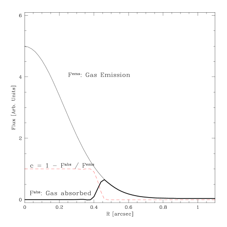
Figure 20: Intrinsic flux radial profile of the gas in the NGC 4435 model. The solid thin line shows the intrinsic emission of our best model, whereas the solid thick line shows the absorbed emission needed to accomodate a $M_{\bullet}$$=4\cdot 10^{7}$ M_⊙ and match the observed velocities (Figure 17). The dashed line shows the efficiency of the dust absorption, $c$, as defined in the text.

References

- [xxx] Baes, M., Buyle, P., Hau, G. K. T., & Dejonghe, H., 2003, MNRAS, 341, L44
- [xxx] Barth, A. J. 2004, in Coevolution of Black Holes & Galaxies, ed. L. C. Ho (Cambridge: Cambridge Univ. Press), 21
- [xxx] Barth, A. J., Sarzi, M., Rix, H,-W, Ho, L. C., Filippenko, A. V.,& Sargent, W. L. W. 2001, ApJ, 555, 685
- [xxx] Bernardi, M., Alonso, M. V., da Costa, L. N., et al. 2002, AJ, 123, 2990
- [xxx] Bertola, F., Cinzano, P., Corsini, E. M., Rix, H.-W., & Zeilinger, W. W. 1995, ApJ, 448, L13
- [xxx] Bertola, F., Cappellari, M., Funes, J. G., Corsini, E. M., Pizzella, A., & Vega Beltrán, J. C. 1998, ApJ, 509, L93
- [xxx] Binney, J., & Tremaine, S. 1994, Galactic Dynamics (Princeton University Press: Princeton)
- [xxx] Bowers, C., & Baum, S. 1998, STIS Instrument Science Rep. 98-23 (Baltimore: STScI)
- [xxx] Brown, T. et al. 2002, in HST STIS Data Handbook, version 4.0, ed. B. Mobasher, Baltimore, STScI
- [xxx] Cappellari, M., et al. 2002, ApJ, 578, 787
- [xxx] Cardelli, J. A., Clayton, G. C., & Mathis, J. S. 1989, ApJ, 345, 245
- [xxx] Cinzano, P., Rix, H.-W., Sarzi, M., Corsini, E. M., Zeilinger, W. W., & Bertola, F. 1999, MNRAS, 307, 433
- [xxx] de Vaucouleurs, G., de Vaucouleurs, A., Corwin, H. G. Jr., Buta, R. J., Paturel, G., & Fouquè, P. 1991, Third Reference Catalogue of Bright Galaxies (New York: Springer-Verlag) (RC3)
- [xxx] Ferrarese, L., 2002, ApJ, 578, 90
- [xxx] Ferrarese, L., & Merritt, D., 2000, ApJ, 539, L9
- [xxx] Ferrarese, L., & Ford, H. 2005, Space Science Reviews, 116, 523
- [xxx] Fillmore, J. A., Boroson, T. A., & Dressler, A. 1986, ApJ, 302, 208
- [xxx] Funes, J. G., S. J, Corsini, E. M., Cappellari, M., Pizzella, A., Vega Beltrán, J. C., Scarlata, C., & Bertola, F. 2002, A&A, 388, 50
- [xxx] Gebhardt K., et al., 2000, ApJ, 539, 13
- [xxx] Gebhardt K., et al., 2001, AJ, 122, 2469
- [xxx] Ghez, A.M., et al. 2003, ApJ, 586, L127
- [xxx] Graham, J. A., Ferrarese, L., Freedman, W. L., et al. 1999, ApJ, 516, 626
- [xxx] Graham, A. W., Erwin, P., Caon, N., & Trujillo, I. 2001, ApJ, 563, L11
- [xxx] Guthrie, B. N. G. 1992, A&AS, 93, 255
- [xxx] Häring, N., & Rix, H.-W. 2004, ApJ, 604, L89
- [xxx] Ho, L. C., et al. 2002, PASP, 114, 137
- [xxx] Holtzman, J. A., Burrows, C. J., Casertano, S., Hester, J. J., Trauger, J. T., Watson, A. M., & Worthey, G. 1995, PASP, 107, 1065
- [xxx] Houghton, R. C. W., Magorrian, J., Sarzi, et al. 2005, MNRAS in press (astro-ph/0510278)
- [xxx] Jarrett, T. H., Chester, T., Cutri, R., Schneider, S., Skrutskie, M., & Huchra, J. P. 2000, AJ, 119, 2498
- [xxx] Jorgensen, I., Franx, M., & Kjaergaard, P., 1995, MNRAS, 276, 1341
- [xxx] Kinney, A. L., Calzetti, D., Bohlin, R. C., McQuade, K., Storchi-Bergmann, T., & Schmitt, H. R. 1996, ApJ, 467, 38
- [xxx] Kormendy, 2001, Rev. Mexicana Astron. Astrofis, Ser. Conf., 10, 69
- [xxx] Kormendy, J. 2004, in Coevolution of Black Holes & Galaxies, ed. L. C. Ho (Cambridge: Cambridge Univ. Press), 1
- [xxx] Kormendy, J. & Richstone, D. 1995, ARA&A, 33, 581
- [xxx] Krist, J., & Hook, R. 1999, The Tiny Tim User’s Guide (Baltimore: STScI)
- [xxx] Maciejewski, W.,& Binney, J. 2001, MNRAS, 323, 831
- [xxx] Magorrian, J., et al. 1998, AJ, 115, 2285
- [xxx] Marconi, A., & Hunt, L. K. 2003, ApJ, 589, 21
- [xxx] Marconi, A., et al. 2003, ApJ, 586, 868
- [xxx] Mendez Abreu, J., Corsini, E. M., Aguerri, J. A. L. 2004, in Baryons in Dark Matter Halos, ed. R. Dettmar, U. Klein, & P. Salucci, PoS (Trieste: SISSA), p.83.1
- [xxx] Merritt D., Ferrarese L., Joseph C. L., 2001, Sci, 293, 1116
- [xxx] Miyoshi, M., Moran, J., Herrnstein, J., Greenhill, L., Nakai, N., Diamond, P., & Inoue, M. 1995, Nature, 373, 127
- [xxx] Monnet, G., Bacon, R., & Emsellem, E. 1992, A&A, 253, 366
- [xxx] Pignatelli, E., Corsini, E. M., Vega Béltran, J. C., Scarlata, C., et al. 2001, MNRAS, 320, 124
- [xxx] Pizzella, A., Corsini, E. M., Morelli, L., Sarzi, M., Scarlata, C., Stiavelli, M., & Bertola, F. 2002, ApJ, 573, 131
- [xxx] Pizzella, A., Corsini, E. M., Dalla Bontà, E., Sarzi M., Coccato, L., & Bertola, F. 2005, ApJ, 631, 785
- [xxx] Pogge, R. W., Maoz, D., Ho, L. C., & Eracleous, M. 2000, ApJ, 532, 323
- [xxx] Press, W. H., Teukolsky, S. A., Vetterling, W. T., & Flannery, B. P. 1992, Numerical Recipes in Fortran 77 (2d ed.: Cambridge: Cambridge University Press)
- [xxx] Rubin, V. C., Kenney, J. D. P., & Young, J. S. 1997, AJ, 113, 1250
- [xxx] Sarzi, M., et al. 2001, ApJ, 550, 65
- [xxx] Simien, F., & Prugniel, Ph. 1997, A&AS, 126, 15
- [xxx] Sofue, Y., Tomita, A., Tutui, Y. Honma, M.,& Takeda, Y. 1998, PASJ, 50, 427
- [xxx] Tonry, J.& Davis, M. 1981, ApJ, 246, 666
- [xxx] Valluri, M., Ferrarese, L., Merritt D., Joseph C. L., 2005, ApJ, 628, 137
- [xxx] van Dokkum, P. G. 2001, PASP, 113, 1420
- [xxx] Verdoes Kleijn, G. A., van der Marel, R. P., de Zeeuw, P. T., Noel-Storr, J., Baum, S. A. 2002, AJ, 124, 2524
- [xxx] Vittorini, V., Shankar, F.,& Cavaliere, A. 2005, MNRAS, in press (astro-ph/0508640)
- [xxx] Whitmore, B. 1995, in Calibrating Hubble Space Telescope: Post Servicing Mission, ed. A. Koratkar & C. Leitherer (Baltimore: STScI), 269