REVERBERATION MEASUREMENTS OF THE INNER RADIUS OF THE DUST TORUS IN NEARBY SEYFERT 1 GALAXIES

Abstract

The most intense monitoring observations yet made in the optical ($UBV$) and near-infrared ($JHK$) wave bands were carried out for several well-known nearby Seyfert 1 galaxies of NGC 5548, NGC 4051, NGC 3227, and NGC 7469. Over three years of observations, after the operation of the MAGNUM telescope started in early 2001, clear time-delayed response of the $K$-band flux variations to the $V$-band flux variations was detected for all of these galaxies. Their $H-K$ color temperature was estimated to be $1500-1800$ K from the observed flux variation gradients. This estimated $H-K$ color, along with the smoothness of the flux variation in the near-infrared in contrast with rapid fluctuations in the optical, supports a view that the bulk of the $K$ flux should originate in the thermal radiation of hot dust that surrounds the central engine. Cross-correlation analysis was performed in order to quantify the lag time corresponding to the light-travel distance of the hot dust region from the central engine. The measured lag time is $47-53$ days for NGC 5548, $11-18$ days for NGC 4051, about $20$ days for NGC 3227, and $65-87$ days for NGC 7469. We found that the lag time is tightly correlated with the optical luminosity as expected from dust reverberation ($\Delta t\propto L^{0.5}$), while only weakly with the central virial mass, which suggests that an inner radius of the dust torus around the active nucleus has a one-to-one correspondence to central luminosity. In the lag time versus central luminosity diagram, the $K$-band lag times place an upper boundary on the similar lag times of broad-emission lines in the literature. This not only supports the unified scheme of AGNs, but also implies a physical transition from the BLR out to the dust torus that encircles the BLR. Furthermore, our $V$-band flux variations of NGC 5548 on timescales of up to 10 days are found to correlate with X-ray variations and delay behind them by one or two days, indicating the thermal reprocessing of X-ray emission by the central accretion flow.

1 INTRODUCTION

The unified scheme of active galactic nuclei (AGNs) and radio-quiet quasars explains that Seyfert 1 nuclei with broad emission-line regions (BLR) would be classified as Seyfert 2 if high velocity clouds emitting broad emission lines were hidden by the dust tori that encircle such clouds (Antonucci 1993). Outside the dust torus there would be a narrow emission-line region (NLR) that extends to more than kilo-parsecs and is often observed as resolved images. However, the angular scale of the inner dust torus even in the nearest AGN is too small to be spatially resolved with any current technology in optical and near-infrared imaging observations.

It is generally accepted that the near-infrared emission from Seyfert galaxies and quasars is thermally produced by hot dust heated by UV radiation from the central engine. Barvainis (1987, 1992) developed a dust-emission model that naturally explains the bump or excess in the near-infrared continuum of AGNs by thermal emission from grains at their sublimation temperature in a range of $1300-2000$ K. This model, which is supported by the fact that a variety of AGNs have blackbody components of nearly uniform temperature of $\sim 1500$ K (Kobayashi et al. 1993), necessarily claims a dust distribution with central hole. A typical UV luminosity of $10^{42}-10^{44}$ ergs s^-1 for Seyfert galaxies therefore gives an inner radius of $0.01-0.1$ pc or $10-100$ light days at which hot dust sublimates. Consequently, if we monitor their continuum fluxes in the UV/optical and near-infrared, a lag time would be expected that corresponds to the light-travel distance between the central engine and the hot dust region from which the bulk of near-infrared emission radiates (e.g., Clavel, Wamsteker & Glass 1989; Nelson 1996; Glass 2004).

The most successful similar technique is the reverberation mapping of the BLR carried out for many Seyfert 1 galaxies and quasars during the last decade (e.g., Peterson 1993; Wandel, Peterson & Malkan 1999; Kaspi et al. 2000). If we verify that the infrared lag is longer than the lag of broad emission lines of lower ionization energy, the inner radius of the dust torus should be larger than the outer extension of the BLR, which provides strong support to the unified scheme of AGNs. However, there have only been a few cases where lag times for both BLR and dust torus were measured for the same AGN (Clavel, Wamstekar & Glass 1989; Minezaki et al. 2004; Suganuma et al. 2004), mostly because long-term simultaneous monitoring observations in the UV/optical and near-infrared for dust reverberation have rarely been attempted.

The MAGNUM (Multicolor Active Galactic Nuclei Monitoring) project was proposed to carry out such monitoring observations for many AGNs (Kobayashi et al. 1998a; Yoshii 2002). This project built a new 2-m optical-infrared telescope at the University of Hawaii’s Haleakala Observatory on the Hawaiian island of Maui, and started preliminary observations in early 2001. Light curve data of high photometric accuracy and frequent sampling have been accumulating since then.

This paper reports early results for four nearby Seyfert 1 galaxies included in the MAGNUM program, including NGC 5548, NGC 4051, NGC 3227, and NGC 7469 for which the extent of the BLR and the central virial mass were previously derived from reverberation mapping of the BLR. The intensive monitoring observations using the MAGNUM telescope, with an improved technique for calculation of cross-correlation functions, enable the most accurate measurement of lag times between the $V$ and $K$ flux variations for the above four galaxies, and comparison with lag times for the broad emission lines.

In §2 we describe the target AGNs, the observational conditions, the image reduction, and photometry procedures. In §3 we discuss the characteristics of multicolor light curves of the target AGNs and their optical to near-infrared colors. We interpret the clear lag between optical and near-infrared variations in terms of dust reverberation. In §4 we perform a cross-correlation analysis to quantify the lag time between the $V$ and $K$ flux variations. Here, we describe how to calculate the cross-correlation functions based on two methods optimized for our time series data. In §5 we discuss how well the measured lag times for the target AGNs relate to their optical nuclear luminosities and central masses, in combination with our earlier result of NGC 4151 (Minezaki et al. 2004) and previous lag time measurements for other AGNs in the literature. We compare these lag times with similar lag-time measurements for the broad emission lines, in order to see how the inner edge of the dust torus relates to the BLR.

2 OBSERVATION AND DATA REDUCTION

2.1 Observation

The characteristics of the target AGNs (NGC 5548, NGC 4051, NGC 3227, and NGC 7469) are listed in Table 1. All of them are classified as Seyfert 1 galaxies. The right ascension and declination for an epoch of 2000 are given in columns 2 and 3, respectively. The apparent magnitude of average nuclear flux is given in column 4. The recession velocity and the Galactic $V$-band extinction are given in columns 5 and 6, respectively, from the NED database. Assuming a Hubble constant of $H_{0}=70$ km s^-1Mpc^-1, the absolute $V$ magnitude estimated from column 4 is given in column 7, after being corrected for Galactic extinction in column 6, based on the average fluxes given in the next section (Table 7).

The light curve data have been accumulated over the last several years, since the MAGNUM observatory started its operation in early 2001. A part of the early result has already been published as letters (NGC 4151, Minezaki et al. 2004; NGC 5548, Suganuma et al. 2004).

Monitoring observations were made using the multi-color imaging photometer (MIP) mounted on the MAGNUM telescope (Kobayashi et al. 1998a,b). The field of view of the MIP is 1.5 $\times$ 1.5 arcmin², and it enables us to obtain the images simultaneously in the optical and the near-infrared bands by splitting the incident beam into two different detectors such as an SITe CCD (1024 $\times$ 1024 pixels, 0.277 arcsec/pixel) and an SBRC InSb array (256 $\times$ 256 pixels, 0.346 arcsec/pixel).

Monitoring observations in the $V$ and $K$ bands started in 2001, NGC 4051 in January, NGC 5548 in March, NGC 7469 in June, and NGC 3227 in November, while the $UBJH$ observations started later. The nuclear fluxes with the $V$ and $K$ filters were observed as the first priority, and the sampling interval for each target AGN was set shorter than one tenth of the expected lag time between the $V$ and $K$ flux variations. The $B$ and $H$ filters were used as the second priority, and the $U$ and $J$ filters as the third priority.

The telescope was pointed, typically six times, at each of the target AGN and two reference stars A and B, alternately. The pointings were repeated first in order of A $\rightarrow$ AGN $\rightarrow$ B, then in the reverse order with small shift of several arcsecs, and so on, which gave us dithered field images of the AGN and the stars. In each pointing, the CCD detector was exposed at once during which the InSb array was read out several times or more to avoid saturation. High signal-to-noise ratios were achieved with total on-source integration time of several minutes for each object.

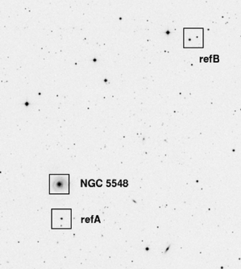
Figure 1: Digitized Sky Survey (DSS) $R$-band image of the photometric field for NGC 5548. The squares represent three $1^{\prime}.5\times 1^{\prime}.5$ fields of MIP camera. The left star (B1) in the ref B field is used for the $BVK$ images, and the right star (B2) for the $H$ image.

Digitized Sky Survey (DSS) images for four target fields are shown in Figures 1 to 4. The FWHMs of the PSF during the observations were typically $1^{\prime\prime}.0-1^{\prime\prime}.5$ in the optical and $0^{\prime\prime}.8-1^{\prime\prime}.0$ in the near-infrared. One standard star was observed each night to calibrate the flux of the reference stars. Twilight flat was obtained each evening for the $U$-band images, and dome flat for other bands was obtained at dawn after the observation. Our monitoring observations were performed with the highly automated observing system we developed (Kobayashi et al. 2003).

2.2 Reduction and Photometry

The images were reduced using IRAF. We followed the standard procedures for image reduction, with small corrections for the non-linear response of the detectors. For the infrared image reduction, a sky image assembled from dithered images pointed at the reference stars was subtracted prior to flat-fielding. Then, flat-field corrections were applied using dome flats for the optical images and illumination-corrected dome flats for the near-infrared images. Twilight flats were used for the $U$-band images.

The nuclear fluxes of the galaxies were measured relative to the reference stars, and then the fluxes of these stars were calibrated. Aperture photometry within $\phi=8^{\prime\prime}.3$ with the sky reference of $\phi=11^{\prime\prime}.1-13^{\prime\prime}.9$ ring was applied to all images, then the fluxes of the nuclei and the reference stars were compared. We adopted a large aperture rather than that generally used for a PSF-like object because the variation of the PSF during the observation increases the scatter of the flux, which often dominates the uncertainties in the aperture photometry applied for the nucleus on the extended source of the host galaxy.

For each object and band, we used two comparison methods of relative photometry considering their conditions. In one method, the average fluxes of the nuclei and the reference stars over all dithering sets were calculated before they were compared. In the other method, the fluxes of the nuclei and the reference stars were compared for each dithering set before the relative fluxes were assembled. The latter method can cancel relatively slow changes in transparency of the atmosphere during the observation, but has a statistical disadvantage because the number of the position is only six or less. We chose it mainly for the optical bands and chose the former mainly for the near-infrared bands. Rapid fluctuation of the flux between the dithering positions in the same night was attributed to thin cloud, and such observations were omitted from the light curve data.

The uncertainty in the measurements is determined as the rms variations, divided by square root of the number of frames in the first method or the number of positions in the second method, about these averages in the relative photometry. The errors for each night were usually better than $\sigma=$ 0.01 mag. The flux ratios of two reference stars $f({\rm A})/f({\rm B})$ in various bands were monitored to confirm that they were not variable.

The fluxes of the reference stars were calibrated with respect to photometric standard stars taken from Landolt (1992) and Hunt et al. (1998). The magnitudes of the reference stars were determined using fixed airmass coefficients for many data sets for which the nucleus and the standard stars were observed in the same night. The airmass coefficients were stable on clear nights, and we adopted pre-measured values of 0.212 ($B$), 0.116 ($V$), 0.016 ($J$), and 0.011 ($H$) for unit airmass. We adopted the fitted value for each calibration, ranging from 0.04 to 0.08 for the $K$ band. The calibration errors were less than 0.01 mag in most bands. The coordinates and magnitudes of the reference stars in the optical and near-infrared bands are shown in Tables 2 and 3, respectively. The aperture magnitude of the nucleus was determined each night, relative to those of the reference stars obtained each night. Small corrections for the color term in the optical filters were also applied.

The fluxes in the aperture are significantly contaminated by starlight of the host galaxy. The offset galaxy fluxes for the target AGNs were estimated as follows: The surface profile of the galaxy was fitted using GALFIT (Peng et al. 2002) where the images of the reference stars in the same night were used as the PSF. This profile was subtracted from the observed image, and the flux of the residual PSF-like image was measured. Then, the offset galaxy flux in the aperture was determined as the difference between the total flux in the aperture and the flux of the residual PSF-like image. The offset galaxy flux estimated from the data of best PSF was subtracted from the observed light curve.

In the case of NGC 7469, which has a ring-shaped star-forming region with a radius of about $1^{\prime\prime}.3$ around the nucleus, the flux of the PSF-like image was estimated without obtaining the galaxy profile with GALFIT. Instead, we estimated the nuclear flux by substracting the central PSF image from the observed image and regarding the residual at the center as the galaxy offset. A lower nuclear flux was then obtained from a larger offset by equating such residual with the brightness at the radius of the star-forming ring, while a larger nuclear flux from a lower offset by equating such residual with the brightness at the radius outside which the galaxy profile dominates over the profile of star-forming ring.

The offset galaxy fluxes thus estimated in the $\phi=8^{\prime\prime}.3$ are given in Table 4. Their uncertainty estimated from the scatter over different nights or the residual flux at the origin of the flux to flux diagram is $10-30$ %, sometimes giving a significant error in the nuclear flux which may result in false variations of the nuclear color. Note that the galaxy subtraction provides an offset flux only and does not affect the cross-correlation analysis in §4.

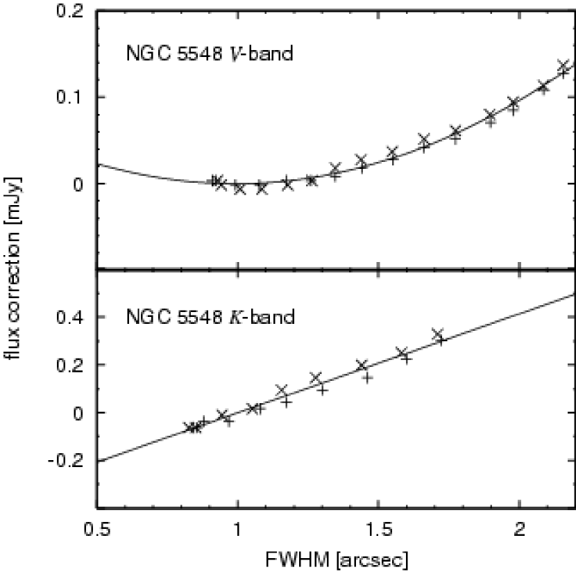
Figure 5: Correction of nuclear flux for the seeing effect, scaled to be zero at ${\rm FWHM}=1^{\prime\prime}$, for some example cases of NGC 5548. Seeing-dependence of nuclear flux is simulated by convolving the image of good seeing conditions with the FWHM chosen. Different symbols show the simulated results for different epochs. Thick lines are the fitting curves.

The host galaxy flux in the aperture depends on the seeing FWHM. This effect makes a systematic change in the measured nuclear flux up to 0.03 mag depending on the central profile of the host galaxy, and causes false fluctuations in the light curve. In order to estimate a relation between the seeing FWHM and the corresponding nuclear flux, the images in the best seeing condition were convolved with several FWHM values, as shown in Figure 5. Thus, the nuclear flux measured each night was corrected using the fitting formulae:

$$\Delta F=a({\rm FWHM}-1)+b({\rm FWHM}-1)^{2}\;\;[{\rm mJy}],$$ (1)

where $a$ and $b$ are the constants and their values for each nucleus and band are given in Table 5. However, such correction was not attempted in the cases of $BJH$ for NGC 4051 and $BVJHK$ for NGC 3227, because the photometric errors of each night were found to dominate over the seeing effect.

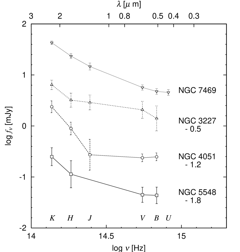
Figure 6: Optical to near-infrared spectral energy distributions (SEDs) for the target nuclei, where the host galaxy contribution has been subtracted. The fluxes shown are averaged over all observing nights. The error bars include the rms flux variations and subtraction errors. The number below each object name is the offset value to log$f_{\nu}$.

Figure 6 shows the spectral energy distribution (SED) observed in the optical ($UBV$) and near-infrared ($JHK$) for each nucleus. The fluxes are those averaged over the nights when the SEDs were observed. The error bars include their rms variations and the uncertainties in the offset subtraction. We see that the SED is steep in the near-infrared ($JHK$) while it is flat in the optical ($UBV$) except for NGC 3227. This is consistent with a view that the hot dust emission dominates towards longer wavelengths in the near-infrared, while the flat power-law spectra from nuclei of Seyfert galaxies dominates in the UV and optical. However, NGC 3227 shows a steep SED in the optical which is different from the other nuclei. This may originate from offset errors in the $V$ band (see §3.2), rather than originating from the central engine .

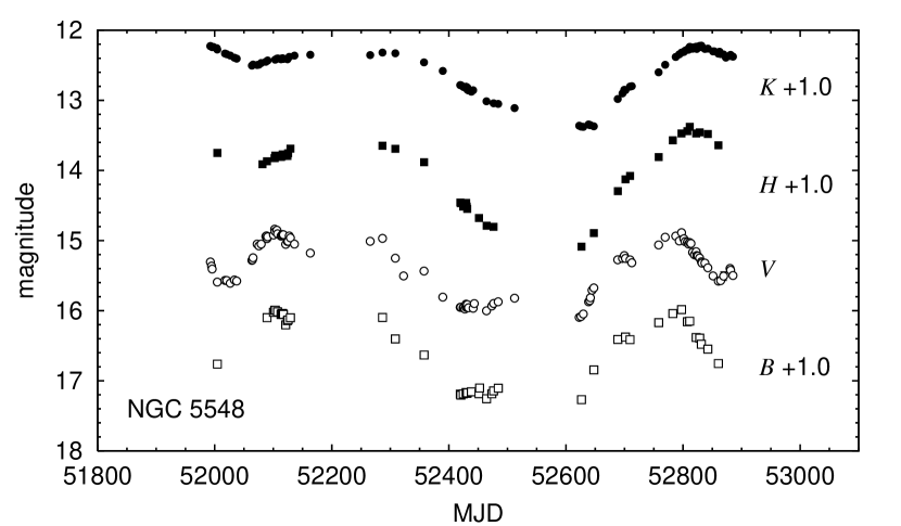
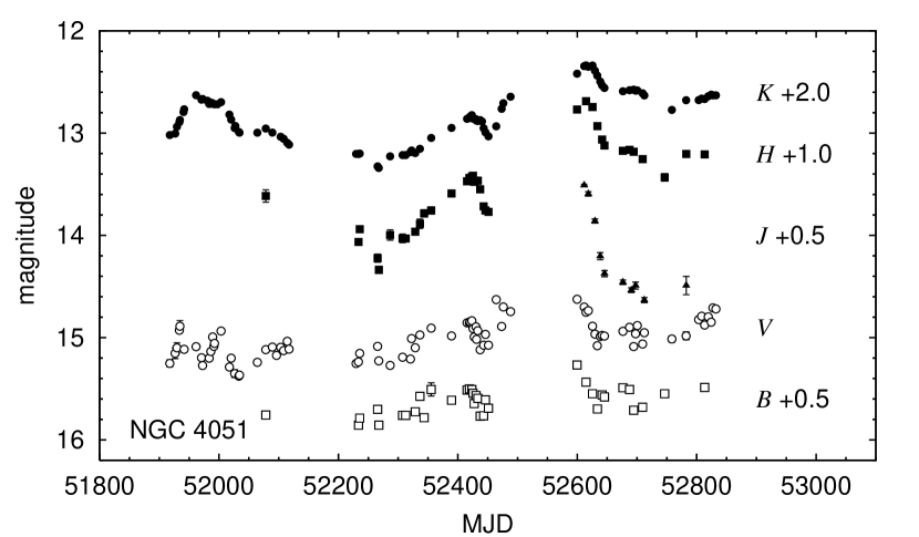
Figure 7: Observed $BVHK$ light curves of NGC 5548 nucleus for the period from March 2001 to September 2003.

Figure 8: Observed $BVJHK$ light curves of NGC 4051 nucleus for the period from January 2001 to July 2003.

The light curves based on aperture fluxes of four target AGNs are shown in Figures 8 to 10. The correction for the seeing effect has been applied and the offset flux of the host galaxy has been subtracted here.

3 Features of Optical and Near-infrared Variations

3.1 Data

The sampling characteristics of the $V$ and $K$ light-curve data are given in Table 6. The whole monitoring period for each galaxy and the maximum intervals between adjacent sampling epochs are given in columns 2 and 3, respectively. The number of data points, the average and median intervals for the $V$ band are given in columns 4, 5 and 6, respectively, and those for the $K$ band are in columns 7, 8 and 9. The maximum interval corresponds to the sampling gap due to solar conjunction. The average interval is longer than the median, because of sampling gaps of three months due to solar conjunction and occasional blanks of several weeks caused by bad weather or facility maintenance. The median interval of $3-5$ days over $2-3$ years is much shorter than any other monitoring observations in the near-infrared. Because of changing weather conditions and/or sudden problems with instruments, there are cases where the observations in the $V$ band were successful while not in the $K$ band, and vice versa. Therefore, the number of $V$-band data points does not necessarily coincide with that for the $K$ band.

The statistics that characterize the observed variability in the $V$ and $K$ bands are given in Table 7. The values in this table were calculated after the offset flux of the host galaxy in the aperture was subtracted. For each target AGN, the average flux $\left<f\right>$, the maximum to minimum flux ratio $R_{\rm max}$, and the normalized variability amplitude $F_{\rm var}$ are given. Here, we define $F_{\rm var}$ as the variance of the flux $\sigma$, corrected for the measurement uncertainty $\delta$, divided by the average flux:

$$F_{\rm var}=\frac{\sqrt{\sigma^{2}-\delta^{2}}}{\left<f\right>}\;\;\;,$$ (2)

where

$$\sigma^{2}=\frac{1}{N}\sum_{i=1}^{N}(f_{i}-\left<f\right>)^{2}\;\;\;,$$ (3)

and

$$\delta^{2}=\frac{1}{N}\sum_{i=1}^{N}\delta_{i}^{2}\;\;\;.$$ (4)

It is evident from the values of $F_{\rm var}$ in this table that the four AGNs underwent significant $V$ and $K$ variations during our monitoring observations.

3.2 Optical Variation

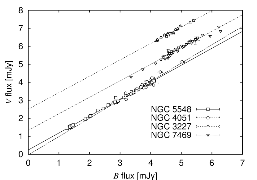
Figure 11: The flux-to-flux diagram where the $V$ flux is plotted against the $B$ flux for the target AGNs. The host galaxy flux, given in Table 4, has been subtracted from the nuclear flux. The error bars correspond to the errors of differential photometry in deriving the light curves. Lines represent linear regressions.

Comparison of flux variations between the $B$ and $V$ bands for each AGN indicates that their long timescale variations as well as small, short timescale fluctuations are almost synchronized (Figures 8 to 10). This tendency is also true of the $U$-band variations for NGC 7469. Figure 11 shows the $V$ flux plotted against the $B$ flux for each AGN. Each point represents a pair of nuclear fluxes in a certain night from which the flux of the host galaxy has been subtracted, and the error bars represent the photometric errors. There is a tight linear relation between the flux variations in the $B$ and $V$ bands.

Winkler et al. (1992) and Winkler (1997) reported this linear relation between the optical flux variations for many Seyfert galaxies in the southern hemisphere. They considered that the slope of the linear relation in the flux-to-flux diagram, called a flux variation gradient (FVG), would represent the actual color of the variable component, which appears to be constant for individual AGNs. If this is the case, the offset of the linear regression line from the origin is due to non-variable components, such as errors in subtracting the galaxy flux, unresolved narrow-line fluxes, etc.

A tight linear relation and no sign of significant non-linearity in Figure 11 support the above view, and the color of the central engine derived from the FVG, which is unaffected by non-variable components, would be more reliable than those inferred from the SED in Figure 6. Our estimate of nuclear $B-V$ color from the FVG, after being corrected for Galactic extinction, gives $(B-V)_{\rm FVG}=0.04\pm 0.01$ (NGC 5548), $0.13\pm 0.05$ (NGC 4051), $0.00\pm 0.04$ (NGC 3227), and $-0.04\pm 0.03$ (NGC 7469). These values are similar to a typical value for Seyfert 1 galaxies reported by Winkler et al. (1992), and correspond to the power-law nuclear flux $f_{\nu}\propto\nu^{\alpha}$ with $\alpha=+0.36\pm 0.03$ (NGC 5548), $-0.04\pm 0.22$ (NGC 4051), $+0.53\pm 0.17$ (NGC 3227), and $+0.70\pm 0.11$ (NGC 7469), provided the effects of emission-line fluxes such as H$\beta$ are not taken into account.

3.3 Near-infrared Variation

In contrast with the optical light curves showing the short-term fluctuations, the near-infrared light curves in the $JHK$ bands are smooth (Figures 8 to 10). This is consistent with a view that the bulk of near-infrared emission comes from the thermal reprocessing region whose size exceeds the distance over which light travels in the timescale of short-term fluctuations in the optical.

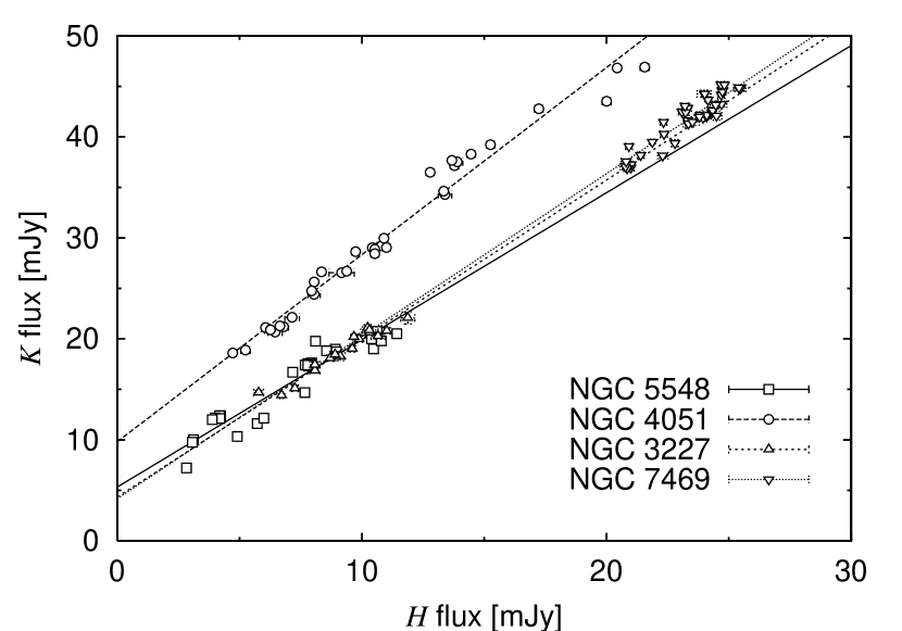
Figure 12: The flux-to-flux diagram. The same as Figure 11, except that the $K$ flux is plotted against the $H$ flux for the target AGNs.

Figure 12 shows the $K$ flux plotted against the $H$ flux for each AGN. There is a linear relation between the flux variations in the $K$ and $H$ bands. Our estimate of nuclear $H-K$ color from the FVG gives $(H-K)_{\rm FVG}=0.92\pm 0.07$ (NGC 5548), $1.17\pm 0.04$ (NGC 4051), $1.00\pm 0.06$ (NGC 3227), and $1.02\pm 0.07$ (NGC 7469), which is consistent with the FVG colors for dozens of Seyfert galaxies measured by Glass (2004). These colors correspond to the black-body temperature of $1500-1800$ K which agrees with the sublimation temperature of graphite grains, and support the thermal origin of near-infrared emission, especially in the $K$ band.

There is a scatter in the FVG in Figure 12, and the relation between the $H$ and $K$ flux variations is not as tight as that for the $B$ and $V$ fluxes. This implies that the thermal reprocessing region that emits the $H$ flux may not completely coincide with that for the $K$ flux, and/or the central source could contaminate differently in the $H$ and $K$ fluxes.

3.4 Correlation and Lag time between Optical and Near-infrared Variations

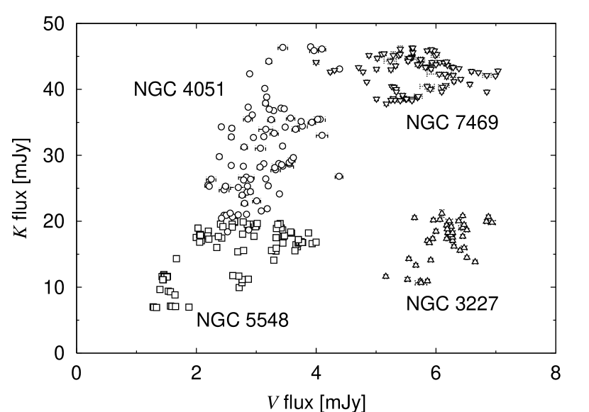
Figure 13: The flux-to-flux diagram. The same as Figure 11, except that the $K$ flux is plotted against the $V$ flux for the target AGNs.

The most important feature of the near-infrared variation, besides its smoothness, is its lag time behind the optical variation. Figures 8 to 10 show that the near-infrared light curve resembles the optical light curve, if shifted backwards by about ten days (NGC 4051 and NGC 3227) or several tens of days (NGC 5548 and NGC 7469). Figure 13 shows the $K$ flux plotted against the $V$ flux for each AGN. Because of the short-term fluctuations present only in the $V$ band, and because of the delay between the $V$ and $K$ variations, there is a significant scatter in Figure 13.

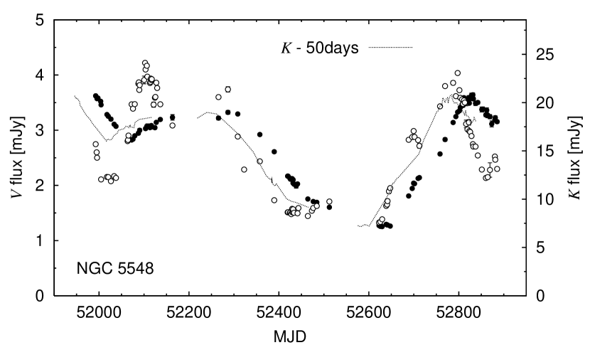
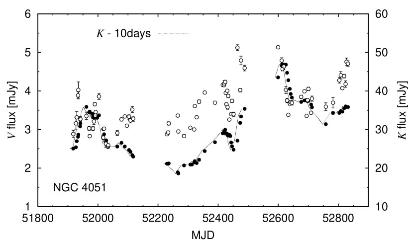
Figure 14: Observed $V$ and $K$ light curves of NGC 5548 nucleus. Open and filled circles correspond to $V$ and $K$, respectively. The dotted line is the $K$ light curve shifted backwards by 50 days.

Figure 15: Observed $V$ and $K$ light curves for NGC 4051 nucleus. Others are the same as Figure 15, but for the shift by 10 days.

The lag time is approximately estimated by shifting either one of the $V$ or $K$ light curves horizontally. Figures 15 to 17 show the observed $V$ and $K$ light curves for each AGN. The dotted curve in each figure is the $K$ light curve shifted backwards by the lag time determined approximately by sight. A more reliable estimate of lag time will be given in the next section.

4 CROSS-CORRELATION ANALYSIS

Quantitative estimates of lag time between the optical and near-infrared light curves are possible based on the cross-correlation analysis commonly used in studies of multiple time series. For example, the application of this type of analysis to spectroscopic monitoring observations of broad emission lines dates back more than a decade (for a review, see Peterson 2001).

Let $C(t)$ and $I(t)$ be the irradiating ($V$ band) and responding ($K$ band) light curves at time $t$, respectively. Then they are related to each other via

$$I(t)=\int\Psi(\tau)\;C(t-\tau)d\tau\;\;,$$ (5)

where $\Psi(\tau)$ is the transfer function with respect to the lag time $\tau$. This equation indicates that the transfer function represents the time-smeared response to a $\delta$-function outburst of incident radiation.

As a function of lag time $\tau$, the cross-correlation function (CCF) and the auto-correlation function (ACF) are defined, respectively, as

$${\rm CCF}(\tau)=\int I(t)C(t-\tau)dt\;\;,$$ (6)

and

$${\rm ACF}(\tau)=\int C(t)C(t-\tau)dt\;\;\;.$$ (7)

The ACF is therefore the cross-correlation of the incident light curve with itself. Use of equation 5 to replace $I(t)$ in equation 6 gives

$${\rm CCF}(\tau)=\int\Psi(\tau^{\prime}){\rm ACF}(\tau-\tau^{\prime})d\tau^{\prime}\;\;\;.$$ (8)

The CCF is therefore the convolution of the transfer function with the ACF.

The cross-correlation does not necessarily give an unambiguous measure of $\Psi(\tau)$, but simply quantifies the time delay $\tau$ between the two light curves, which approximately represents the location of the peak or the centroid of $\Psi(\tau)$. For intuitive interpretation of the CCF, we rewrite equation 6 as follows:

$${\rm CCF}(\tau) = \frac{1}{2}\int I(t)^{2}dt\;+\;\frac{1}{2}\int C(t-\tau)^{2}dt$$ (9)

$$- \;\frac{1}{2}\int\left[I(t)-C(t-\tau)\right]^{2}dt\;\;\;.$$

The first and second terms are nearly constant, if the interval of time integration is much larger than $\tau$. Therefore, the third term, which is an integration of square difference between $I(t)$ and $C(t-\tau)$, determines the shape of CCF($\tau$). We see that the CCF becomes maximum when the third term becomes minimum. Equation 9 supports our sight estimation of lag time by shifting either one of the irradiating and responding light curves with respect to time (Figures 15 to 17), if two light curves are linearly related to each other.

The CCF is equivalent to the correlation coefficient for the pairs of time series $(C(t-\tau),I(t))$. Thereby, practical calculation is given by

$${\rm CCF}(\tau)=\frac{1}{N}\sum_{i=1}^{N}\frac{[\,C(t_{i}-\tau)-\left<C\right>\,][\,I(t_{i})-\left<I\right>\,]}{\sigma_{C}\,\sigma_{I}}\;\;,$$ (10)

where $N$ is the number of pairs, and $\left<C\right>$ and $\left<I\right>$ are the averages of $C(t-\tau)$ and $I(t)$, respectively, and $\sigma_{C}$ and $\sigma_{I}$ are their standard deviations. Note that this equation is valid only for the period during which $C(t-\tau)$ and $I(t)$ overlap in time.

4.1 Interpolation Scheme

The data points in equation 10 should be regularly spaced in time, because each point in one light curve must be paired with a corresponding point in the other. For generating the pairs $(C(t-\tau),I(t))$, or equivalently $(V(t-\tau),K(t))$ in our case, linear interpolation of either one of the $V$ or $K$ light curves has generally been used with small modifications if necessary (e.g., Gaskell & Peterson 1987; White & Peterson 1994).

This interpolation method, however, sometimes does not provide a sufficient number of pairs for calculation, so that the shape of CCF is noisy and its peak difficult to detect. Furthermore, this method does not guarantee a symmetrical ACF with respect to a lag time of zero, when the sampling of the data has a highly unbalanced weight for time.

Here, we calculate CCFs based on different methods of interpolation, “bidirectionally interpolated” (BI) CCFs and “equally sampled” (ES) CCFs. Let $\{V_{1},V_{2},...,V_{N}\}$ and $\{K_{1},K_{2},...,K_{M}\}$ be the fluxes of two observed light curves irregularly sampled at times $\{t_{1},t_{2},...,t_{N}\}$ and $\{t^{\prime}_{1},t^{\prime}_{2},...,t^{\prime}_{M}\}$, respectively. Then, for the data pairs for which we calculate the standard linear correlation coefficient for lag time $\tau$, BI-CCFs combine two types of pairs, ($V_{i},K_{\rm{int}}(t_{i}+\tau)$) and ($V_{\rm{int}}(t^{\prime}_{j}-\tau),K_{j}$), where $V_{\rm{int}}$ and $K_{\rm{int}}$ are linearly interpolated fluxes from $\{V_{1},V_{2},...,V_{N}\}$ and $\{K_{1},K_{2},...,K_{M}\}$, respectively. ES-CCFs collect the pairs of ($V_{\rm{int}}(t),K_{\rm{int}}(t+\tau)$), where $t$ is sampled by equal interval $\Delta t$ independent of $\{t_{1},t_{2},...,t_{N}\}$ and $\{t^{\prime}_{1},t^{\prime}_{2},...,t^{\prime}_{M}\}$.

These two methods provide symmetrical ACFs with respect to a lag time of zero. The BI-CCFs put weight on the observed data, yet are affected by the unbalanced sampling of observations concurrently. The ES-CCFs have contrary characteristics. The problem in the interpolation, which occurs inevitably in both BI and ES methods, can be overcome by simulation of flux variations, as described below.

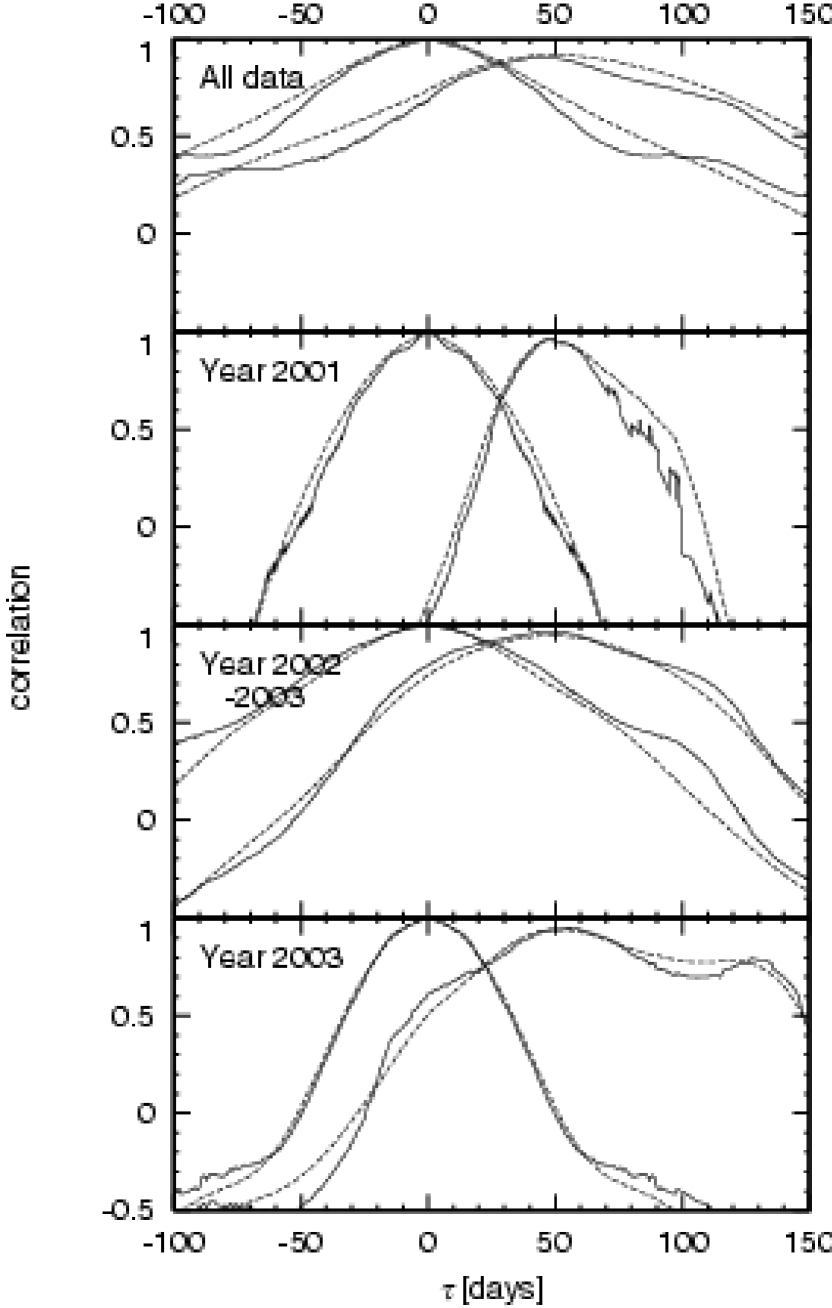
Figure 18: CCFs and ACFs for various monitoring periods of NGC 5548. The $V$ and $K$ light curves are used to calculate the CCFs. The $V$ light curve is used to calculate the ACFs that are symmetrical on either side of $\tau=0$. The solid and dashed lines are the results based on the BI and ES methods, respectively.

Figures 18 to 21 show the CCFs and ACFs for four target AGNs calculated by the two methods of BI and ES. Table 8 shows the cross-correlation results for several subsets of the observed light curve data used in the calculation. The monitoring period for each subset, expressed in the modified Julian date (MJD), is given in column 3. The CCF peak position $\tau_{\rm peak}$ and the CCF peak value $r_{\rm max}$ for the BI method are in columns 5 and 6, respectively, and those for the ES method are in columns 7 and 8.

4.2 Uncertainty of Lag time

Monte Carlo simulations are reliable for quantitative estimates of lag time. Maoz & Netzer (1989) introduced the basic scheme for this type of simulation. A large number of artificial light curves are created for both irradiating and reprocessing sources, and their CCFs are calculated to determine the peak position $\tau_{\rm{peak}}$ for each pair of light curves. The empirical distribution of $\tau_{\rm{peak}}$ is called ‘cross-correlation-peak-distribution (CCPD)’. The uncertainty of lag time is determined from the CCPD.

In this technique, it is important to simulate the light curve such that the causes of the uncertainty should be adequately reflected in the uncertainty of lag time. There are two major sources of uncertainty in lag time measurements. One is flux errors in individual data points, and the other is the sampling gaps that often significantly underestimate the real variations. In our photometric monitoring data, the former is not effective, because the photometric data have been obtained from homogeneous observation with very high S/N ratios, especially for nearby Seyfert galaxies. On the other hand, the latter seriously affects the analysis, because there are inevitable gaps of three months due to solar conjunction and blanks of a few weeks due to bad weather conditions or facility maintenance.

Artificial light curves should be simulated in a less model-dependent way, based on the observed light curves, because we have a limited knowledge of the variability mechanism in the $V$ band and the transfer function from the $V$-band variations to the $K$-band variations. Peterson et al. (1998) introduced a model-independent Monte Carlo method, called “flux randomization/random subset selection (FR/RSS)”, where the simulated light curve is based on the observed one.

The FR method modifies the observed fluxes in each simulation by random Gaussian deviations based on the quoted error of each observed point, and accounts for the effects of flux-measurement uncertainties. The RSS method randomly extracts the same number of data points from the observed light curve, allowing for multiple extraction, to construct an artificial light curve. This method is then able to estimate the uncertainty due to the different time sampling of the data points. However, multiple extraction results in the removal of the observed data points at certain times in each simulation, which underestimates the real variation of the light curve.

Here we introduce a new technique of realizing the light curves, which simulate the flux variations between the observed data points using stochastic processes characterized by the structure function (SF) from the observed light curves. The SF is often used for the analysis of single time series (Simonetti et al. 1985). It measures the distribution of power over timescales for which the variations are correlated. A first-order structure function, for a series of flux measurements $f(t_{i})$, $i=1,2,3,....$ is defined as

$$S(\tau)=\frac{1}{N(\tau)}\sum_{i<j}\left[f(t_{i})-f(t_{j})\right]^{2}\;\;,$$ (11)

where the sum is over all pairs for which $t_{j}-t_{i}=\tau$, and $N(\tau)$ is the number of pairs. The SF of most AGNs is given by

$$S(\tau)=S_{0}\;\tau^{\beta}\;\;,$$ (12)

which increases up to some characteristic lag time of months or years.

At first, the mean square variation $\sigma^{2}(dt)$ in regard to interval $dt$ is determined based on the SF of the observed light curve. In simulation of each light curve, an epoch during a sampling gap is randomly determined, and the flux is generated by random Gaussian deviations, which is equivalent to the FR method except for using the variability parameter $\sigma^{2}(dt)$ from the linearly interpolated flux from the observed data points. Once the point is achieved, it is regarded as an observed data point in the light curve, so that the realized data should have self-correlation seen in the observed light curves. Similar efforts are repeated until the mean sampling interval of the updated light curve decreases to one day. The light curve, generated this way, is used in each CCF method, instead of using the interpolated fluxes in either of $V_{\rm{int}}$ or $K_{\rm{int}}$.

4.3 Calculation and Simulation

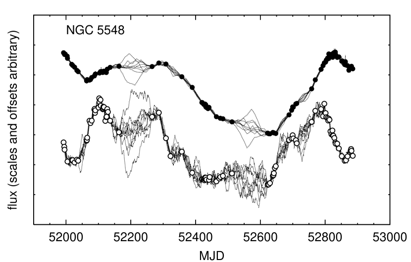
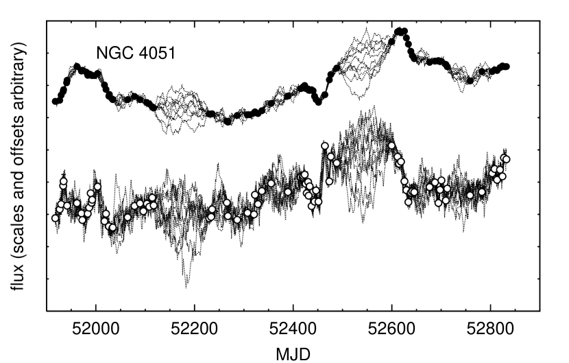
Figure 22: Simulated $V$ and $K$ light curves of NGC 5548. Lower and upper dotted lines correspond to $V$ and $K$, respectively. Open and filled circles represent the observed $V$ and $K$ data points, respectively.

Figure 23: Simulated $V$ and $K$ light curves of NGC 4051. Others are the same as Figure 23.

Table 9 shows the SFs fitted by equation 12 using all the observed data in the $V$ and $K$ bands for each target AGN. The mean square variation $\sigma^{2}(dt)$ is determined directly from the observed SF. However, in a particular case of the $K$ band for NGC 5548, it was determined as $\sigma^{2}(dt)=10\times(dt/60{\rm days})^{3}$ $({\rm mJy})^{2}$, by iteration until the simulated SF agrees with the observed SF. In this way we generated 1000 pairs of artificial $V$ and $K$ light curves, some of which are shown in Figures 23 to 25, together with the observed data.

The lag time was calculated for each subset of the monitoring period, because we are interested in whether phase-to-phase changes in lag time exist, and also because we know that the variation in the $K$ band does not always respond linearly to that in the $V$ band. The lag time for the entire monitoring period was also calculated, but this is only for reference.

In principle, the lag time was calculated from the data taken over a period between two adjacent solar conjunctions. Only for NGC 5548, we combined the second season of Year 2002 and a part of the third season of Year 2003, so that the lag time was calculated over a full period including the minimum luminosity state.

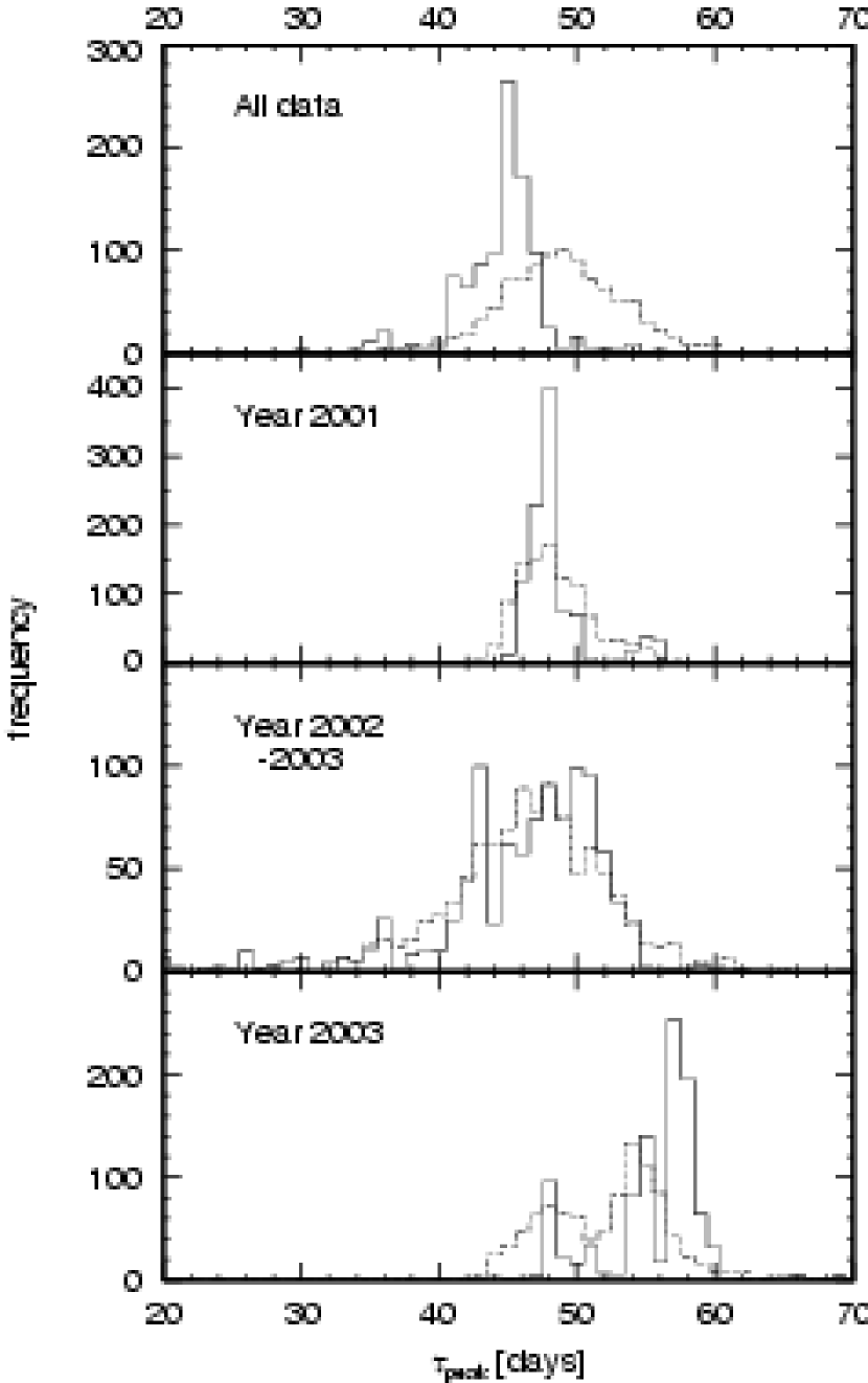
Figure 26: CCPDs for various monitoring periods of NGC 5548. The histogram shows the number of our simulation runs in each bin of $\Delta\tau_{\rm peak}=2$ days. The solid and dotted lines are the results based on the BI and ES methods, respectively.

The CCPDs from Monte Carlo simulations are shown in Figures 26 to 29, where the frequency distribution of $\tau_{\rm{peak}}$ over simulation runs is plotted as a histogram. Here, such runs of low CCF peaks with confidence levels of less than 95 % are excluded, where the confidence level is derived from the peak value of CCF and the number of observed data points in the overlapping period of the two time series shifted after by $\tau$.

Table 10 shows the cross-correlation results from the simulated light curves. The lag time was determined as a median of $\tau_{\rm{peak}}$, or 50 % fraction of the cumulative CCPD. The uncertainty is measured by $\pm$34.1 % fraction from the median, thus corresponding to 1$\sigma$ error for a normal statistical distribution.

The lag time for NGC 4051 needs careful interpretation. There are two comparable peaks in the CCF, located at $\tau_{\rm peak}=10-20$ days and $50-100$ days. For the latter case, however, the major ascending and descending parts of the $K$ light curve are shifted into the blank periods of the $V$ light curve, so that the high correlation may not be real. The rapid $V$-band variations on short timescales of up to a month are not at all correlated with the $K$-band light curve if shifted backwards by $50-100$ days. According to equation 9, the $V$ and $K$ variations of larger amplitude and longer timescale in the overlapping period tend to maximize the CCFs more effectively by chance, even if those of shorter timescale are in fact highly correlated. It is very likely that the global flux variation for NGC 4051 contains information on some other effect of time shift in addition to the light-travel effect. Considering the above, the lag time shown in the table is calculated from the histogram below the dip at $\tau_{\rm peak}\approx 42$ days.

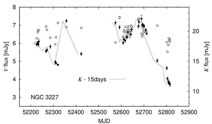
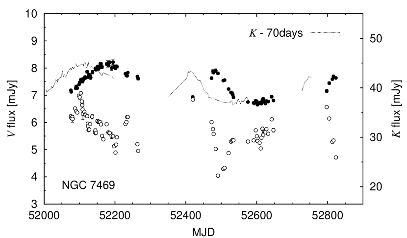
Figure 16: Observed $V$ and $K$ light curves for NGC 3227 nucleus. Others are the same as Figure 15, but for the shift by 15 days.

Figure 17: Observed $V$ and $K$ light curves for NGC 7469 nucleus. Others are the same as Figure 15, but for the shift by 70 days.

We detected the lag time for NGC 3227 for the first time, though the uncertainty is not very small. As seen from Figure 17, the optical variation of NGC 3227 is very rapid like that of NGC 4051. The light curve data are undersampled because of some unfortunate gaps, especially in 2003. More observations are needed to accurately measure the lag time for such an AGN with low-luminosity and rapid optical variation.

There is a possibility that the lag time may be underestimated, not representing the light-travel time from the central engine to the hot dust region. The contribution of the $K$-band flux from the central engine, if any, would make the phase of near-infrared variations closer to the corresponding phase in the optical. In this case, the lag time should be systematically smaller than the light-travel time from the central engine to the hot dust region. If the power-law optical component from the central engine is extended to the near-infrared wavelength region, its maximum contribution in the $K$-band flux is about 10 %. Subtraction of this component from the $K$-band flux observed on the same night would increase the lag time by $10-20$ %.

5 DISCUSSION

In most cases, the CCPDs are smooth and have clear peaks, and a lag between the $V$ and $K$ variations is detected (Figures 26 to 29). Generally, BI-CCFs tend to have a sharp jump, in contrast to ES-CCFs for which the pairs are sampled densely and constantly. Such a jump appears close to the peak and affects the values of $\tau_{\rm peak}$. We therefore use the ES-CCF result in Table 10 as representing the lag time in following discussions. Note that the lag time for all data is only for reference and is not shown in the plots.

5.1 Relation between Infrared Lag and Central Luminosity

The dust reverberation models, applied to previous observations of AGNs, have estimated an equilibrium temperature at the inner radius of the dust torus (Clavel, Wamsteker & Glass 1989; Nelson 1996), which is consistent with the thermal emission in the near-infrared originating from the hot dust heated at its sublimation temperature in the range of $1300-2000$ K (Barvainis 1992). As a result, there would be an inner hole of hot dust torus whose radius is proportional to a square root of central luminosity. The lag time between UV/optical continuum variations and near-infrared ($\sim$2 $\mu$m) continuum variations should be the light-travel time from the center to the dust region.

Our lag measurements of the four AGNs (NGC 5548, NGC 4051, NGC 3227, NGC 7469) are given in Table 10, and are plotted against the absolute $V$ magnitude in Figure 30, together with previous measurements. The filled symbols are our results, including our early result for NGC 4151 (Minezaki et al. 2004). The others are taken from the literature (see Minezaki et al. 2004 and references therein). It is evident from this figure that a good correlation of $\Delta t\propto L^{0.5}$, indicated earlier from $M_{V}=-23$ to $-18$ by Minezaki et al. (2004), now extends down to $M_{V}=-15$, spanning a range of 1000 times in luminosity.

In particular, we have expanded the range of $M_{V}$ faintwards by about three magnitudes by measuring, for the first time, the lag time of NGC 4051 which sits in the faint end of “classical” Seyfert nuclei. This indicates that AGNs of low luminosity might also have the dust torus expected from the dust reverberation models.

The good correlation between lag time and absolute $V$ magnitude strongly supports our idea of using $\Delta t\propto L^{0.5}$ as a distance indicator for AGNs (Kobayashi et al. 1998b; Yoshii 2002).

Given a narrow range of flux variations throughout our monitoring period, we could not find clear differences among successive lag measurements for individual AGNs. Observations covering larger flux variations are desirable for investigating how the hot dust would be redistributed against changes in the power of the central engine.

5.2 Relation between Infrared Lag and Central Mass

One of other fundamental quantities that characterize AGNs is the central mass, which could be regarded as the mass of a super-massive black hole. For the high-energy region, comparison of the characteristic frequency of X-ray variability power spectra of AGNs with that of black hole X-ray binaries has led to an interpretation that the size of the X-ray-emitting region would linearly scale with gravitational radius or gravitational mass, so that the X-ray variability has been proposed as a method of measuring the mass of AGNs (Hayashida et al. 1998; Uttley et al. 2002). For the UV or optical region, the optically thick and geometrically thin accretion disk is generally believed to be a source of UV and optical continuum from AGNs, and the standard model expects a radial temperature distribution in the disk that depends on both accretion rate and central mass (Frank, King, & Raine 1992). Therefore, it is worthwhile to examine how the inner radius of the dust torus scales with central mass.

Recent measurements of lag time and velocity dispersion for several broad emission lines in NGC 5548 have given evidence for Kepler motion of the BLR gas (Peterson & Wandel 1999). Assuming that the virial theorem applies similarly to about three dozen Seyfert nuclei and quasars that have been targets of reverberation mapping observations for the BLR (e.g., Wandel, Peterson & Malkan 1999; Kaspi et al. 2000; Peterson et al. 2004), their central masses have been estimated with a typical uncertainty of a factor of 2 or 3 over a range of $10^{6}-10^{8}M_{\odot}$.

Figure 31 shows the infrared lag measurements plotted against the central masses that have been measured from reverberation radii and widths of broad emission lines in individual AGNs. The meanings of filled and open symbols are the same as in Figure 30 for infrared lag measurements. The central masses are taken from Peterson et al. (2004). The inclined lines correspond to $c\Delta t/R_{g}=10^{3}$, $10^{4}$, $10^{5}$, and $10^{6}$, where $c\Delta t$ is the light-travel distance or inner radius of the dust torus, and $R_{g}=GM_{c}/c^{2}$ is the gravitational radius which scales linearly with central mass $M_{c}$.

Correlation between the central mass and the lag time (Figure 31) is weaker than between the central optical luminosity and the lag time (Figure 30). Furthermore, the inner radius of dust torus $c\Delta t$ does not scale with gravitational radius $R_{g}$ that encloses the central mass. It is therefore evident that the inner radius of dust torus is not determined by the dynamics under the influence of a supermassive black hole at the center, but rather by the strength of UV/optical radiation from the central engine. As a consequence, the scatter in Figure 31 might be interpreted as the difference in mass-to-luminosity ratio that should be determined by the accretion rate and the radiative efficiency in accretion flow in individual AGNs.

5.3 Relation of Dust Torus with Broad Line Region

Confirmation of a dust torus outside the BLR not only verifies the unification scheme of AGNs, but also yields knowledge of physical conditions in the central regions of AGNs for which we cannot yet obtain spatially resolved images. Previously, Clavel, Wamsteker & Glass (1989) measured both BLR and dust reverberation radii during the same monitoring campaign for a bright Seyfert 1 galaxy of Fairall 9, and concluded that the hot dust is outside the BLR. We now examine whether this view is supported by our measurements of infrared lags.

Figure 32 shows our measurements of infrared lags (NGC 5548, NGC 4051, NGC 3227, NGC 7469; NGC 4151, Minezaki et al. 2004), together with previous measurements of broad-line lags in the literature (Fairall 9, Clavel, Wamstekar & Glass 1989, Rodriguez-Pascual et al. 1997, Peterson et al. 2004; NGC 3783, Reichert et al. 1994; NGC 7469, Wanders et al. 1997, Kriss et al. 2000, Collier et al. 1998; NGC 5548, Krolik et al. 1991, Peterson & Wandel 1999, Dietrich et al. 1993, Korista et al. 1995; NGC 4151, Clavel et al. 1990, Maoz et al. 1991, Kaspi et al. 1996; NGC 3227, Winge et al. 1995, Onken et al. 2003; NGC 4051, Shemmer et al. 2003). The optical luminosities corresponding to the broad-line lags are averaged over the monitoring period in each item in the literature.

Each AGN has a range of lag time for the BLR depending on the broad emission line used (Korista et al. 1995; Peterson & Wandel 1999; see also Figure 32). In general, there is a tendency for broad emission lines of higher ionization to have smaller lag times, and for those of lower ionization to have larger lag times, which suggests that the BLR has a radially stratified ionization structure. Therefore, the BLR extends out to the light-travel distance corresponding to the largest lag time in each AGN. We note that a correlation of $\Delta t\propto L^{0.7}$ has been suggested for broad H$\beta$ emission lines for a wide range of central luminosity of AGNs including quasars brighter than $M_{V}\sim-23$ (Kaspi et al. 2000), although their lags for Seyfert galaxies show a fairly large scatter.

Figure 32 shows that the lag times for broad lines are located below the boundary set by the infrared $\Delta t$ versus $M_{V}$ relation. Some lags of broad emission lines are beyond the infrared lag in the same AGN. However, this occurs when such lags for the BLR were measured in a bright state, while the infrared lag for hot dust was measured in a faint state. Such lags for the BLR, after being corrected for their luminosity dependence, become smaller than the infrared lag, as actually reported for NGC 5548 (Suganuma et al. 2004).

Thus, the outer radius of BLR nearly corresponds to the inner radius of the dust torus. In other words, it is suggested that the bulk of the emitting region of high-velocity gas is restricted inside the “wall” of the dust torus which is located at a distance determined by the continuum luminosity. Netzer & Laor (1993) proposed that the dust in the narrow line-emitting gas might separate the BLR from the NLR by suppressing the emission lines in the dust region, and that this might explain the large difference in observed properties of broad and narrow emission lines, such as line width and covering factor. The result presented in Figure 32 supports their view that the BLR size is determined by the dust sublimation radius.

5.4 Optical Delay behind X-ray Variation in NGC 5548

It has been proposed that the UV/optical flux variation in AGNs originates in the thermal reprocessing of X-ray variability by the optically thick and geometrically thin accretion disk in its outer part, while the bulk of the steady component is generated by viscous processes in the accretion disk itself (e.g., Collin-Souffrin 1991). In this scheme, the variation of reprocessed component in the UV/optical flux should show a lag time of days or less behind the variation of X-rays released from the geometrically thick hot corona in the inner part of the accretion disk.

For NGC 5548, Clavel et al. (1992) reported a UV lag of $\Delta t=0\pm 6$ days behind the X-ray, by comparing the light curves in the hard X-ray ($2-10$ keV) and the UV (1350 Å). It is not easy to detect a clear correlation between X-ray and UV/optical variations on short timescales, nor the lag time between them, because generally the amplitude of UV/optical variation on a short timescale is small and difficult to observe.

From observations of optical (5100 Å) and hard X-ray ($2-10$ kev) fluxes of light curves spanning six years for NGC 5548, Uttley et al. (2003) reported a strong correlation in their long-timescale variation, while only weakly restricting $\Delta t=0\pm 15$ days. Since the amplitude of such optical variation is found to exceed that of hard X-ray, they argued that X-ray reprocessing is not a main driver of the long-timescale optical variation, at least for NGC 5548.

Thus, the problem yet to be answered is whether there is a clear correlation between X-ray and optical variations on short timescales. As shown below, because of accurate photometry and frequent sampling of the $V$-band light curve data, we detected, for the first time, the day-basis optical variation having a small amplitude and a clear lag time behind the X-ray variation, which is well within a framework of reprocessing the X-ray flux into the optical flux.

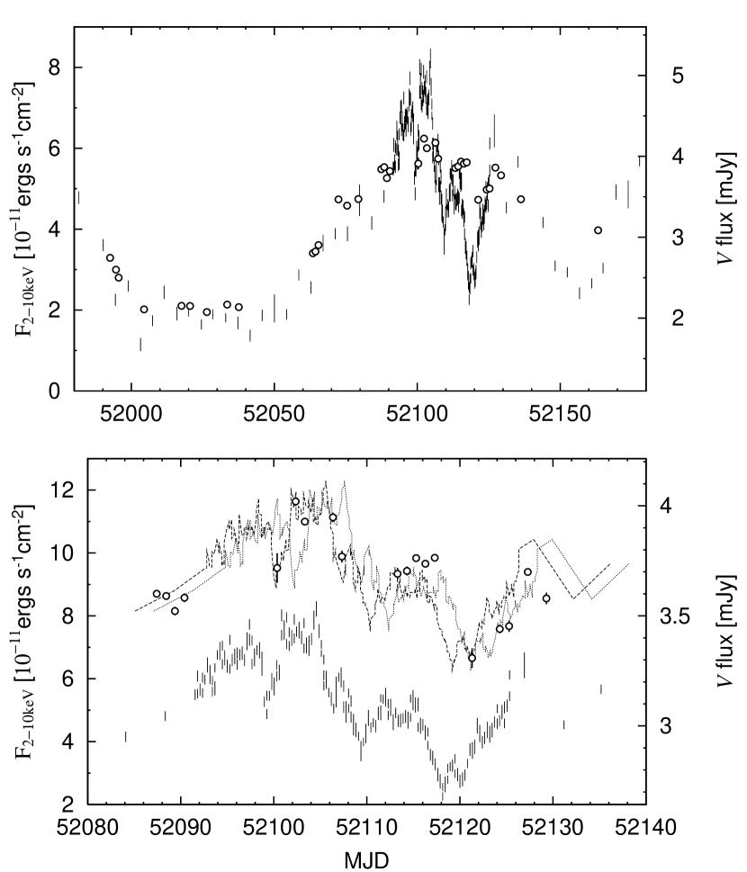
Figure 33: Top: Observed light curves of NGC 5548 in the $V$ band (open circles) and in the X-ray energy range of $2-10$ keV reported by Uttley et al. (2003). Bottom: Same as in the top panel, but only for the active phase in 2001 (${\rm MJD}\approx 52085-52130$) when the X-ray satellite (RXTE) observations were done intensively. The dashed line is the RXTE light curve shifted arbitrarily in the vertical direction and by $+1$ days in the horizontal direction, and the dotted line shifted by $+3$ days. Note that the scale for the optical flux is expanded in this panel.

The top panel of Figure 33 shows our $V$ light curve for NGC 5548 (Figure 8) and the X-ray ($2-10$ keV) light curve obtained for the same period from the Rossi X-ray Timing Explorer (RXTE, Uttley et al. 2003). These two light curves strongly correlate with each other, but the amplitude of the optical variation is much smaller than that of the X-ray. The bottom panel shows a portion of the light curves for a period of ${\rm MJD}\approx 52085-52130$ with an expanded vertical scale for the optical flux. Although the optical data were not sampled as often as the RXTE, a day-basis correlated variation as well as an optical lag of one day or two behind the X-ray is clearly seen. Cross-correlation analysis gives a lag time of $\Delta t=1.6_{-0.5}^{+1.0}$ days between the two light curves. A preliminary result was reported in Suganuma et al. (2004).

The size of the X-ray emitting region in AGNs is considered to be as small as a light-travel distance of hours, since a significant fraction of X-ray flux varies on this timescale (Figure 33). The observed correlated variability indicates that the optical emitting region in NGC 5548 is located at a light-travel distance of one day or two from the X-ray emitting region, and favors the thermal reprocessing of X-ray variability by the optically thick accretion disk, rather than a non-thermal process which emits both X-ray and UV/optical fluxes from almost the same region. On the other hand, the long-timescale X-ray and optical variations might be generated by some other mechanisms, such as instabilities of the accretion disk itself.

Our result also shows a geometrical relation between accretion disk and BLR. As seen in Figure 32, the broad emission line of highest ionization in NGC 5548 gives the shortest lag of a few days (Korista et al. 1995; Peterson & Wandel 1999). The detected lag time of one or two days indicates that the UV/optical emitting region of the accretion disk is located in the innermost part of the BLR in NGC 5548.

6 SUMMARY

We carried out the most intense monitoring observations yet made in optical and near-infrared wavebands for four nearby Seyfert 1 galaxies, including NGC 5548, NGC 4051, NGC 3227, and NGC 7469. Clear time-delayed response of the $K$-band flux variations to the $V$-band variations was detected for all the galaxies, which can be interpreted as light-travel time between the central engine and the inner edge of the dust torus. We modified a cross-correlation analysis to measure the lag times with high reliability, and our infrared lag times are found to range from 10 to 80 days, depending on the optical luminosity of the AGN. Comparing our infrared lag measurements with other quantities (optical luminosity, central virial mass, and broad-line lag) based on our sample and others in the literature, we summarize our findings as follows:

1. The infrared lag time is tightly correlated with the optical luminosity according to $\Delta t\propto L_{\rm opt}^{0.5}$ in agreement with the expected relation of dust reverberation.

2. A large scatter between lag time and central virial mass suggests that an inner radius of the dust torus is not directly related to the dynamics of a supermassive black hole at the center.

3. Infrared lags place an upper boundary on similar lag measurements of broad-emission lines in the literature. This not only supports the unified scheme of AGNs, but also implies a physical transition from the BLR out to the dust torus that encircles the BLR.

4. Our $V$ light curve for NGC 5548 shows a clear lag of one day or two behind the X-ray light curve obtained from the RXTE satellite, which indicates that the optical variation on short timescale originates in from the thermal reprocessing of X-rays by the optically thick accretion disk.

Ongoing monitoring observations for AGNs in our sample, aided by the results from other samples and different wavelengths, would enable us to understand the size and structure of dust torus of AGNs, not only from their statistical properties but also from their time evolution. Simultaneous reverberation studies of near-infrared continuum and broad emission lines of low ionization for several years would provide a clear view of the relation between dust torus and broad emission-line regions.

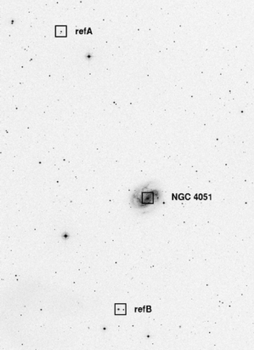
Figure 2: DSS $B_{j}$-band image of the photometric field for NGC 4051. The squares represent three $1^{\prime}.5\times 1^{\prime}.5$ fields of MIP camera. The left star (B1) in the ref B field is used for the $JK$ images, and the right star (B2) for the $BVH$ images.

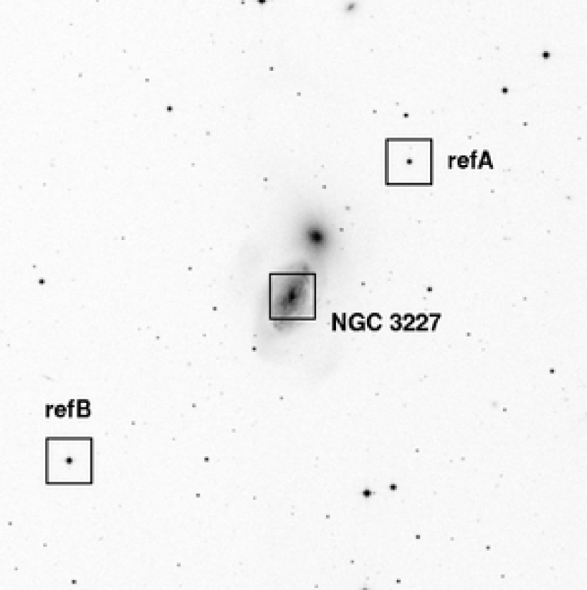
Figure 3: DSS $B_{j}$-band image of the photometric field for NGC 3227. The squares represent three $1^{\prime}.5\times 1^{\prime}.5$ fields of MIP camera.

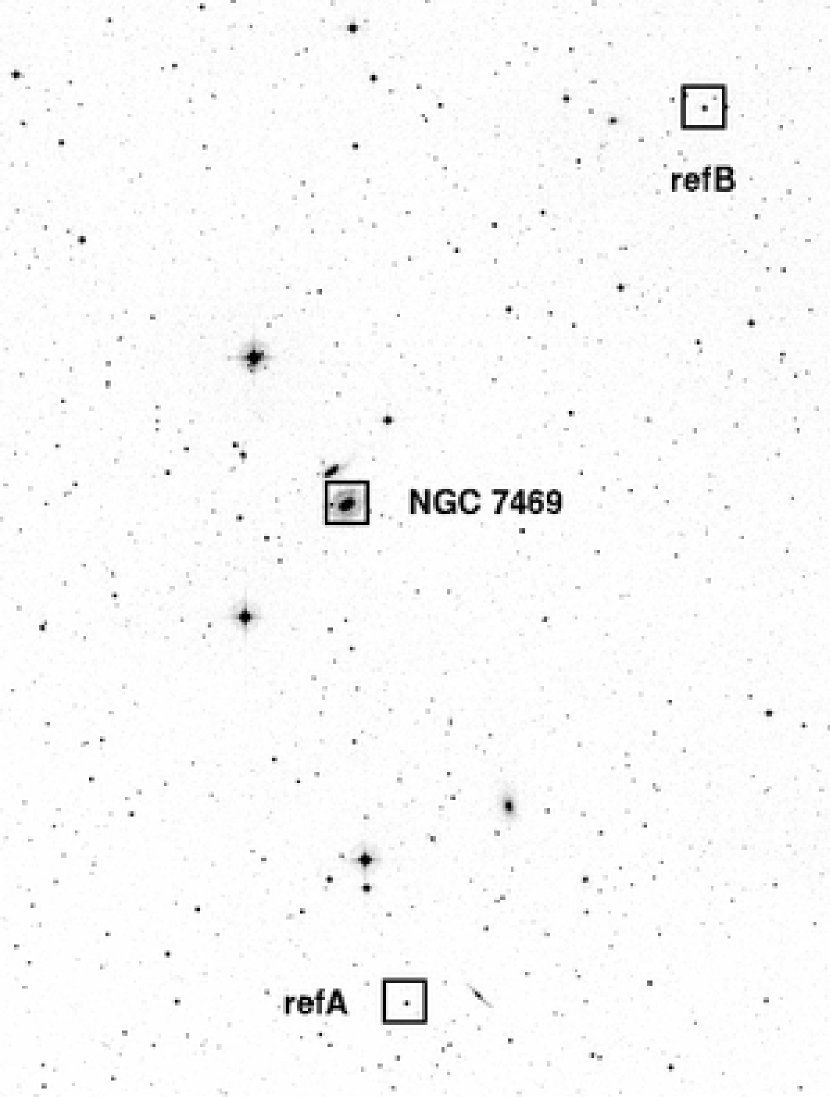
Figure 4: DSS $R$-band image of the photometric field for NGC 7469. The squares represent three $1^{\prime}.5\times 1^{\prime}.5$ fields of MIP camera.

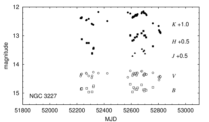
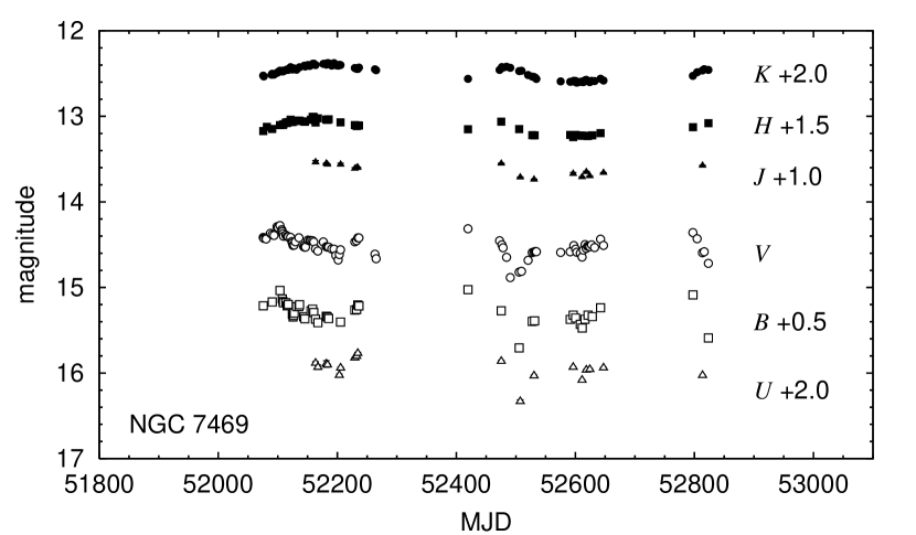
Figure 9: Observed $BVJHK$ light curves of NGC 3227 nucleus for the period from November 2001 to June 2003.

Figure 10: Observed $UBVJHK$ light curves of NGC 7469 nucleus for the period from June 2001 to July 2003.

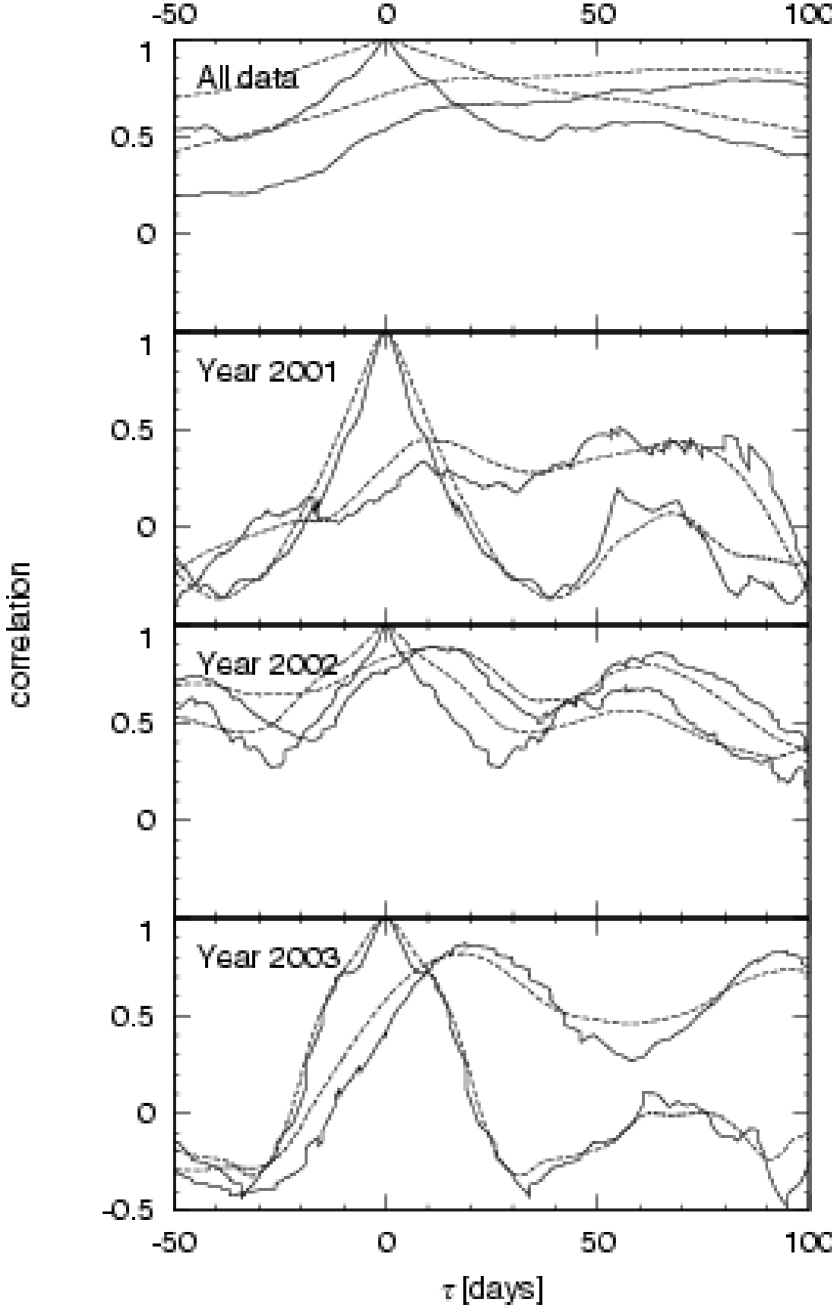
Figure 19: CCFs and ACFs for various monitoring periods. Same as Figure 18, but for NGC 4051. The CCFs are binodal with comparable peaks at $\tau_{\rm peak}=10-20$ days and $50-100$ days. We regard the mode of shorter $\tau_{\rm peak}$ as realistic one (see text).

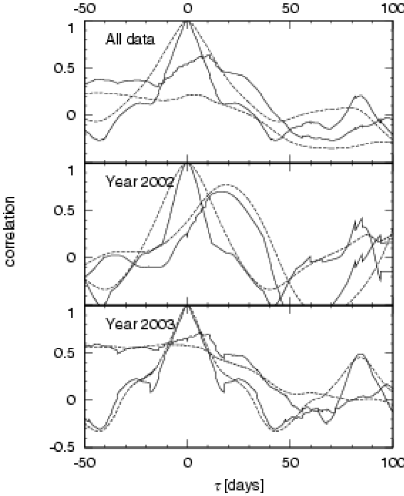
Figure 20: CCFs and ACFs for various monitoring periods. Same as Figure 18, but for NGC 3227. The CCFs on the top and bottom panels maintain a plateau level with no clear peak below $\tau\approx 5-10$ days.

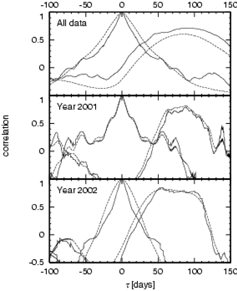
Figure 21: CCFs and ACFs for various monitoring periods. Same as Figure 18, but for NGC 7469.

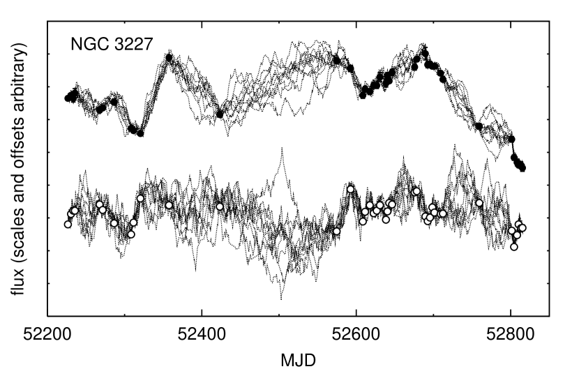
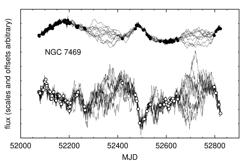
Figure 24: Simulated $V$ and $K$ light curves of NGC 3227. Others are the same as Figure 23.

Figure 25: Simulated $V$ and $K$ light curves of NGC 7469. Others are the same as Figure 23.

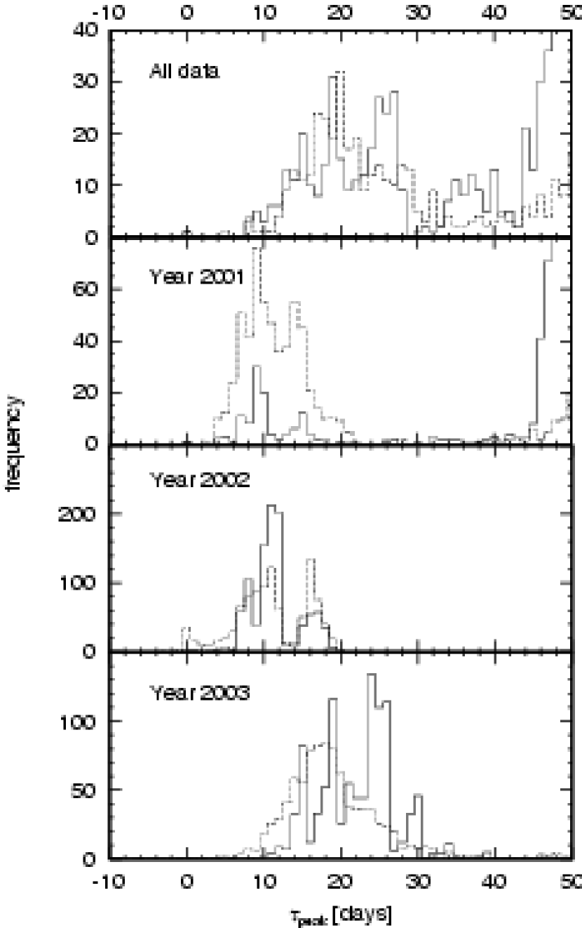
Figure 27: CCPDs for various monitoring periods. Same as Figure 26, but for NGC 4051. The lag time for the subset of all data as well as Year 2001 should be calculated from the histogram below $\tau_{\rm peak}\approx 42$ days (see text).

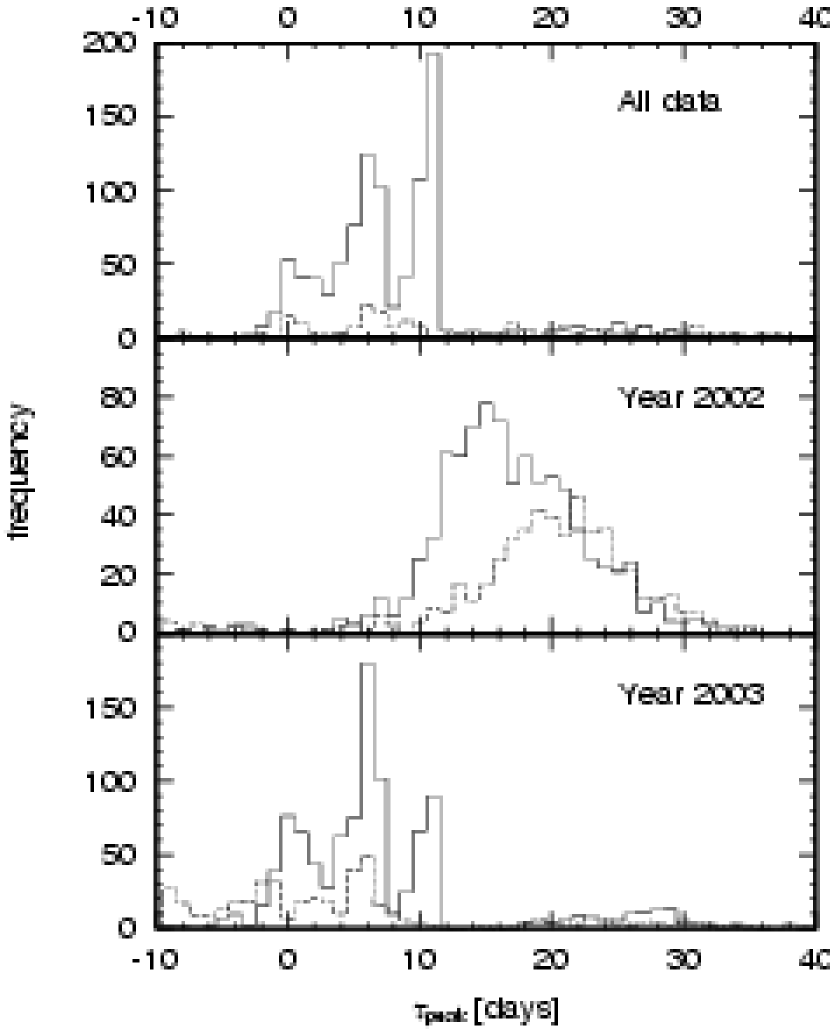
Figure 28: CCPDs for various monitoring periods. Same as Figure 26, but for NGC 3227.

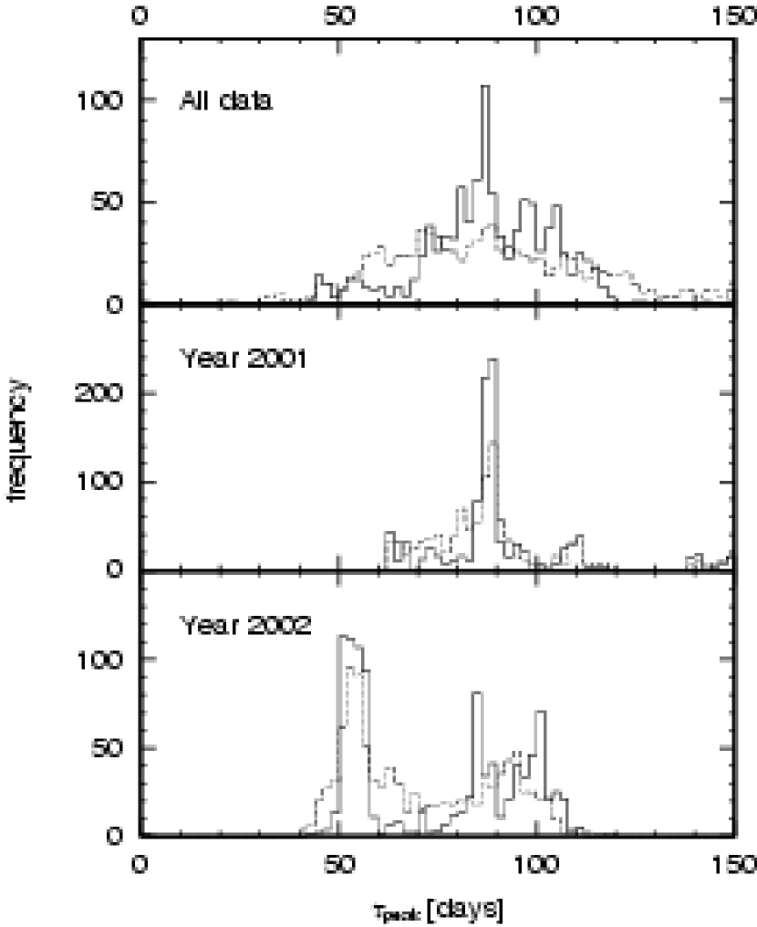
Figure 29: CCPDs for various monitoring periods. Same as Figure 26, but for NGC 7469.

Figure 30: Lag times between the UV/optical and $K$-band light curves of AGNs, plotted against the absolute $V$ magnitude. The filled symbols represent our results for NGC 5548 (squares), NGC 4051 (circles), NGC 3227 (triangle), and NGC 7469 (inverted triangles), including our earlier result for NGC 4151 (diamond, Minezaki et al. 2004). The others are data from the literature for Fairall 9 (pentagon, Clavel, Wamsteker & Glass 1989), GQ Comae (cross, Sitko et al. 1993), NGC 3783 (circle, Glass 1992), NGC 4151 (diamonds, Oknyanskij et al. 1999), and Mrk 744 (asterisk, Nelson 1996). Note that the horizontal bar in magnitude represents the observed range of flux variation during the observation.

Figure 31: Lag times for hot dust in Figure 30, plotted against the central virial mass estimated from the reverberation radii and widths of broad emission lines in individual AGNs (Peterson et al. 2004). Each symbol indicates the same AGN as in Figure 30. The inclined lines for various values of $c\Delta t/R_{g}$ are shown, where $R_{g}=2GM_{c}/c^{2}$ is the gravitational radius and $M_{c}$ is the central virial mass.

Figure 32: Lag times plotted against the absolute $V$ magnitude of AGNs. Filled and thick open symbols show the infrared lags, where each symbol indicates the same AGN as in Figure 30. Thin open symbols show the lag times of broad emission lines for the corresponding AGNs in the literature. Top: The lag times of only H$\beta$ line are plotted for broad emission lines. Bottom: The lag times of other broad lines are plotted.

Table 1: Characteristics of the target AGNs studied

Object	$\alpha$(2000)	$\delta$(2000)	$m_{V}$	$cz$	$A_{V}$	$M_{V}$
NGC5548 ……	$14^{\rm h}$ $17^{\rm m}$ $59^{\rm s}.5$	$+25^{\circ}$ $08^{{}^{\prime}}$ $12^{{}^{\prime\prime}}.4$	15.3	5359	0.068	$-19.2$
NGC4051 ……	$12^{\;\;}$ $03^{\;\;\>}$ $09^{\;}.6$	$+44^{\;\>}$ $31^{\;\>}$ $52^{\;\;}.8$	15.0	924	0.043	$-15.7$
NGC3227 ……	$10^{\;\;}$ $23^{\;\;\>}$ $30^{\;}.6$	$+19^{\;\>}$ $51^{\;\>}$ $54^{\;\;}.0$	14.4	1480	0.075	$-17.4$
NGC7469 ……	$23^{\;\;}$ $03^{\;\;\>}$ $15^{\;}.6$	$+08^{\;\>}$ $52^{\;\>}$ $26^{\;\;}.4$	14.5	4521	0.228	$-19.8$

Table 2: Apparent magnitudes of reference stars in the optical bands

Object	Star	$\alpha$(2000)	$\delta$(2000)	$U$ (mag)	$B$ (mag)			$V$ (mag)
NGC 5548	refA	$14^{\rm h}$ $17^{\rm m}$ $58^{\rm s}.9$	$+25^{\circ}$ $05^{{}^{\prime}}$ $34^{{}^{\prime\prime}}$	-	14.422	$\pm$	0.006 (19)	13.782	$\pm$	0.003 (37)
	refB1	$14^{\;\;}$ $17^{\;\;\>}$ $14^{\;\>}.7$	$+25^{\;\>}$ $19^{\;\>}$ $22^{\;\;}$	-	13.742	$\pm$	0.004 (19)	13.129	$\pm$	0.002 (37)
NGC 4051	refA	$12^{\;\;}$ $04^{\;\;\>}$ $13^{\;\>}.4$	$+44^{\;\>}$ $55^{\;\>}$ $03^{\;\;}$	-	13.568	$\pm$	0.007 (13)	12.636	$\pm$	0.003 (27)
	refB2	$12^{\;\;}$ $03^{\;\;\>}$ $30^{\;\>}.2$	$+44^{\;\>}$ $16^{\;\>}$ $46^{\;\;}$	-	14.472	$\pm$	0.005 (13)	13.874	$\pm$	0.006 (27)
NGC 3227	refA	$10^{\;\;}$ $23^{\;\;\>}$ $13^{\;\>}.6$	$+19^{\;\>}$ $56^{\;\>}$ $25^{\;\;}$	-	13.394	$\pm$	0.003 ( 7)	12.771	$\pm$	0.003 (12)
	refB	$10^{\;\;}$ $24^{\;\;\>}$ $02^{\;\>}.9$	$+19^{\;\>}$ $46^{\;\>}$ $31^{\;\;}$	-	12.506	$\pm$	0.003 ( 7)	11.959	$\pm$	0.003 (12)
NGC 7469	refA	$23^{\;\;}$ $03^{\;\;\>}$ $07^{\;\>}.1$	$+08^{\;\>}$ $34^{\;\>}$ $30^{\;\;}$	14.21$\pm$0.01 (6)	13.918	$\pm$	0.003 ( 4)	13.180	$\pm$	0.003 (18)
	refB	$23^{\;\;}$ $02^{\;\;\>}$ $23^{\;\>}.4$	$+09^{\;\>}$ $06^{\;\>}$ $41^{\;\;}$	14.43$\pm$0.01 (6)	13.891	$\pm$	0.003 ( 4)	12.998	$\pm$	0.003 (18)

Note. — The number of photometric calibrations for each star and band is given in the parentheses.

Table 3: Apparent magnitudes of reference stars in the near-infrared bands

Object	Star	$\alpha$(2000)	$\delta$(2000)	$J$ (mag)				$H$ (mag)				$K$ (mag)
NGC 5548	refA	$14^{\rm h}$ $17^{\rm m}$ $58^{\rm s}.9$	$+25^{\circ}$ $05^{{}^{\prime}}$ $34^{{}^{\prime\prime}}$		-			12.227	$\pm$	0.004	(3)	12.196	$\pm$	0.006 ( 9)
	refB1	$14^{\;\;}$ $17^{\;\;\>}$ $14^{\;\>}.7$	$+25^{\;\>}$ $19^{\;\>}$ $22^{\;\;}$		-				-			11.531	$\pm$	0.004 ( 9)
	refB2	$14^{\;\;}$ $17^{\;\;\>}$ $12^{\;\>}.2$	$+25^{\;\>}$ $19^{\;\>}$ $33^{\;\;}$		-			13.072	$\pm$	0.009	(3)		-
NGC 4051	refA	$12^{\;\;}$ $04^{\;\;\>}$ $13^{\;\>}.4$	$+44^{\;\>}$ $55^{\;\>}$ $03^{\;\;}$	10.606	$\pm$	0.004	(4)	10.06	$\pm$	0.01	(1)	9.948	$\pm$	0.004 (13)
	refB1	$12^{\;\;}$ $03^{\;\;\>}$ $34^{\;\>}.0$	$+44^{\;\>}$ $16^{\;\>}$ $50^{\;\;}$	10.545	$\pm$	0.004	(4)		-			10.243	$\pm$	0.003 (13)
	refB2	$12^{\;\;}$ $03^{\;\;\>}$ $30^{\;\>}.2$	$+44^{\;\>}$ $16^{\;\>}$ $46^{\;\;}$		-			12.34	$\pm$	0.01	(1)		-
NGC 3227	refA	$10^{\;\;}$ $23^{\;\;\>}$ $13^{\;\>}.6$	$+19^{\;\>}$ $56^{\;\>}$ $25^{\;\;}$	11.483	$\pm$	0.005	(5)	11.143	$\pm$	0.004	(9)	11.092	$\pm$	0.004 (13)
	refB	$10^{\;\;}$ $24^{\;\;\>}$ $02^{\;\>}.9$	$+19^{\;\>}$ $46^{\;\>}$ $31^{\;\;}$	10.806	$\pm$	0.005	(5)	10.508	$\pm$	0.004	(9)	10.459	$\pm$	0.004 (13)
NGC 7469	refA	$23^{\;\;}$ $03^{\;\;\>}$ $07^{\;\>}.1$	$+08^{\;\>}$ $34^{\;\>}$ $30^{\;\;}$	11.74	$\pm$	0.01	(2)	11.366	$\pm$	0.010	(4)	11.308	$\pm$	0.006 ( 9)
	refB	$23^{\;\;}$ $02^{\;\;\>}$ $23^{\;\>}.4$	$+09^{\;\>}$ $06^{\;\>}$ $41^{\;\;}$	11.22	$\pm$	0.01	(2)	10.778	$\pm$	0.010	(4)	10.696	$\pm$	0.004 ( 9)

Note. — The number of photometric calibrations for each star and band is given in the parentheses. The uncertainties of the photometric standard stars, typically about 0.01 mag, are not included in the calibrations.

Table 4: Host galaxy flux in the $\phi=8^{\prime\prime}.3$ aperture

Object	$U$	$B$	$V$	$J$	$H$	$K$
NGC 5548 ……	-	1.4	3.7	-	20	16
NGC 4051 ……	-	4.7	8.6	41	47	39
NGC 3227 ……	-	3.0	6.4	50	66	60
NGC 7469 ……	3.3	5.4	8.6	41	54	56

Table 5: Coefficients for seeing correction in equation 1

Object	Band	$b$			$c$
NGC 5548 ……	$B$	$-$0	.	025	0	.	058
	$V$	0	.	001	0	.	095
	$H$	0	.	23	0	.	28
	$K$	0	.	41		-
NGC 4051 ……	$V$	$-$0	.	02	0	.	066
	$K$	0	.	006	0	.	39
NGC 7469 ……	$U$	0	.	058		-
	$B$	$-$0	.	007	0	.	066
	$V$	0	.	066	0	.	075
	$J$	0	.	77		-
	$H$	0	.	54	0	.	81
	$K$	0	.	67	0	.	55

Note. — No seeing correction was attempted in the cases of $BJH$ for NGC 4051 and $BVJHK$ for NGC 3227, because of larger photometric errors.

Table 6: Sampling statistics for the $V$ and $K$ bands

			$V$ Band				$K$ Band
Object	Span	$\Delta T_{\rm max}$	$N$	$\Delta T_{\rm ave}$	$\Delta T_{\rm med}$		$N$	$\Delta T_{\rm ave}$	$\Delta T_{\rm med}$
NGC 5548 ……	893	110	101	8.9	3		95	9.5	4
NGC 4051 ……	915	112	84	11.0	5		89	10.4	5
NGC 3227 ……	589	151	40	15.1	4		40	15.1	4
NGC 7469 ……	748	154	88	8.6	3		86	8.8	3

Note. — $N$ is the number of data points, and others are various time intervals in units of days.

Table 7: Variability statistics in the $V$ and $K$ bands

	$V$ Band					$K$ Band
Object	$\left<f\right>$	$\sigma$	$F_{\rm var}$	$R_{\rm max}$		$\left<f\right>$	$\sigma$	$F_{\rm var}$	$R_{\rm max}$
NGC 5548 ……	2.6	0.9	0.32	3.2		16	4	0.26	2.9
NGC 4051 ……	3.6	0.6	0.16	2.0		31	7	0.22	2.5
NGC 3227 ……	6.6	0.4	0.06	1.3		18	3	0.18	2.0
NGC 7469 ……	5.8	0.6	0.10	1.8		41	3	0.06	1.2

Note. — $\left<f\right>$ is the mean flux, and $\sigma$ is the rms variation in units of mJy. $F_{\rm var}$ is the normalized variability amplitude defined in equation 2, and $R_{\rm max}$ is the ratio of maximum to minimum fluxes defined as $f_{{\rm max}}/f_{{\rm min}}$.

Table 8: Cross-correlation results from the observed light curves

				BI Method				ES Method
Object	Subset	MJD	$N$	$\tau_{\rm peak}$		$r_{\rm max}$		$\tau_{\rm peak}$		$r_{\rm max}$
NGC 5548 ……	All data	$51992-52885$	101	45	.1	0.909		49	.2	0.920
	Year 2001	$51992-52163$	36	47	.8	0.962		48	.0	0.961
	Year 2002-2003	$52265-52823$	52	49	.5	0.968		48	.3	0.947
	Year 2003	$52622-52885$	42	57	.0	0.952		53	.1	0.946
NGC 4051 ……	All data	$51917-52819$	84	$>$5	0	-		$>$5	0	-
	Year 2001	$51917-52117$	28	9	.0	0.347		10	.3	0.479
	Year 2002	$52229-52488$	30	11	.3	0.894		11	.4	0.886
	Year 2003	$52599-52819$	26	25	.9	0.804		17	.7	0.779
NGC 3227 ……	All data	$52226-52815$	40	10	.9	0.640		$<$8		-
	Year 2002	$52226-52423$	12	16	.7	0.701		18	.9	0.772
	Year 2003	$52574-52815$	28	6	.7	0.714		$<$5		-
NGC 7469 ……	All data	$52075-52647$	88	87	.7	0.716		86	.0	0.606
	Year 2001	$52075-52265$	53	88	.8	0.798		87	.9	0.822
	Year 2002	$52419-52647$	30	52	.9	0.846		55	.4	0.826

Note. — $N$ is the number of data points. $\tau_{\rm peak}$ is the position at which the CCF peak occurs, and $r_{\rm max}$ is the peak value of CCF.

Table 9: Structure functions from the observed light curves

	$V$ Band				$K$ Band
Object	$S_{0}$	$\beta$	$\tau_{\rm max}$		$S_{0}$	$\beta$	$\tau_{\rm max}$
NGC 5548 ……	$1.8\times 10^{-3}$	1.46	60		$1.7\times 10^{-3}$	$2.0$	60
NGC 4051 ……	$2.4\times 10^{-2}$	0.71	30		$7.9\times 10^{-2}$	$1.5$	30
NGC 3227 ……	$2.1\times 10^{-2}$	0.91	20		$4.0\times 10^{-2}$	$1.1$	50
NGC 7469 ……	$3.2\times 10^{-2}$	0.82	30		$1.6\times 10^{-2}$	$1.6$	50

Note. — $S_{0}$ is the fiducial flux in units of $({\rm mJy})^{2}$ at time interval of one day, $\beta$ is the power-law index of structure function, and $\tau_{\rm max}$ is the upper bound of days for power-law fit.

Table 10: Cross-correlation results from the simulated light curves

Object	Subset	$M_{V}$	Magnitude Range		Lag Time (BI)			Lag Time (ES)
NGC 5548 ……	All data	$-19.19$	$[-18.39,\;-19.65\;]$			$45.1$	${}_{-3.4}^{+1.5}$		$48.7$	${}_{-4.1}^{+4.6}$
	Year 2001	$-19.39$	$[-18.88,\;-19.65\;]$			$47.8$	${}_{-1.2}^{+1.7}$		$48.0$	${}_{-2.3}^{+2.7}$
	Year 2002-2003	$-19.04$	$[-18.39,\;-19.60\;]$			$47.3$	${}_{-5.6}^{+3.9}$		$46.7$	${}_{-5.3}^{+4.8}$
	Year 2003	$-19.18$	$[-18.39,\;-19.60\;]$			$57.0$	${}_{-6.2}^{+1.2}$		$52.9$	${}_{-5.8}^{+3.0}$
NGC 4051 ……	All data	$-15.65$	$[-15.27,\;-16.02\;]$			$24.1$	${}_{-9.2}^{+11.1}$		$21.0$	${}_{-4.8}^{+8.4}$
	Year 2001	$-15.51$	$[-15.27,\;-15.76\;]$			$10.2$	${}_{-2.2}^{+16.4}$		$10.9$	${}_{-3.7}^{+4.2}$
	Year 2002	$-15.66$	$[-15.38,\;-16.02\;]$			$11.0$	${}_{-2.9}^{+4.4}$		$10.8$	${}_{-4.0}^{+5.5}$
	Year 2003	$-15.77$	$[-15.56,\;-16.02\;]$			$22.8$	${}_{-5.9}^{+3.1}$		$18.1$	${}_{-4.4}^{+6.2}$
NGC 3227 ……	All data	$-17.35$	$[-17.15,\;-17.47\;]$			$6.8$	${}_{-4.6}^{+4.1}$		-
	Year 2002	$-17.35$	$[-17.23,\;-17.43\;]$			$16.3$	${}_{-4.4}^{+6.0}$		$20.2$	${}_{-5.7}^{+5.2}$
	Year 2003	$-17.35$	$[-17.15,\;-17.47\;]$			$6.0$	${}_{-5.4}^{+4.8}$		-
NGC 7469 ……	All data	$-19.78$	$[-19.40,\;-20.00\;]$			$87.6$	${}_{-14.3}^{+16.7}$		$85.4$	${}_{-24.3}^{+26.7}$
	Year 2001	$-19.82$	$[-19.60,\;-20.00\;]$			$88.0$	${}_{-8.4}^{+17.8}$		$86.9$	${}_{-14.1}^{+17.5}$
	Year 2002	$-19.71$	$[-19.39,\;-19.96\;]$			$77.7$	${}_{-25.5}^{+21.7}$		$64.9$	${}_{-12.8}^{+29.4}$

Note. — $M_{V}$ is the absolute $V$-band magnitude averaged over the magnitude range observed. The lag time is a median of $\tau_{\rm peak}$ in the CCPD. For NGC 3227, when the CCPD results in too broad a distribution, reflecting the plateau feature in the CCF (Figure 20), the lag time is given no value in the blank column.

References

- (1) Antonucci, R. 1993, ARA&A, 31, 473
- (2) Barvainis, R. 1987, ApJ, 320, 537
- (3) Barvainis, R. 1992, ApJ, 400, 502
- (4) Clavel, J., Wamsteker, W., & Glass, I. S. 1989, ApJ, 337, 236
- (5) Clavel, J. et al. 1990, MNRAS, 246, 668
- (6) Clavel, J. et al. 1992, ApJ, 393, 113
- (7) Collier, S., et al. 1998, ApJ, 500, 162
- (8) Collin-Souffrin, S. et al. 1991, A&A, 249, 344
- (9) Dietrich, M. et al. 1993, ApJ, 408, 416
- (10) Frank, J., King, A. R., & Raine, D. J. 1992, Accretion Power in Astrophysics (2d ed.; Cambridge: Cambridge Univ. Press)
- (11) Gaskell, C. M., & Peterson, B. M. 1987, ApJS, 65, 1
- (12) Glass, I. S. 1992, MNRAS, 256, 23P
- (13) Glass, I. S. 2004, MNRAS, 350, 1049
- (14) Hayashida, K., Miyamoto, S., Kitamoto, S., Negoro, H. 1998, ApJ, 500, 642
- (15) Hunt, L. K., Mannucci, F., Testi, L., Migliorini, S., Stanga, R. M., Baffa, C., Lisi, F., & Vanzi, L. 1998, AJ, 115, 2594
- (16) Kaspi, S. et al. 1996, ApJ, 470, 336
- (17) Kaspi, A., Smith, P. S., Netzer, H., Maoz, D., Jannuzi, B. T., & Giveon, U. 2000, ApJ, 533, 631
- (18) Kobayashi, Y., Sato, S., Yamashita, T., Shibai, H., Takami, H., 1993, ApJ, 404, 94
- (19) Kobayashi, Y. et al. 1998a, Proc. SPIE, 3352, 120
- (20) Kobayashi, Y., Yoshii, Y., Peterson, B. A., Minezaki, T., Enya, K., Suganuma, M., & Yamamuro, T. 1998b, Proc. SPIE, 3354, 769
- (21) Kobayashi, Y. et al. 2003, Proc. SPIE, 4837, 954
- (22) Korista, K. T. et al. 1995, ApJS, 97, 285
- (23) Kriss, G. A., Peterson, B. M., Crenshaw, D. M., & Zheng, W. 2000, ApJ, 535, 58
- (24) Krolik, J. H., Horne, K., Kallman, T. R., Malkan, M. A., Edelson, R. A., & Kriss, G. A. 1991, ApJ, 371, 541
- (25) Landolt, A. U. 1992, AJ, 104, 340
- (26) Maoz, D. & Netzer, H. 1989, MNRAS, 236, 21
- (27) Maoz, D. et al. 1991, ApJ, 367, 493
- (28) Minezaki, T., Yoshii, Y., Kobayashi, Y., Enya, K., Suganuma, M., Tomita, H., Aoki, T., & Peterson, B. A. 2004, ApJ, 600, L35
- (29) Nelson, B. O. 1996, ApJ, 465, L87
- (30) Netzer, H. & Laor, A. 1993, ApJ, 404, L51
- (31) Oknyanskij, V. L., Lyuty, V. M., Taranova, O. G., & Shenavrin, V. I. 1999, Astronomy Letters, 25, 483
- (32) Onken, C. A., Peterson, B. M., Dietrich, M., Robinson, A., & Salamanca, I. M. 2003, ApJ, 585, 121
- (33) Peng, C. Y., Ho, L. C., Impey, C. D., & Rix, H.-W. 2002, AJ, 124, 266
- (34) Peterson, B. M. 1993, PASP, 105, 247
- (35) Peterson, B. M. 2001, in Advanced Lectures on the Starburst-AGN Connection, ed. I. Aretxaga, D. Kunth, & R. Mújica (Singapore: World Scientific), 3
- (36) Peterson, B. M., Wanders, I., Horne, K., Collier, S., Alexander, T., Kaspi, S., & Maoz, D. 1998, PASP, 110, 660
- (37) Peterson, B. M. & Wandel, A. 1999, ApJ, 521, L95
- (38) Peterson, B. M. et al. 2002, ApJ, 581, 197
- (39) Peterson, B. M. et al. 2004, ApJ, 613, 682
- (40) Reichert, G. A. et al. 1994, ApJ, 425, 582
- (41) Rodriguez-Pascual, P. M. et al. 1997, ApJS, 110, 9
- (42) Shemmer, O., Uttley, P., Netzer, H., & McHardy, I. M. 2003, MNRAS, 343, 1341
- (43) Simonetti, J. H., Cordes, J. M., & Heeschen, D. S. 1985, ApJ, 296, 46
- (44) Sitko, M. L., Sitko, A. K., Siemiginowska, A., & Szczerba, R. 1993, ApJ, 409, 139
- (45) Suganuma, M. et al. 2004, ApJ, 612, L113
- (46) Uttley, P., McHardy, I. M., Papadakis, I. E. 2002, MNRAS, 332, 231
- (47) Uttley, P., McHardy, I. M., Peterson, B. M., & Markowitz, A. 2003, ApJ, 584, L53
- (48) Wandel, A., Peterson, B. M., & Malkan, M. A. 1999, ApJ, 526, 579
- (49) Wanders, I., et al. 1997, ApJS, 113, 69
- (50) White, R. J. & Peterson, B. M. 1994, PASP, 106, 879
- (51) Winge, C., Peterson, B. M., Horne, K., Pogge, R. W., Pastoriza, M. G., & Storchi-Bergmann, T. 1995, ApJ, 445, 680
- (52) Winkler, H., Glass, I. S., Wyk, F. van, Marang, F., Spencer Jones, J. H., Buckley, D. A. H., Sekiguchi, K. 1992, MNRAS, 257, 659
- (53) Winkler, H. 1997, MNRAS, 292, 273
- (54) Yoshii, Y. 2002, in New Trends in Theoretical and Observational Cosmology, ed. K. Sato and T. Shiromizu (Tokyo: Universal Academy Press), 235