Combining weak and strong lensing in cluster potential reconstruction

We propose a method for recovering the two-dimensional gravitational potential of galaxy clusters which combines data from weak and strong gravitational lensing. A first estimate of the potential from weak lensing is improved at the approximate locations of critical curves. The method can be fully linearised and does not rely on the existence and identification of multiple images. We use simulations to show that it recovers the surface-mass density profiles and distributions very accurately,even if critical curves are only partially known and if their location is realistically uncertain. We further describe how arcs at different redshifts can be combined, and how deviations from weak lensing can be included.

1 Introduction

Weak gravitational lensing constrains the projected mass distributions of galaxy clusters with an angular resolution of $\gtrsim 0.5^{\prime}$, while strong lensing occurs typically not farther than $(0.5-1)^{\prime}$ from cluster cores. Nonetheless, both phenomena are due to the same gravitational potential. Recent observations of galaxy clusters with the ACS camera on-board HST (see Broadhurst et al. 2005 for an example) have revealed large numbers of arcs in individual galaxy clusters, for which Abell 1689 is an outstanding example. In such clusters, strongly lensed images provide numerous constraints on the lensing potential, and the question is raised how weak and strong lensing are best combined in joint reconstructions of the lensing mass distribution.

Several methods were recently proposed which rely on the identification of multiply-imaged systems (Bradač et al., 2005a, b; Diego et al., 2005). We propose an alternative method here for which multiple images are not necessary and thus do not need to be identified. Based on a least-$\chi^{2}$ minimisation, a first estimate of the lensing potential is obtained from weak lensing alone, following the approach suggested by Bartelmann et al. (1996) and Seitz et al. (1998). Where the position of critical curves can be approximately identified due to the presence of strongly-lensed images, this estimate is improved by requiring that the determinant of the Jacobian matrix vanish. The method is easily generalised to sources at different redshifts. It can be fully linearised and allows deviations from the strict weak-lensing limit to be accounted for by simple iteration.

We outline the main ideas underlying the method in Sect. 2. After reviewing the necessary formalism of gravitational lensing in Sect. 3, we describe the method in Sect. 4 and illustrate its feasibility using numerical simulations in Sect. 5. Conclusions are given in Sect. 6, and technical detail is summarised in the Appendix.

2 Overview

The method we are proposing rests on two central ideas. First, both weak and strong lensing must be described by the same underlying, two-dimensional lensing potential. Data from weak and strong lensing observations must thus be expressed in terms of constraints on the potential. Second, strong lensing can be located in several ways, of which the identification of multiple images is one, and the existence of critical curves is another. Recent images of strongly-lensing galaxy clusters illustrate that gravitational arcs in many cases allow an accurate, piece-wise localisation of critical curves. On the other hand, multiple images need to be identified first and are only caused by sources close to and inside caustics, while sources outside caustics can still be used to identify critical curves.

Based on these ideas, our algorithm can be summarised very simply: we wish to find a map of the lensing potential, discretised on a grid, which is determined such as to optimise the agreement with the observed data. The gravitational shear caused by weak lensing imprints coherent distortions on the images of background galaxies. To lowest-order approximation, their average ellipticity is an unbiased estimator of the local shear. The lensing potential must be arranged such as to reproduce this measured shear. Critical curves occur at singular points of the lens mapping, which locally constrain the curvature matrix of the potential. Thus, our algorithm aims at optimally constraining the potential such that its tidal field reproduces the measured shear, and its curvature reproduces the critical curves.

Several complications come to mind immediately. First, there is a problem of scales. Given number densities of $\sim 30-40$ background galaxies per square arc minute, the angular resolution of weak-lensing observations is limited to $\gtrsim 0.5^{\prime}$. Strong lensing, however, typically happens within $\lesssim 1^{\prime}$ of cluster centres. Both can be combined only if grids of high resolution in the core and low resolution farther outside are used. For the practical implementation, we choose to first reconstruct the potential at low resolution on a coarse grid, then refine the grid everywhere in the core area where critical curves exist, fill the refined grid by suitable interpolation from the coarse grid, and correct the potential there such as to reproduce the critical curves.

Second, galaxy ellipticities reflect the shear $\gamma$ only in the limit of weak lensing, $\kappa\ll 1$. Deviations occur towards critical curves. Outside critical curves, ellipticities constrain the reduced shear $\gamma/(1-\kappa)$, and its inverse complex conjugate $1/g^{*}$ inside. As other studies (e.g. Bradač et al. (2005b)) have remarked earlier, this is not a problem of principle because it can be solved in a quickly converging iteration.

Third, arcs in clusters typically originate from sources at different redshifts. Since the geometrical efficiency of a fixed lens increases monotonically with source redshift, so does the lensing potential. Arcs at different redshifts thus constrain the curvature of a lensing potential with the same shape but different amplitude. However, the potential grows with source redshift by a linear factor. This suggests the introduction of a reference potential for one arbitrary source redshift, to which the potentials for sources at other redshifts can linearly be transformed.

Fourth, critical curves can almost never be traced throughout a cluster, but only piece-wise. This is irrelevant for our purposes since the constraint that the curvature of the lensing potential must reproduce the critical curves is purely local. As the distortion of arcs close to critical curves varies rapidly with position, measurement errors for the location of critical curves are typically small. Alternatively, constraints on critical curves obtained from parameterised lens models can be used in a hybrid approach.

Finally, all constraints can be expressed in terms of second derivatives of the lensing potential. In the limit of weak lensing, the constraints are linear since the source ellipticity is then a linear combination of second potential derivatives. Moving into the strong-lensing regime, the ellipticity constraints can be kept linear by means of an iterative procedure. We devise a scheme in which even the constraints from critical curves can be expressed by a linear correction term. While this linearity is not conceptually important, it is practically because it allows minimisations by matrix inversions.

3 Basic formalism

We start by reviewing the basic formalism for gravitational lensing as we shall need it in the course of the paper. Dealing with isolated lensing systems such as galaxy clusters, we adopt the thin-lens approximation, according to which the lensing mass distribution is projected onto a lens plane perpendicular to the line-of-sight. Sources are located on source planes which are also perpendicular to the line-of-sight. The lens system is characterised by the three angular-diameter distances $D_{\mathrm{l,s,ls}}$ between the observer and the lens, the observer and the source, and between lens and source, respectively.

All relevant properties of the lens system are then contained in the scalar lensing potential $\psi$, which is the suitably projected and rescaled Newtonian gravitational potential $\Phi$ of the lens,

$$\psi(\@vec{\theta})=\frac{2}{c^{2}}\frac{D_{\mathrm{ls}}}{D_{\mathrm{l}}D_{\mathrm{s}}}\,\int\Phi(D_{\mathrm{l}}\@vec{\theta})\,\mathrm{d}z$$ (1)

(e.g. Schneider et al. 1992). Obviously, the lensing potential depends on the source redshift. Assuming that the lensing mass distribution is the same for sources on different source planes, we can still introduce a single scalar potential $\bar{\psi}(\@vec{\theta})$ for a fiducial source redshift $\bar{z}_{\mathrm{s}}$, and then scale the potential to other source redshifts $z_{\mathrm{s}}$ according to

$$\psi(\@vec{\theta},z_{\mathrm{s}})=\bar{\psi}(\@vec{\theta})\,\frac{D_{\mathrm{ls}}(z_{\mathrm{s}})}{D_{\mathrm{s}}(z_{\mathrm{s}})}\frac{D_{\mathrm{s}}(\bar{z}_{\mathrm{s}})}{D_{\mathrm{ls}}(\bar{z}_{\mathrm{s}})}\;.$$ (2)

The linearity of this transformation allows the linear reconstruction of the single, fiducial lensing potential $\bar{\psi}$ from sources on multiple source planes.

The two-dimensional, projected mass distribution of the lens is described by the convergence $\kappa$, which is the surface mass density $\Sigma$ in units of

$$\Sigma_{\mathrm{cr}}=\left(\frac{4\pi G}{c^{2}}\frac{D_{\mathrm{l}}D_{\mathrm{ls}}}{D_{\mathrm{s}}}\right)^{-1}\;.$$ (3)

Distortions caused by the lens are characterised by the trace-free, symmetric shear tensor with the two components $\gamma_{1,2}$. Both are linear combinations of second derivatives of $\psi$,

$$\gamma_{1}=\frac{1}{2}\left(\psi,_{11}-\psi,_{22}\right)\;,\quad\gamma_{2}=\psi,_{12}\;,\quad\kappa=\frac{1}{2}\@vec{\nabla}^{2}\psi\;.$$ (4)

The lens mapping relates the source position $\@vec{\beta}$ to the image position(s) $\@vec{\theta}$,

$$\@vec{\beta}=\@vec{\theta}-\@vec{\nabla}\psi(\@vec{\theta})\;.$$ (5)

For sources which are small compared to typical scales of the (reduced) deflection angle $\@vec{\alpha}=\@vec{\nabla}\psi$, the lens mapping can be linearised. Imaging is then locally characterised by the Jacobian matrix

$$\mathcal{A}=\frac{\partial\@vec{\beta}}{\partial\@vec{\theta}}=\left(\begin{array}[]{cc}1-\kappa-\gamma_{1}&-\gamma_{2}\\ -\gamma_{2}&1-\kappa+\gamma_{1}\\ \end{array}\right)\ .$$ (6)

This shows that $\kappa$ is responsible for shrinking or stretching images isotropically, while $\gamma$ causes anisotropic deformation.

A sufficiently small circular source of radius $r$ is imaged as an ellipse with semi-major and -minor axes $a=r(1-\kappa-\gamma)^{-1}$ and $b=r(1-\kappa+\gamma)^{-1}$, respectively. The ellipticity, defined as $\epsilon\equiv(a-b)/(a+b)$, is thus

$$\epsilon=\frac{\gamma}{1-\kappa}\equiv g\;,$$ (7)

defining the so-called reduced shear $g$. In the weak-lensing regime, characterised by $\kappa\ll 1$ and $\gamma_{1,2}\ll 1$, the ellipticity approximates the shear, $\epsilon\approx\gamma$. In gravitational lenses capable of strong lensing, the weak-lensing approximation typically fails very close to the centre. While the linear relation between ellipticity and shear can then be applied in the outskirts of the lens, corrections may become necessary near the core.

Critical curves $\@vec{\theta}_{\mathrm{c}}$ are closed curves in the lens plane consisting of points where $\mathcal{A}$ cannot be inverted, $\det\mathcal{A}(\@vec{\theta}_{\mathrm{c}})=0$. Their images in the source plane under the lens mapping (5) are called caustics; they are given by $\@vec{\beta}_{\mathrm{c}}=\@vec{\theta}_{\mathrm{c}}-\@vec{\nabla}\psi(\@vec{\theta}_{\mathrm{c}})$. Obviously, the relation

$$(1-\kappa)^{2}-|\gamma|^{2}=0$$ (8)

is satisfied along critical curves.

Any measurement of gravitational lensing which is based on local distortion information alone cannot distinguish between lensing with the Jacobian matrices $\mathcal{A}$ and $\lambda\mathcal{A}$, with $\lambda\neq 0$. The matrix $\lambda\mathcal{A}$ produces images which are isotropically stretched by the factor $\lambda$, but with identical ellipticity $\epsilon$ as the matrix $\mathcal{A}$. This invariance against the transformation $\mathcal{A}\to\lambda\mathcal{A}$ causes $\kappa$ and $\gamma$ to be invariant against the transformation

$$\kappa\to(1-\lambda)+\lambda\kappa\;,\quad\gamma\to\lambda\gamma\;,$$ (9)

which obviously leaves the reduced shear (7) invariant. This invariance transformation was first described as a “mass-sheet degeneracy” (Falco et al. 1985; Schneider & Seitz 1995) because it tends to $\kappa\to(1-\lambda)+\kappa$ in the limit of $|1-\lambda|\to 0$.

We emphasise in the context of our joint reconstruction method that the critical curves are also invariant under the transformation (9). Obviously, the defining condition $\det\mathcal{A}=0$ for critical curves is unchanged if $\mathcal{A}$ is multiplied by $\lambda\neq 0$. Translated to the underlying lensing potential, the transformation (9) allows transformations of the potential of the form

$$\psi\to\lambda\psi+\frac{1-\lambda}{2}(\theta_{1}^{2}+\theta_{2}^{2})+a\theta_{1}+b\theta_{2}+c\;,$$ (10)

with arbitrary constants $a$, $b$ and $c$. We shall later take advantage of this transformation for adjusting the lensing potential obtained from weak- and strong-lensing constraints.

4 Outline of the method

We propose to combine local constraints from weak and strong lensing on the lensing potential $\psi$ in the reconstruction of two-dimensional lensing mass distributions. We aim at the lensing potential because it is the smoothest lensing quantity available and because it provides a complete description of all lensing phenomena at least in the approximation of a single-lens plane. The lens is covered by a grid. The values $\psi_{i}$ of the lensing potential in the grid cells are considered as the model parameters and the method seeks to find a set of potential values $\{\psi_{i}\}$ such that the agreement between the data and the model is optimised in a least-$\chi^{2}$ sense.

We introduce a $\chi^{2}$ function which is the sum of two terms, $\chi_{\mathrm{w}}^{2}$ and $\chi_{\mathrm{s}}^{2}$, which encode information provided by weak and strong lensing, respectively. While $\chi_{\mathrm{w}}^{2}$ is defined on a grid covering the cluster with low resolution, $\chi_{\mathrm{s}}^{2}$ is restricted to a refined grid near the cluster core. Both contributions will be defined in the following subsections.

4.1 Weak lensing

Following the approach suggested by Bartelmann et al. (1996) and Seitz et al. (1998), one choice for the weak-lensing contribution to the $\chi^{2}$ function is

$$\chi_{\mathrm{w}}^{2}=\sum_{i=1}^{n}\frac{|\epsilon_{i}-\hat{\epsilon}_{i}(\psi_{j})|^{2}}{\sigma_{wi}^{2}}\;,$$ (11)

where $n$ is the number of grid cells covering the lens plane and $\hat{\epsilon}_{i}$ is the expectation value for the ellipticity averaged within the $i$th cell. As already stated, $\hat{\epsilon}_{i}$ depends on second derivatives of the deflection potential $\psi$.

The number of cells, $n$, must be chosen so that the grid cells are large enough for reasonably accurate measurements of the averaged ellipticities $\epsilon_{i}$ , and yet small enough for the lensing potential $\psi$ not to change appreciably across a grid cell. We adopt the common assumption that intrinsic source ellipticities are randomly oriented and thus tend to zero when averaged within sufficiently large samples. The typical standard deviation of intrinsic ellipticities from zero is $\sigma_{\epsilon}\approx 0.3$ (Brainerd et al., 1996). Requiring that the noise of a shear measurement within a grid cell due to the intrinsic ellipticities be at or below the 10%-level, we need to locally average over a number $N$ of galaxies determined by

$$\frac{\sigma_{\epsilon}}{\sqrt{N}}\approx\frac{0.3}{\sqrt{N}}\lesssim 0.1\;,$$ (12)

thus $N\gtrsim 10$. At a surface density of, say, $30\,\mathrm{arcmin}^{-2}$ for the background sources (e.g. Ford et al. 1996; Rix et al. 2004), this implies grid cells of $\gtrsim 35^{\prime\prime}$ side length. In the “concordance” $\Lambda$CDM cosmology, $1\,h^{-1}\mathrm{Mpc}$ spans $\sim 5^{\prime}$ at redshift $\sim 0.3$. The virial diameter of a massive cluster at that redshift is thus contained in fields of $\sim(10^{\prime}\times 10^{\prime})$, approximately corresponding to $\sim(20\times 20)$ pixels. This illustrates the grid resolution which we can expect weak-lensing cluster mass reconstructions to achieve. Then, the typical noise level $\sigma_{\mathrm{w}i}$ per pixel is $\approx 0.1$, as follows from (12).

The expectation value for ellipticities, $\hat{\epsilon}_{i}$, depends on a combination of both the convergence and the shear,

$$\hat{\epsilon}_{i}(\psi)\equiv\hat{g}=\left\{\begin{array}[]{lll}\frac{\gamma}{1-\kappa}&\mbox{where}\quad 1-\kappa-|\gamma|\geq 0&\quad\mbox{(a)}\\ &&\\ \frac{1-\kappa}{\gamma^{*}}&\mbox{elsewhere}&\quad\mbox{(b)}\\ \end{array}\right.$$ (13)

Expression (b) is restricted to the innermost region of the lens where both the convergence and the shear must be comparably large.

Based on Eq. (13), the minimisation of $\chi_{\mathrm{w}}^{2}$ in (11) yields a non-linear relation between the measured ellipticities and the deflection potential. This technical problem is conveniently solved by an iterative procedure (see e.g. Bradač et al. (2005b)). Starting from $\kappa_{i}^{(0)}=0$ on all grid cells, subsequent iterative approximations $\{\psi_{i}^{(k)}\}$ to the lensing potential are obtained by minimising

$$\chi_{\mathrm{w}}^{2}=\sum_{i=1}^{n}\frac{1}{\sigma_{\mathrm{w}i}^{2}}\left|\epsilon_{i}-\hat{g}_{i}\left(\psi_{j}^{(k+1)},\kappa_{i}^{(k)}\right)\right|^{2}\;$$ (14)

where $\hat{g}$ has to be chosen from two cases identified in (13).

Although this iteration provides an adequate solution for the potential, it may not be needed in actual reconstructions because of the difference in scales between weak and strong lensing. Strong lensing occurs typically within $30^{\prime\prime}$ to $1^{\prime}$ from cluster cores, while the resolution that can be achieved by weak lensing is $\gtrsim 35^{\prime\prime}$. Thus, strong lensing is confined to the innermost few cells of the weak-lensing grid.

Once the potential values are found which reproduce the weak-lensing data, strong-lensing constraints can be added as described in the next subsection.

So far, we have essentially reviewed the cluster reconstruction approach proposed by Bartelmann et al. (1996) and extended by maximum-entropy regularisation in Seitz et al. (1998). While it was suggested in Bartelmann et al. (1996) to minimise $\chi_{\mathrm{w}}^{2}$ with the conjugate-gradient method, the finite differencing on the lensing-potential grid needed to obtain expectations for $\gamma_{i}$ implies that, in the weak-lensing regime,

$$\frac{\partial\chi_{\mathrm{w}}^{2}}{\partial\psi_{i}}=0$$ (15)

is a linear equation in the $\psi_{i}$ which can be solved using matrix inversion. The $\psi_{i}$ are thus obtained from

$$\psi_{j}=\mathcal{B}_{jk}^{-1}\mathcal{V}_{k}\;,$$ (16)

with a sparse matrix $\mathcal{B}$ and a data vector $\mathcal{V}$ which are detailed in the Appendix.

This was noted by Bradač et al. (2005a, b), who have recently proposed and applied an alternative algorithm for combining weak and strong cluster lensing. The main difference between their and our algorithm is the way how constraints from strong lensing are taken into account. While Bradač et al. (2005b) use information from multiply-imaged sources, we advocate constraining the potential using the (approximate) knowledge of the critical curves from the location of large arcs, as described in the next subsection.

Diego et al. (2005) recently proposed another cluster reconstruction procedure which also combines weak and strong-lensing data. Their idea is to expand the projected cluster mass distribution into a set of basis functions which are then constrained individually using shear and strong-lensing data. The minimisation then proceeds iteratively, using an adaptive grid to cover the cluster field.

4.2 Strong lensing

Strong lensing in clusters gives rise to highly distorted large arcs which occur in the immediate vicinity of critical curves in the lens plane. There, by definition (8), the positions of large arcs approximate the locations where $\det\mathcal{A}=0$. If written in terms of the lensing potential $\psi$, this condition translates into an expression which is quadratic in the second derivatives of $\psi$.

We suppose that a solution $\psi_{j}$ has already been obtained from weak lensing using (16). It exists on a coarse grid adapted to the low resolution of weak-lensing measurements. This grid is now refined near the cluster core to a resolution adapted to the critical curve(s). Since strong lensing typically occurs within the innermost arc minute around the cluster core, this grid will be much finer and smaller than the grid introduced for weak lensing. It thus forms a sub-grid which improves the resolution of the few central cells of the weak-lensing grid that contain the large arcs, and thus parts of the critical curve.

In the idealised case of a fully known critical curve, we could identify a continuous chain of sub-grid cells covering the critical curve. Let the number of these cells be $n^{*}$, then the contribution of strong lensing to the $\chi^{2}$ function could be

$$\chi_{\mathrm{s}}^{2}=\sum_{i=1}^{n^{*}}\,\frac{(\det\mathcal{A})_{i}^{2}}{\sigma_{\mathrm{s}i}^{2}}=\sum_{i=1}^{n^{*}}\frac{\left[(1-\kappa)^{2}-|\gamma|^{2}\right]^{2}}{\sigma_{\mathrm{s}i}^{2}}\;,$$ (17)

expressing the expectation that the Jacobian determinant be zero within the tolerance expressed by $\sigma_{\mathrm{s}i}$ in all sub-grid pixels covering the critical curve.

The derivative of the above function with respect to the potential values can be incorporated into the matrix approach as detailed in the Appendix. This leads a term to be introduced to the previous system (16),

$$\mathcal{B}_{jk}\psi_{k}=\mathcal{V}_{j}-\mathcal{T}_{j}\;.$$ (18)

The implementation of this approach is addressed in the next subsection.

The resolution of the central sub-grid introduced for the strong-lensing constraints has to be high enough to follow the critical curve with sufficient accuracy. The tolerance $\sigma_{\mathrm{s}i}$ quantifies tolerable deviations of $(\det\mathcal{A})_{i}$ from zero. It combines the uncertainty in the position of the critical curve, which must be estimated from the observed arc positions, and the deviation of $\det\mathcal{A}$ from zero expected within one sub-grid pixel.

The second contribution can be suppressed to a negligible level because we are free to choose the sub-grid resolution. The first contribution can be estimated by considering the deviation of $\det\mathcal{A}$ from zero at distance $\delta\theta$ from the critical curve,

$$\sigma_{\mathrm{s}}\approx\left.\frac{\partial\det\mathcal{A}}{\partial\theta}\right|_{\theta_{\mathrm{c}}}\delta\theta\approx\frac{\delta\theta}{\theta_{\mathrm{E}}}\;,$$ (19)

approximating the derivative of the Jacobian determinant at the critical curve by the inverse of the Einstein angle $\theta_{\mathrm{E}}$. This is exact for the tangential arcs formed by an isothermal sphere, and reasonably accurate for similar lens models. Assuming uncertainties in the positions of critical curves of order $\delta\theta\approx 1^{\prime\prime}$ and Einstein radii of order $\approx 30^{\prime\prime}$, we find $\sigma_{\mathrm{s}}\approx 3\times 10^{-2}$.

We believe that our approach has two distinct advantages compared to methods using multiple images for constraining the lens model with strong-lensing data. First, it can be used simply based on the approximate knowledge of the location of the critical curves without the need to have or identify multiple arcs which are due to the same source. Prominent counter-arcs are often missing in strongly lensing clusters, which reflects their lack of axial symmetry (Grossman & Narayan, 1988, 1989; Kovner, 1989). Thus, methods relying on the identification of multiple images are only applicable to clusters which produce multiple large arcs, and in which the multiple images can be attributed to single sources with a high degree of certainty. Second, methods based on multiple images require that all images identified as belonging to the same source be imaged on a single source. Even if an assumed model satisfies this requirement, it must be tested whether the source would have any additional images which are not observed. However, the inversion of lens models which is necessary to search for all images of a source is a highly nonlinear procedure. It thus appears to us that the combination of weak and strong-lensing information by identifying critical curves (or parts thereof) has substantial advantages compared to methods identifying multiple images.

We emphasise that the method is fully local. Strong lensing constraints can be imposed for individual grid points. Although knowing the entire critical curves is desirable, only partial knowledge is necessary. Of course, the proposed reconstruction algorithm works best when the whole critical curve is available. Critical curves can be estimated from parametrised lens models. As an example of the feasibility of this procedure, we refer to Sand et al. (2004) and Meneghetti et al. (2005). The authors show that observed arc positions constrain the whole critical line.

In detail, Meneghetti et al. (2005) perform a $\chi^{2}$ minimisation constraining the critical curves that pass through the arcs. The reconstructed critical curves fit the real ones with high accuracy (see Sect. 5 for a quantitative comparison). It should be noted that such a method depends on the ellipticity of the deflection potential. However, this aspect is not a weakness in our case because the weak-lensing reconstruction performed in the first step is able to supply that.

Arcs in clusters may appear at different redshifts and thus trace different critical curves. Such information can be built into the $\chi^{2}$ function by means of the redshift scaling (2). This could be achieved by identifying one critical curve (or arc system) as fiducial with a redshift $\bar{z}_{\mathrm{s}}$, and to scale the critical curves for all other systems according to their (spectroscopic or photometric) redshift by applying appropriate distance factors to the lensing potential $\psi$.

4.3 $\chi^{2}$ minimisation

We now proceed to describe how the two contributions to $\chi^{2}$ are joined. We begin by considering the weak-lensing constraint only, i.e. using the constraint leads to

$$\frac{\partial\chi^{2}}{\partial\psi_{i}}=0\quad\to\quad\frac{\partial\chi_{\mathrm{w}}^{2}}{\partial\psi_{i}}=0\;.$$ (20)

This step may require an iteration if deviations from the weak-lensing limit need to be taken into account.

The weak-lensing solution $\psi_{i}$ obtained in this way on the coarse grid is improved on the fine grid as follows. Bi-cubic interpolation is used on the reconstructed potential near the cluster core in order to achieve a resolution high enough to incorporate the strong-lensing constraints. We emphasise that the interpolation is carried out on the lensing potential because it is the smoothest quantity available, and that the interpolation scheme has to be of sufficiently high order for the convergence and the shear to be continuous. In fact, since second derivatives of the potential are needed, interpolation schemes up to second order will fail.

The location and shape of the fine grid onto which the potential is interpolated from the weak-lensing solution depends entirely on the strong-lensing constraints. There can be single or multiple arc systems which constrain the Jacobian determinant to zero at isolated locations near the cluster cores, or approximations to the entire critical curve may be available from strong-lensing reconstructions of parametrised cluster mass models.

We interpolate the potential onto a square-shaped grid enclosing all critical curves of our model cluster. This is not only the simplest choice, but also driven by the idea that the central region needs to be described in closer detail. More complicated adaptive grids could be chosen to follow the critical curve(s) more specifically.

On the fine grid, the interpolated weak-lensing solution $\psi_{i}^{*}$ is improved by requiring

$$\frac{\partial\chi^{2}}{\partial\psi_{i}}=0\quad\Rightarrow\quad\frac{\partial\chi_{\mathrm{w}}^{2}}{\partial\psi_{i}^{*}}=-\frac{\partial\chi_{\mathrm{s}}^{2}}{\partial\psi_{i}^{*}}\;,$$ (21)

which leads to the set of linear equations for $\psi_{k}^{*}$ on the fine grid

$$\mathcal{B}_{jk}\psi_{k}^{*}=\mathcal{V}_{j}-\mathcal{T}_{j^{\prime}}\;,$$ (22)

where $\mathcal{T}_{j^{\prime}}$ is a data vector containing the information on the critical curves and the prime denotes that only few grid cells in the inner cluster region are constrained. Details are shown in the Appendix. If the interpolated weak-lensing solution already satisfies $\det\mathcal{A}=0$ along the critical curve(s), $\mathcal{T}^{*}_{j}=0$. Thus, $\mathcal{T}^{*}_{j}$ quantifies by how much $\psi_{k}^{*}$ needs to be corrected due to the strong-lensing constraints.

We point out again that the potential reconstructed from weak and strong lensing alike allows transformations of the form (10) because neither the weakly-lensed ellipticities nor the critical curves are changed by them. This allows smoothly matching the potential values on the fine and coarse grids.

5 Testing the method

5.1 Synthetic data

In order to test and illustrate the proposed method, we apply it to synthetic background images lensed by a simulated galaxy cluster taken from the set described in Bartelmann et al. (1998). The cluster is simulated within the “concordance” $\Lambda$CDM model with a mass resolution of $1.0\times 10^{10}\,h^{-1}M_{\odot}$. The current matter density parameter is $\Omega_{\mathrm{m}0}=0.3$, the cosmological constant is $\Omega_{\Lambda 0}=0.7$ and the Hubble parameter is $h=0.7$. The cluster’s redshift is $z=0.35$, and its total mass is $1.4\times 10^{15}\,h^{-1}M_{\odot}$. It is embedded in a cube of $5\,h^{-1}\mathrm{Mpc}$ (comoving) side length, corresponding to $17.8$ arc minutes. At a coarse-grid resolution of $32\times 32$ pixels, one pixel has a side length of $33^{\prime\prime}$, in good agreement with the resolution constraint estimated for weak lensing above.

Lensed data are synthesised by randomly distributing elliptical sources on the source plane, which we place at $z_{\mathrm{s}}=1$ for simplicity. The sources have random intrinsic orientations, axis ratios which are drawn randomly from the interval $[0.5,1]$, and axes determined such that their area equals that of a circle with radius $0.5^{\prime\prime}$. The admitted simplicity of this choice of source properties should be irrelevant for demonstrating the feasibility of our method.

Starting from the known lensing potential of the cluster (projected along the three axes of the simulation cube), weakly and strongly lensed images are produced from the synthetic background sources by tracing rays through the deflection-angle field, which is the gradient of the potential.

5.2 Results

5.2.1 Full knowledge of the critical curve

Figure 1 shows the original and reconstructed radial convergence profiles. Far away from the cluster centre, the convergence is well recovered from weak-lensing data, but the central part suffers from the inevitable softening due to the resolution limit of weak lensing. This is corrected by adding the strong-lensing constraints. The agreement between the outer parts of the true profile and its weak-lensing reconstruction could be improved by means of the transformation (10), but this would not remove the central discrepancy.

Figure 1: Comparisons of the radial convergence profiles $\kappa(r)$ for two projections of the original cluster, their weak-lensing reconstructions, and the joint reconstructions after adding the strong-lensing constraints. While the profile obtained from weak lensing alone suffers from the inevitable softening, strong lensing considerably improves the agreement.

The overall feasibility of the joint reconstruction is supported by the agreement between the original critical lines and those reconstructed using the algorithm by Meneghetti et al. (2005). Figure 2 shows the pixelised critical curve for one of the simulated clusters used to test the method, and its reconstruction. A direct comparison is possible because the simulation also provides the location of the entire critical curve. At the resolution used in our reconstruction algorithm, the agreement is completely satisfactory. The chain of pixels covering the critical curve is reproduced in great detail, providing ideal conditions for the constraint from minimising $\chi^{2}_{\mathrm{s}}$.

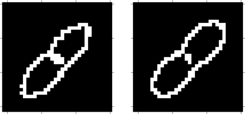
Figure 2: Left panel: original critical curve of a simulated cluster. Right panel: critical curve reconstructed with the algorithm proposed by Meneghetti et al. (2005); see the text for details. Only the central part of the cluster is shown. The corresponding side length is $\approx 1^{\prime}$ with pixel size of $\approx 2^{\prime\prime}$.

Figure 3 shows two-dimensional reconstructions of two projections of the simulated cluster after applying the strong-lensing correction in their cores. The coarse-grid resolution far from the cluster centre is increased near the core where the critical curve of the cluster is located. The resolution of the fine grid is 16 times higher (per dimension) than that of the coarse grid, so that pixels of the fine grid have $\sim 2^{\prime\prime}$ side length.

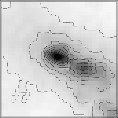
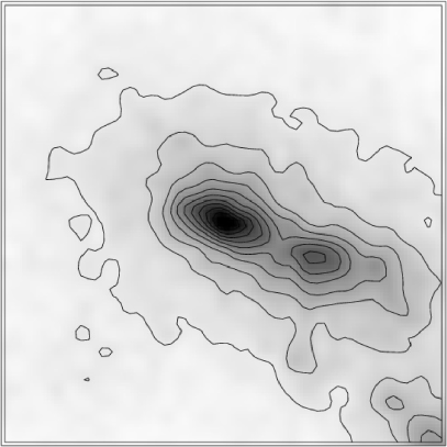
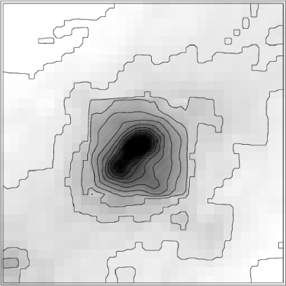
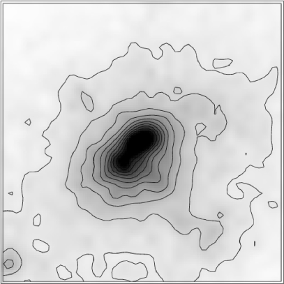
Figure 3: Two simulated clusters are shown in the two rows. Their original convergence fields are displayed in the right column, their joint reconstructions using weak and strong lensing in the left. The colour scale is linear, the grey scales range from $0$ to $1.1$, and the contours are spaced by $\Delta\kappa=0.1$.

The quality of the combined reconstruction is also illustrated in Fig. 4 by a map of the relative differences between our reconstruction and the original convergence of the simulated cluster. Evidently, the mass distribution is well reproduced everywhere in the field (see the caption for a quantitative description), in agreement with the good recovery of the radial profile. Moreover, constraints from strong lensing substantially improve the reconstruction in the cluster core. This demonstrates that the algorithm is working as expected.

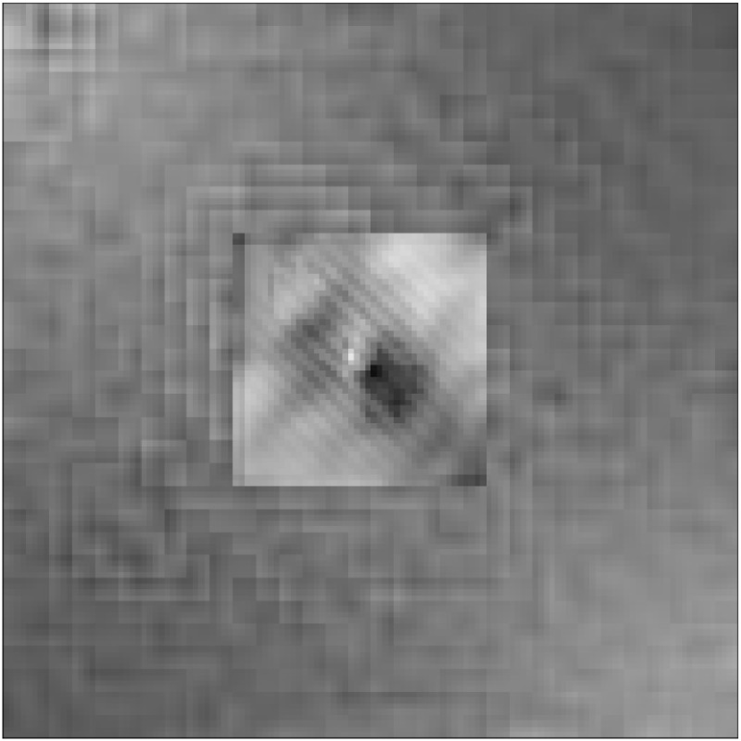
Figure 4: Deviation of the reconstructed from the original convergence fields, $\kappa$ and $\bar{\kappa}$, respectively. To avoid divergences near the field boundaries where both $\kappa$ and $\bar{\kappa}$ are small, the grey scale encodes the relative difference between $(1+\kappa)$ and $(1+\bar{\kappa})$, i.e. $(\kappa-\bar{\kappa})/(2+\kappa+\bar{\kappa})$. The grey scale ranges from $-0.1$ (white) to $+0.1$ (black). Obviously, the relative deviations are very small.

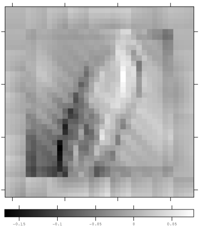
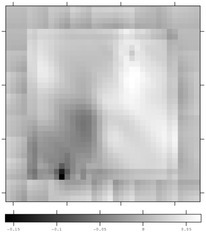
Figure 5: Both panels show the relative deviations between two reconstructed convergences $\kappa$ in the centre of a galaxy cluster. As in Fig. 4, the grey scale ranging from $-0.15$ (black) to $+0.1$ (white) encodes $(\kappa-\bar{\kappa})/(2+\kappa+\bar{\kappa})$ to avoid divergences for $|\kappa|\approx 0$. In both cases, the critical curve reconstructed with the method proposed by Meneghetti et al. (2005) is used instead of the precise critical curve. Left panel: Critical points are randomly shifted in the radial direction by one pixel or $\sim 2^{\prime\prime}$ prior to the reconstruction. While this procedure exaggerates realistic uncertainties, it provides an upper limit for the reconstruction errors which are $\lesssim 10\%$ almost everywhere in the field. Right panel: Only $16\%$ or 15 pixels of the critical curve are used, split into two sections opposing each other at the far ends of the critical curve. A random uncertainty in their positions is also included. Deviations are typically below $\sim 10\%$.

Figure 4 summarises the principal properties of our reconstruction method. The outer region (with low resolution) is well reproduced using only weak-lensing constraints, but the high-density peak near the cluster core is poorly resolved. The reconstruction of the core structure is greatly improved by adding the constraints from strong lensing. Given the quality of the results, we did not need to apply the iterative algorithm suggested above for correcting the relation between measured ellipticities and shear.

5.2.2 Approximate and partial knowledge of the critical curve

Since our joint reconstruction algorithm rests on the approximate knowledge of at least parts of the critical curve, we now investigate two main sources of uncertainty, namely position errors in the critical curve and incomplete knowledge of its location. For this purpose, we run reconstructions taking these aspects into account. Throughout, we do not assume precise knowledge of the simulated cluster’s critical curve, but reconstruct it using the method by (Meneghetti et al., 2005, see also Sand et al. 2004). Positional errors of $\lesssim 0.2^{\prime\prime}$ are found there. Since this is approximately the spatial resolution of the fine grid on which we reconstruct the convergence, we perform a reconstruction after randomly dislocating critical points by one pixel each. This procedure yields an upper limit to the effect of positional uncertainties in the critical curves.

The left panel of Fig. 5 displays the relative difference between the convergences reconstructed from the randomly shifted and the original critical curves. The figure suggests that the algorithm is working well because the inaccuracies in the critical curve cause relative deviations at a typical level of a few per cent.

Addressing the second source of uncertainty, we assume that only part of the critical curve is available (e.g. from the positions and orientations of one or more arcs). The right panel of Fig. 5 shows the relative differences between one reconstruction using the entire critical curve, and one using only $16\%$ or 15 pixels of it. Mimicking real observations, we further assume that this fraction of the critical curve is split into two approximately equal sections at the far ends of the critical curve. This approach simulates the presence of two arcs on opposite sides of a cluster. The relative differences are remarkably low, ranging around a few per cent and approaching $10\%$ only in few points.

The above tests confirm the underlying idea that a reconstruction based on joining weak and strong lensing features by using even part of the critical curve is feasible. The main sources of uncertainty do not substantially affect the method.

6 Conclusions

We have proposed a novel method for galaxy-cluster reconstruction which combines weak and strong-lensing data. The method is based on a least-$\chi^{2}$ fitting of the lensing potential $\psi$ (Bartelmann et al., 1996; Seitz et al., 1998) and exploits the fact that the $\chi^{2}$ minimisation can be carried out efficiently by inverting a sparse matrix (Bradač et al., 2005a, b). Contrary to other methods proposed for joining weak and strong lensing information (Bradač et al., 2005b; Diego et al., 2005), we propose to constrain the lensing potential obtained from the weak-lensing data by the approximate location of the critical curves, where the Jacobian determinant of the lens mapping must be close to zero.

The angular resolution which can be achieved by weak-lensing cluster reconstructions is typically of order $0.5^{\prime}$ for background source densities near $(30-40)\,\mathrm{arcmin^{-2}}$. This is much too coarse for tracing critical curves, whose typical sizes are $(0.5-1)^{\prime}$. Thus, we propose to cover those regions of the cluster fields with a refined grid where strong-lensing constraints are available.

We test the performance of the method on synthetic images produced with simulated lensing clusters. We conclude that the mass distribution in galaxy clusters is well reproduced across the entire field, in particular where constraints from strong lensing features are introduced. In practice, our algorithm first finds a lensing potential on the coarse grid which fits the weak-lensing data best. This approximation to the potential is then interpolated into the cells of the fine grid covering the critical curves or parts thereof, and refined by a $\chi^{2}$ minimisation taking the strong-lensing constraints into account.

We have used several approximations here. First, we treat weak lensing to first order in the shear $\gamma$, i.e. we compare measured ellipticities to $\gamma$ rather than the reduced shear $g=\gamma(1-\kappa)^{-1}$. Retaining the desirable linearity of the method, this can easily be overcome by introducing an iteration scheme in which the convergence $\kappa$ reconstructed in the previous step is used to update the reduced shear of the current step (see also Bradač et al. 2005b). Given the quality of our simulated results, we did not need to use this iteration scheme.

Second, we have assumed knowledge of the entire critical curve, which is of course not directly observable. Cluster images such as those recently taken with ACS on-board HST, however, show so many large arcs that critical curves can in fact be well constrained all around the cluster cores. Furthermore, critical curves can reliably be inferred from parametrised strong-lensing models, in particular when combined with dynamical constraints from central cluster galaxies (e.g. Meneghetti et al. 2005).

Third, we have assumed the strongly-lensed sources to be all at the same redshift. If multiple arc systems at different redshifts are observed, a lensing potential can still be reconstructed for one fiducial source redshift $\bar{z}_{\mathrm{s}}$ by applying the distance correction factors defined in (2).

Thus, we believe that the simplifications used here are not at all restrictive, and that the method suggested here provides a useful alternative to those proposed earlier. Our tests with randomly displaced critical points and partial knowledge of critical curves demonstrate that the method works well even in presence of positional uncertainties and gaps in the known critical curve.

Appendix A Linear equations for $\chi^{2}$ minimisation

We summarise here some technical aspects of how the physical quantities $\kappa$ and $\gamma$ are related to the discretised deflection potential $\psi$ in our approach.

Derivatives of $\psi$ are replaced by common finite-differencing schemes. We use 9 grid points for $\kappa$, 7 grid points for $\gamma_{2}$ and 4 points for $\gamma_{1}$. This allows any lensing quantity to be written as the multiplication of a well-defined matrix with the vector of lensing-potential values,

$$\kappa_{i}=\mathcal{K}_{ij}\psi_{j}\quad,\quad\gamma_{i}^{1}=\mathcal{G}_{ij}^{1}\psi_{j}\quad\hbox{and}\quad\gamma_{i}^{2}=\mathcal{G}_{ij}^{2}\psi_{j}\;.$$ (23)

The matrices $\mathcal{G}^{i}$ and $\mathcal{K}$ are very sparse because the finite-differencing schemes use only near neighbours (cf. Bradač et al. 2005b). Algorithms exist for efficient inversion of such matrices.

Based on the finite-differencing schemes expressed by the matrix Eqs.. (23), the minimisation of $\chi^{2}$ is reduced to a linear algebraic equation. Starting from the $\chi_{\mathrm{w}}^{2}$ for weak lensing, we have

$$0 = \frac{\partial{\chi_{w}}^{2}(\psi_{k})}{\partial\psi_{j}}$$ (24)

$$= -2\sum_{i=1}^{n}\frac{1}{\sigma_{wi}^{2}}\left[(\epsilon_{i}^{1}-\gamma_{i}^{1})\frac{\partial\gamma_{i}^{1}}{\partial\psi_{j}}+(\epsilon_{i}^{2}-\gamma_{i}^{2})\frac{\partial\gamma_{i}^{2}}{\partial\psi_{j}}\right]$$

$$= \sum_{i=1}^{n}\frac{-2}{\sigma_{wi}^{2}}\left[(\epsilon_{i}^{1}-\gamma_{i}^{1})\frac{\partial\left(\mathcal{G}^{1}_{ik}\psi_{k}\right)}{\partial\psi_{j}}+(\epsilon_{i}^{2}-\gamma_{i}^{2})\frac{\partial\left(\mathcal{G}^{2}_{ik}\psi_{k}\right)}{\partial\psi_{j}}\right]$$

$$= \sum_{i=1}^{n}\frac{-2}{\sigma_{wi}^{2}}\left[(\epsilon_{i}^{1}-\gamma_{i}^{1})\mathcal{G}^{1}_{ik}\delta_{jk}+(\epsilon_{i}^{2}-\gamma_{i}^{2})\mathcal{G}^{2}_{ik}\delta_{jk}\right]$$

$$= \sum_{i=1}^{n}\frac{-2}{\sigma_{wi}^{2}}\left[(\epsilon_{i}^{1}-\gamma_{i}^{1})\mathcal{G}^{1}_{ij}+(\epsilon_{i}^{2}-\gamma_{i}^{2})\mathcal{G}^{2}_{ij}\right]$$

$$= \sum_{i=1}^{n}\frac{-2}{\sigma_{wi}^{2}}\Big{[}\epsilon_{i}^{1}\mathcal{G}^{1}_{ij}-\mathcal{G}^{1}_{ij}\mathcal{G}^{1}_{ik}\psi_{k}+\epsilon_{i}^{2}\mathcal{G}^{2}_{ij}-\mathcal{G}^{2}_{ij}\mathcal{G}^{2}_{ik}\psi_{k}\Big{]}$$

$$= \sum_{i=1}^{n}\frac{2}{\sigma_{wi}^{2}}\left\{\left[\mathcal{G}^{1T}_{ji}\mathcal{G}^{1}_{ik}+\mathcal{G}^{2T}_{ji}\mathcal{G}^{2}_{ik}\right]\psi_{k}-\left[\epsilon_{i}^{1}\mathcal{G}^{1}_{ij}+\epsilon_{i}^{2}\mathcal{G}^{2}_{ij}\right]\right\}\;,$$

which can clearly be written in the form

$$\mathcal{B}_{jk}\psi_{k}=\mathcal{V}_{j}\;,$$ (25)

with the matrix

$$\mathcal{B}_{jk}\equiv\sum_{i=1}^{n}\frac{1}{\sigma_{wi}^{2}}\left[\mathcal{G}_{ji}^{1T}\mathcal{G}_{ik}^{1}+\mathcal{G}_{ji}^{2T}\mathcal{G}_{ik}^{2}\right]$$ (26)

and the data vector

$$\mathcal{V}_{j}=\sum_{i=1}^{n}\frac{1}{\sigma_{wi}^{2}}\Big{[}\epsilon^{1}_{i}\mathcal{G}_{ij}^{1}+\epsilon^{2}_{i}\mathcal{G}_{ij}^{2}\Big{]}\;.$$ (27)

Similarly evaluating the constraints from strong lensing yields

$$\frac{\partial\chi_{\mathrm{s}}^{2}}{\partial\psi^{*}_{j^{\prime}}} = \frac{\partial}{\partial\psi^{*}_{j^{\prime}}}\left[\sum_{i=1}^{n*}\frac{(\det\mathcal{A}_{i})^{2}}{\sigma^{2}_{i}}\right]$$ (28)

$$= \sum_{i=1}^{n*}\frac{-4\det\mathcal{A}_{i}}{\sigma^{2}_{i}}\left[(1-\kappa_{i})\frac{\partial\kappa_{i}}{\partial\psi^{*}_{j^{\prime}}}-\frac{\partial\gamma_{i}^{1}}{\partial\psi^{*}_{j^{\prime}}}-\frac{\partial\gamma_{i}^{2}}{\partial\psi^{*}_{j^{\prime}}}\right]$$

$$= \sum_{i=1}^{n*}\frac{-4\det\mathcal{A}_{i}}{\sigma^{2}_{i}}\left[(1-\kappa_{i})\mathcal{K}_{ij^{\prime}}-\gamma_{i}^{1}\mathcal{G}^{1}_{ij^{\prime}}-\gamma_{i}^{2}\mathcal{G}^{2}_{ij^{\prime}}\right]$$

$$= \mathcal{T}_{j^{\prime}}\;,$$

where the $\kappa_{i}$ and the $\gamma_{i}^{1,2}$ are obtained from the interpolated weak-lensing solution.

On the refined grid, the $\chi^{2}$ minimisation (25) is modified by

$$\mathcal{B}_{jk}\psi_{k}^{*}=\mathcal{V}_{j}-\mathcal{T}_{j^{\prime}}\;.$$ (29)

Obviously, if the weak-lensing solution already satisfies $\det\mathcal{A}=0$ on the critical curves, $\mathcal{T}=0$ there, and no correction is necessary.

References

- Bartelmann et al. (1998) Bartelmann, M., Huss, A., Colberg, J. M., Jenkins, A., & Pearce, F. R. 1998, A&A, 330, 1
- Bartelmann et al. (1996) Bartelmann, M., Narayan, R., Seitz, S., & Schneider, P. 1996, ApJL, 464, L115
- Bradač et al. (2005a) Bradač, M., Erben, T., Schneider, P., et al. 2005a, A&A, 437, 49
- Bradač et al. (2005b) Bradač, M., Schneider, P., Lombardi, M., & Erben, T. 2005b, A&A, 437, 39
- Brainerd et al. (1996) Brainerd, T. G., Blandford, R. D., & Smail, I. 1996, ApJ, 466, 623
- Broadhurst et al. (2005) Broadhurst, T., Benítez, N., Coe, D., et al. 2005, ApJ, 621, 53
- Diego et al. (2005) Diego, J. M., Tegmark, M., Protopapas, P., & Sandvik, H. B. 2005, ArXiv Astrophysics e-prints, arXiv:astro-ph/0509103
- Falco et al. (1985) Falco, E. E., Gorenstein, M. V., & Shapiro, I. I. 1985, ApJ, 289, L1
- Ford et al. (1996) Ford, H. C., Feldman, P. D., Golimowski, D. A., et al. 1996, in Proc. SPIE Vol. 2807, p. 184-196, Space Telescopes and Instruments IV, Pierre Y. Bely; James B. Breckinridge; Eds., ed. P. Y. Bely & J. B. Breckinridge, 184–196
- Grossman & Narayan (1988) Grossman, S. A. & Narayan, R. 1988, ApJL, 324, L37
- Grossman & Narayan (1989) Grossman, S. A. & Narayan, R. 1989, ApJ, 344, 637
- Kovner (1989) Kovner, I. 1989, ApJ, 337, 621
- Meneghetti et al. (2005) Meneghetti, M., Bartelmann, M., Jenkins, A., & Frenk, C. 2005, ArXiv Astrophysics e-prints; arXiv:astro-ph/0509323
- Rix et al. (2004) Rix, H.-W., Barden, M., Beckwith, S. V. W., et al. 2004, ApJS, 152, 163
- Sand et al. (2004) Sand, D. J., Treu, T., Smith, G. P., & Ellis, R. S. 2004, ApJ, 604, 88
- Schneider et al. (1992) Schneider, P., Ehlers, J., & Falco, E. E. 1992, Gravitational Lenses (Springer Verlag, Heidelberg)
- Schneider & Seitz (1995) Schneider, P. & Seitz, C. 1995, A&A, 294, 411
- Seitz et al. (1998) Seitz, S., Schneider, P., & Bartelmann, M. 1998, A&A, 337, 325