Big Bang nucleosynthesis in scalar tensor gravity: the key problem of the primordial ⁷Li abundance

Abstract

Combined with other CMB experiments, the WMAP survey provides an accurate estimate of the baryon density of the Universe. In the framework of the standard Big Bang Nucleosynthesis (BBN), such a baryon density leads to predictions for the primordial abundances of ⁴He and D in good agreement with observations. However, it also leads to a significant discrepancy between the predicted and observed primordial abundance of ⁷Li. Such a discrepancy is often termed as ’the lithium problem’. In this paper, we analyze this problem in the framework of scalar-tensor theories of gravity. It is shown that an expansion of the Universe slightly slower than in General Relativity before BBN, but faster during BBN, solves the lithium problem and leads to ⁴He and D primordial abundances consistent with the observational constraints. This kind of behavior is obtained in numerous scalar-tensor models, both with and without a self-interaction potential for the scalar field. In models with a self-interacting scalar field, the convergence towards General Relativity is ensured without any condition, thanks to an attraction mechanism which starts to work during the radiation-dominated epoch.

1 Introduction

The Big Bang Nucleosynthesis prediction for the ⁴He primordial abundance is traditionally considered as a good estimate of the baryon density of the Universe. However, the recent measurement of the Cosmic Microwave Background (CMB) anisotropies by WMAP (Bennett & al, 2003) now provides, when combined with other CMB experiments (CBI and ACBAR), another accurate estimate of the baryon density: $\Omega_{b}h^{2}=0.0224\pm 0.0009$ (or $\eta\times 10^{10}=6.14\pm 0.25$ in terms of the baryon to photon ratio) (Spergel & al, 2003). This value of $\eta$ can be used to compute the primordial abundances of light elements (mainly ⁴He, ³He, D and ⁷Li). The comparison of predicted and observed abundances is then a way to test the concordance between BBN and the CMB data.

When one assumes the WMAP estimate of the baryon to photon ratio, the primordial abundances predicted by the standard BBN ( i.e. three families of light neutrinos, a neutron mean life $\tau_{n}=885.7\pm 0.8s$, gravitation described by General Relativity and a homogeneous and isotropic Universe) are (Cyburt & al, 2003):

$$\mbox{Y}_{p} = 0.2484^{+0.0004}_{-0.0005}$$

D/H $$= 2.75^{+0.24}_{-0.19}\times 10^{-5}$$

$${}^{7}\mbox{Li/H} = 3.82^{+0.73}_{-0.60}\times 10^{-10}$$

while the observed abundances are:

$$\mbox{Y}_{p} = \left\{\begin{array}[]{ll}0.2391\pm 0.0020&\mbox{ ref. \cite[citep]{(\@@bibref{AuthorsPhrase1Year}{Luridiana2003}{\@@citephrase{, }}{})}}\\ 0.2452\pm 0.0015&\mbox{ ref. \cite[citep]{(\@@bibref{AuthorsPhrase1Year}{Izotov1999}{\@@citephrase{, }}{})}}\end{array}\right.$$ (3)

D/H $$= 2.78^{+0.44}_{-0.38}\times 10^{-5}\mbox{ ref. \cite[citep]{(\@@bibref{AuthorsPhrase1Year}{Kirkman2003}{\@@citephrase{, }}{})}}$$ (4)

$${}^{7}\mbox{Li/H} = \left\{\begin{array}[]{ll}1.23^{+0.68}_{-0.32}\times 10^{-10}&\mbox{ ref. \cite[citep]{(\@@bibref{AuthorsPhrase1Year}{Ryan2000}{\@@citephrase{, }}{})}}\\ 2.19^{+0.46}_{-0.38}\times 10^{-10}&\mbox{ ref. \cite[citep]{(\@@bibref{AuthorsPhrase1Year}{Bonifacio2002}{\@@citephrase{, }}{})}.}\end{array}\right.$$ (7)

Here, the two values for the observed $Y_{p}$ correspond to independent estimates in refs. (Luridiana & al, 2003) and (Izotov & al, 1999) based on observations of metal-poor extragalactic ionized hydrogen regions. The D abundance is determined by observations of remote cosmological clouds on the line of sight of high redshift quasars. Finally the ⁷Li/H estimate of Ryan & al (2000) has been performed by observing halo stars, while the value of Bonifacio & al (2002) comes from the observation of stars in the globular cluster NGC 6397. Although some recent estimates (Boesgaard & al, 2005) leads to a somewhat smaller value, several other independent determinations (Ryan & al, 1999; Thevenin & al, 2001; Asplung & al, 2005) obtain observed primordial abundances of ⁷Li/H similar to those reported either by Ryan & al (2000) or Bonifacio & al (2002).

We can see a relatively good agreement for the predicted and observed abundances of ⁴He and D, but a large discrepancy for ⁷Li/H. There had been many attempts to account for the low ⁷Li abundance indicated by observations. The first and most conservative possibility is the existence of systematic uncertainties in the observational determination of the ⁷Li abundance. However, such uncertainties are not large enough to solve the problem (see Ryan & al (2000) and Bonifacio & al (2002)). In the same way, the systematic study of uncertainties on the nuclear reaction rates performed in Coc & al (2004) indicates that these uncertainties cannot explain the large discrepancy emphasized before. Modifications of the standard nucleosynthesis scenario then arise as possible ways to reconcile the predictions with the observations. Inhomogeneous nucleosynthesis has been analyzed (Jedamzik & Rehm, 2001) but overproduces ⁷Li. Late particles decays can deplete ⁷Li, but they cannot account for the observed D and D/³He primordial abundances (Jedamzik1, 2004; Jedamzik2, 2004; Ellis & al, 2005); another possibility is provided by the creation of baryons after BBN, accompanied by a lepton asymmetry before BBN, the two processes arising from Q-balls (Ichikawa & al, 2004).

In this work, we will address the lithium abundance problem in the framework of scalar-tensor theories of gravity (Brans & Dicke, 1961; Bergmann, 1968; Wagoner, 1970; Nordvedt, 1970). In these theories, gravitation is modified by the introduction of a scalar degree of freedom, which does not affect the standard nuclear and particle physics. Such modifications arise as low-energy limits of superstrings theories (Green & al, 1988) and they provide a way to change the expansion history of the Universe with minimal assumptions. We will show that such theories contain a mechanism that could be responsible for a low lithium abundance, despite the high baryon to photon ratio implied by the WMAP estimate. Big Bang Nucleosynthesis in the context of a scalar-tensor cosmology has been extensively studied in the past (Wagoner, 1973; Barrow, 1978; Serna & Alimi, 1996; Alimi & Sena, 1997; Serna & al, 2002; Clifton & al, 2005; Coc & al, 2006), but the main goal of these works was to constrain the parameters of the theory thanks to the primordial abundances of ⁴He, D and ⁷Li, or to obtain the observed abundances with a matter density of the Universe different from its commonly assumed value. Moreover, general self-interacting scalar fields were not considered and, as we will see later, the introduction of such terms in the lagrangian can provide the mechanism necessary to explain the low ⁷Li abundance.

The paper is arranged as follows. In Section 2, the scalar-tensor gravity theories and the implied cosmological models are presented. Then, in Section 3, we analyze the lithium problem in the framework of different kinds of scalar tensor theories. We show that the solution of this problem requires a non trivial dynamics for the scalar field at the epoch of BBN. Finally, we discuss the generality of that solution.

2 Scalar-tensor cosmological model

2.1 Equations and observable quantities

In scalar-tensor theories of gravity, the dynamics of the Universe contains a new scalar degree of freedom that couples explicitly to the energy content of the Universe. In units of $c=1$, the action generically writes, in the Einstein frame:

$$S = \frac{1}{4\pi G_{*}}\int\left(\frac{R^{*}}{4}-\frac{1}{2}\varphi_{,\mu}\varphi^{\mu}-V(\varphi)\right)\sqrt{-g^{*}}d^{4}x$$ (8)

$$+ S_{m}(\psi_{m},A^{2}(\varphi)g_{\mu\nu}^{*}),$$

$G_{*}$ being a bare gravitational constant, $\varphi$ the scalar field, $V(\varphi)$ its self-interaction term and $A(\varphi)$ its coupling to matter. The functional $S_{m}(\psi_{m},A^{2}(\varphi)g_{\mu\nu}^{*})$ stands for the action of any field $\psi_{m}$ that contributes to the energy content of the Universe. It expresses the fact that all these fields couple universally to a conformal metric $g_{\mu\nu}=A^{2}(\varphi)g_{\mu\nu}^{*}$, then implying that the weak equivalence principle (local universality of free fall for non-gravitationally bound objects) holds in this class of theories. The metric $g_{\mu\nu}$ defines the Dicke-Jordan frame, in which standard rods and clocks can be used to make measurements (since in this frame, the matter part of the action acquires its standard form). Defining

$$\alpha(\varphi)=\frac{d\ln A(\varphi)}{d\varphi},$$ (9)

and considering the transformations:

$$g_{\mu\nu} = A^{2}(\varphi)g_{\mu\nu}^{*}$$

$$\phi = A^{-2}(\varphi)$$

$$U(\phi) = 2A^{4}(\varphi)V(\varphi)$$

$$|3+2\omega(\phi)| = \alpha^{-2}(\varphi)$$

the action in the Dicke-Jordan frame writes:

$$S = \frac{1}{16\pi G_{*}}\int\left(\phi R-\frac{\omega(\phi)}{\phi}\phi_{,\mu}\phi^{\mu}-U(\phi)\right)\sqrt{-g}d^{4}x$$ (10)

$$+ S_{m}(\psi_{m},g_{\mu\nu})$$

Despite the conformal relation, these two frames have a different status: in the Dicke-Jordan frame, where the gravitational degrees of freedom are mixed, the lagrangian for the matter fields does not contain explicitly the new scalar field: the non gravitational physics has then its standard form. In the Einstein frame, the scalar degree of freedom explicitly couples to the matter fields, then leading for example to the variation of the inertial masses of point-like particles. Of course, the two frames describe the same physical world. Nevertheless, the usual interpretation of the observable quantities is profoundly modified in the Einstein frame, whereas it holds in the Dicke-Jordan frame, where the rods and clocks made with matter are not affected by the presence of the scalar field. That is why we will refer to the Dicke-Jordan frame as the observable one.

Varying the Einstein frame action (8) with respect to the fields yields the equations:

$$R^{*}_{\mu\nu}-\frac{1}{2}R^{*}g^{*}_{\mu\nu} = 8\pi G_{*}T^{*}_{\mu\nu}+T^{\varphi}_{\mu\nu}$$ (11)

$$\Box^{*}\varphi = -4\pi G_{*}\alpha(\varphi)T_{*}+\frac{dV(\varphi)}{d\varphi}$$ (12)

$$\nabla^{*}_{\nu}T^{\nu}_{*\mu} = \alpha(\varphi)T_{*}\nabla^{*}_{\mu}\varphi$$ (13)

where $T_{*}$ is the trace of the energy-momentum tensor of matter fields $T_{*\mu\nu}$, related to the observable one by $T_{\mu\nu}=A^{-2}(\varphi)T_{*\mu\nu}$, and $T^{\varphi}_{\mu\nu}=2\varphi_{,\mu}\varphi_{,\nu}-g^{*}_{\mu\nu}(g_{*}^{\alpha\beta}\varphi_{\alpha}\varphi_{\beta})-2V(\varphi)g^{*}_{\mu\nu}$ is the energy-momentum tensor of the scalar field. It is important to note that these equations reduces to those of General Relativity in presence of a scalar field if $\alpha(\varphi)=0$.

Except when the contrary is explicitly stated, all the computations presented in this paper have been performed in the Einstein frame, because it leads to well posed Cauchy problems (that is elliptic and/or hyperbolic equations with a set of initial conditions) and has a perfectly regular dynamics. Nevertheless, the cosmological evolution resulting from these computations was later expressed in the Dicke-Jordan frame, where the interpretation of the observable quantities is easier.

2.2 Homogeneous and isotropic Universe

Under the assumption of a Universe filled with various homogeneous and isotropic matter fluids, the metric reduces to the Friedman-Lemaître-Robertson-Walker (FLRW) form in the observable Dicke-Jordan frame:

$$ds^{2} = -dt^{2}+a^{2}(t)dl^{2}$$

$$dl^{2} = \frac{dr^{2}}{1-kr^{2}}+r^{2}(d\theta^{2}+sin^{2}\theta d\psi^{2})$$

and, also in the Einstein frame because of the conformal relation:

$$ds_{*}^{2} = -dt_{*}^{2}+a_{*}^{2}(t*)dl^{2}$$

with $dt=A(\varphi(t_{*}))dt_{*}$ and $a(t)=A(\varphi(t_{*}))a_{*}(t_{*})$.

Then, defining $H_{*}=(1/a_{*})(da_{*}/dt_{*})$, the fields equations (11) become:

$$H_{*}^{2}=\frac{8\pi G_{*}\rho_{*}}{3}+\frac{1}{3}\dot{\varphi}^{2}+\frac{2}{3}V(\varphi)-\frac{k}{a_{*}^{2}(t_{*})}$$ (14)

$$-3\frac{\ddot{a_{*}}}{a_{*}}=4\pi G_{*}(\rho_{*}+3p_{*})+2\dot{\varphi}^{2}-2V(\varphi)$$ (15)

$$\ddot{\varphi}+3H_{*}\dot{\varphi}+\frac{dV(\varphi)}{d\varphi}=-4\pi G_{*}\alpha(\varphi)(\rho_{*}-3p_{*})$$ (16)

where dots denote derivatives with respect to $t_{*}$, whereas $\rho_{*}$ and $p_{*}$ are the total mass-energy density and pressure, respectively. They are conformally related to the energy density $\rho$ and the pressure $p$ in the Jordan frame by $\rho_{*}=A^{4}(\varphi)\rho$ and $p_{*}=A^{4}(\varphi)p$. The observable Hubble parameter $H(t)$ is related to the Einstein frame quantities by

$$H(t)=\frac{1}{A(\varphi)}(H_{*}(t_{*})+\alpha(\varphi(t_{*}))\dot{\varphi}(t_{*}))$$ (17)

2.3 Dynamics of the scalar field

In the form given above, the time evolution of the scalar field is coupled, both in the Dicke-Jordan and the Einstein frame, to that of the scale factor. Previous works (Serna & al, 2002; Damour & Nordvedt, 1993) have found that, by introducing an appropriate change of variables, it is possible to obtain an evolution equation for the scalar field which is independent of the cosmic scale factor. Such an equation allows for the dynamical analysis of any scalar tensor theory and, in particular, its asymptotic behavior at early and late times. When the latter behavior implies a convergence mechanism towards General Relativity, one can ensures that the Solar System constraints will be satisfied. We will now extend such previous works to the general case of scalar-tensor theories with a self-interaction term.

Introducing a new evolution parameter $\lambda=\ln a_{*}+const$, so that $d\lambda=H_{*}dt_{*}$, and denoting $u^{\prime}=du/d\lambda$, the evolution equations (14)-(16) lead to:

$$\frac{2(1-\epsilon+\eta)}{3-\varphi^{\prime 2}}\varphi^{\prime\prime} +(1-w_{b}-\frac{4}{3}\epsilon+2\eta)\varphi^{\prime}$$

$$= -\Theta-(1-3w_{b})\alpha(\varphi)$$ (18)

where

$$\epsilon(\lambda) = \frac{3k}{8\pi G_{*}\rho_{*}(\lambda)a_{*}^{2}(\lambda)}$$

$$\eta(\varphi,\lambda) = \frac{V(\varphi)}{4\pi G_{*}\rho_{*}(\lambda)}$$

$$w_{b} = \frac{p_{*}}{\rho_{*}}$$

$$\Theta(\varphi,\lambda) = \frac{\frac{dV(\varphi)}{d\varphi}}{4\pi G_{*}\rho_{*}(\lambda)}$$

This equation is similar, but not equivalent, to the motion equation of a mechanical oscillator with a varying ”mass” $m_{eff}=2(1-\epsilon+\eta)/(3-\varphi^{\prime 2})$, a varying ”friction” $\nu_{eff}=(1-w_{b}-4\epsilon/3+2\eta)$ and a ”force” term $F_{eff}=-\Theta-(1-3w_{b})\alpha$. Then, one can define an effective potential $V_{eff}(\varphi,\lambda)$ that verifies the relation:

$$\frac{\partial V_{eff}(\varphi,\lambda)}{\partial\varphi} = \Theta(\varphi,\lambda)+(1-3w_{b})\alpha(\varphi)$$ (19)

In the following, we will only consider flat cosmologies ($\epsilon=0$). In these cases, the ”friction” term $(1-w_{b}+2\eta)$ is always positive, and the dynamics of the scalar field is then analogous to a damped oscillating motion in the effective potential $V_{eff}(\varphi,\lambda)$. Such an effective potential (see Eq. (19)) presents two different parts: a term due to the coupling function $\alpha(\varphi)$ and another term due to the self-interaction $V(\varphi)$ of the scalar field.

During the matter-dominated era ($w_{b}=0$), both terms are important to determine the effective potential. The minima of $V_{eff}$ will be attractors for the dynamics of the scalar field and determine the behavior of the theory at late times. Consequently, if the relativistic value $\varphi=0$ is a minimum of this effective potential, the theory will converge towards General Relativity.

Instead, during the radiation-dominated era ($w_{b}=1/3$), the only non-vanishing contribution to the effective potential is that due the self-interaction of the scalar field. Equation (2.3) then reduces to:

$$\frac{2(1+\eta)}{3-\varphi^{\prime 2}}\varphi^{\prime\prime}+\frac{2}{3}(1+3\eta)\varphi^{\prime}=-\Theta$$ (20)

At very early times, when $\rho_{*}$ is very high, $\Theta\sim\eta\sim 0$ so that self-interaction has a negligible effect on the scalar field dynamics. In this case ($\Theta\sim\eta\sim 0$), the integration of equation (20) gives:

$$\varphi^{\prime 2}=\frac{3k^{2}}{e^{2\lambda}+k^{2}}$$ (21)

where $k$ is a constant related to the value of $\varphi^{\prime}$ at $\lambda=0$ through $k^{2}=\varphi^{\prime 2}_{0}/(3-\varphi^{\prime 2}_{0})$. Note that the above equation implies that $-\sqrt{3}<\varphi^{\prime}<\sqrt{3}$.

One can see from equation (21) that the velocity of the scalar field exponentially decreases with $\lambda$ at very early times. When the initial ($\lambda=0$) velocity is not very high (i.e., when it is not close to $\sqrt{3}$), one can assume that the scalar field reaches the epochs of interest (those prior to BBN processes) with an almost vanishing velocity:

$$\varphi^{\prime}=0\mbox{$\;\;$(before BBN)}.$$ (22)

For the sake of simplicity, we will consider throughout this paper a vanishing initial value of the scalar field velocity (see the Appendix for some examples where such a condition has been relaxed). Hereafter, all quantities at this initial time (prior to BBN) will be expressed with a subscript ’init’.

The condition (22) does not however imply a constant $\varphi$ value during the whole radiation-dominated epoch. Since $\rho_{*}$ is a decreasing function of $\lambda$, the contribution of $V(\varphi)$ to the effective potential will become non-negligible at some ’time’ $\lambda$. If $V(\varphi)$ is chosen to be a function having a minimum at $\varphi_{m}$, the scalar field will start to be attracted towards $\varphi_{m}$. For example, the simple choice of a power law $V(\varphi)\propto\varphi^{2n}$ for the self-interaction term, will imply an attraction mechanism towards General Relativity which starts to work during the radiation-dominated epoch.

3 BBN in scalar-tensor theories

We will now analyze the BBN processes, and the resulting primordial abundances, in the framework of scalar-tensor theories both with and without a self-interaction term. As stated above, we will consider throughout this section that the initial value of the scalar field is a free parameter, while its initial velocity is fixed to $\dot{\varphi}_{init}=0$. The initial values of the remaining variables are chosen so that they imply a flat Universe and lead, at the present temperature $T_{0}=2.725$, to cosmological parameters given by: $\Omega_{m,0}=0.27$, $\Omega_{\Lambda,0}=0.73$ and $H_{0}=71\mbox{ km}\mbox{ s}^{-1}\mbox{Mpc}^{-1}$. We assume an standard particle content of the Universe, with three families of light neutrinos, and the WMAP estimate of the present baryon to photon ratio ($\eta\times 10^{10}=6.14\pm 0.25$).

The numerical computation consists of two main parts: first, we use a sixth-order Runge-Kutta integrator to fully determine the cosmological model and, in particular, the evolution of the expansion rate. Once determined the cosmological evolution in a given gravitational theory, we compute the BBN processes and the resulting primordial abundances of light elements thanks to a complex network of 28 nuclear reactions, and using the Beaudet and Yahil scheme (Beaudet & Yahil, 1977). We used the reaction rates of Caughlan & Fowler (1998) and Smith & al (1993) and the updated reaction rates of the NACRE collaboration (Angulo & al, 1999). The only aspect that differs from the standard BBN in General Relativity is the expansion rate of the Universe. It impacts on the various nuclear abundances because they are determined by many reactions whose efficiency depends on the ratio of the reaction rates $\Gamma_{i}$ and the expansion rate $H$. Indeed, a reaction with rate $\Gamma_{i}$ is in equilibrium when $\Gamma_{i}/H>1$, whereas the reaction is frozen when $\Gamma_{i}/H<1$ . This is directly linked with the fact that the expansion dilutes the particles. Then, a modification in the expansion history may significantly change the nuclear abundances by modifying the dynamical structure of the network of reactions, making some reactions more efficient, and limiting others (it should be noted that this remark is valid for the nuclear reaction rates, and also for the rates of the weak interaction processes that take place before BBN and that interconvert neutrons and protons).

In order to characterize the deviation from General Relativity, it is convenient to introduce the speed-up factor, defined as the ratio between the expansion rate $H(T)$ and the corresponding expansion rate in General Relativity $H_{GR}(T)$ at the same temperature:

$$\xi(T)=\frac{H(T)}{H_{GR}(T)}$$ (23)

When $\xi(T)>1$ ($\xi(T)<1$ ), the Universe expands faster (slower) than in General Relativity at the temperature $T$.

3.1 Theories without a self-interaction term

We will first consider the simplest case of scalar-tensor models without a self-interaction term. In this case, the effective potential during the radiation-dominated epoch is (see equation (19)):

$$V_{eff}(\varphi)=0$$ (24)

and, since we are assuming the initial condition (22), the scalar field will be frozen to its initial value $\varphi_{init}$ (except for a slight temporary perturbation during the annihilation of electrons and positrons around $T=0.1\mbox{ MeV}$, when $w_{b}$ slightly deviates from $1/3$). Consequently, $\dot{\varphi}=0$ during all the BBN processes, and the relation (17) reduces to $H=H_{*}/A(\varphi_{i})$. Introducing the expression (14) for $H_{*}$ in this equation, we can write:

$$H(T) = \sqrt{\frac{8\pi G_{*}A^{2}(\varphi_{i})}{3}\rho}$$

$$= A(\varphi_{i})H_{GR}(T)$$

which implies $\xi\sim A(\varphi_{i})=$ constant.

Equation (3.1) shows that the dynamics of the Universe is the same as in General Relativity, but with an effective gravitational constant given by $G_{eff}=G_{*}A^{2}$, where $G_{*}=G_{N}$ is the usual Newtonian value ($G_{N}=6.673\times 10^{-11}\mbox{m}^{3}\mbox{ kg}^{-1}\mbox{ s}^{-2}$ ). Cyburt (Cyburt, 2004) has determined the scaling of the various primordial abundances in terms of the physical constants. In particular, when the dynamics of the Universe is governed by General Relativity, the scaling with the effective gravitational constant is:

$$\mbox{Y}_{p} = 0.2484\left(\frac{G_{eff}}{G_{N}}\right)^{0.35}$$ (26)

D/H $$= 2.75\left(\frac{G_{eff}}{G_{N}}\right)^{0.95}10^{-5}$$ (27)

$${}^{3}\mbox{He/H} = 8.65\left(\frac{G_{eff}}{G_{N}}\right)^{0.34}10^{-6}$$ (28)

$${}^{7}\mbox{Li/H} = 3.82\left(\frac{G_{eff}}{G_{N}}\right)^{-0.72}10^{-10}$$ (29)

Figure 1 shows these abundances as functions of $G_{eff}/G_{N}$, as well as their observational constraints. One clearly notes from this figure that there is no consistent value for $G_{eff}/G_{N}$ that can simultaneously account for all the observed abundances: the observed ⁷Li primordial abundance requires $G_{eff}/G_{N}>1.8$ while ⁴He and D impose $G_{eff}/G_{N}\sim 1$.

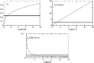
Figure 1: Primordial abundances as functions of $G_{eff}/G_{N}$. The shaded regions are the assumed observed abundances.

Consequently, in absence of a self-interaction term, scalar-tensor theories with an arbitrary coupling function $\alpha(\varphi)$ (with $\dot{\varphi}_{init}=0$) cannot constitute a solution for the lithium problem. The same conclusion can be found using the formulation of Kneller and Steigman (Kneller & Steigman, 2004)

3.2 Theories with a self-interaction term

We will now consider scalar-tensor models with a self-interaction term. As emphasized above, such a term acts as an effective potential even during the radiation-dominated epoch. Therefore, except for very early times (with a very high density), the scalar field does not remain frozen to its initial value and the speed-up factor is not necessarily a constant during the BBN processes.

Of course, depending on the functional form of $\alpha(\varphi)$ and $V(\varphi)$, there exist many theories that exhibit a varying speed-up factor. Before analyzing a particular choice for $\alpha(\varphi)$ and $V(\varphi)$, we may ask whether we can constrain the behavior of the speed-up factor in order to solve the ⁷Li problem without affecting the other abundances.

3.2.1 Computation of the primordial abundances

Since essentially all the neutrons are incorporated into ⁴He nuclei, the final production of ⁴He is directly related to the abundance of neutrons in epochs prior to the BBN processes. Indeed, $Y_{p}$ is roughly given by

$$Y_{p}\simeq\frac{2(n/p)_{fr}}{1+(n/p)_{fr}}$$ (30)

where $(n/p)_{fr}$ denotes the neutron to proton ratio when their weak reactions, $n+\nu_{e}\leftrightarrow p+e^{-}$ and $n+e^{+}\leftrightarrow p+\bar{\nu}_{e}$, freeze out of equilibrium. Such a ratio is then fixed at a temperature $T_{fr}$ of about 1 MeV, well before the synthesis of light elements (from $\sim 100$ KeV to $\sim 10$ KeV). The $(n/p)_{fr}$ ratio, and hence the final $Y_{p}$ value, strongly depends on $T_{fr}$ through:

$$(n/p)_{fr}=\exp(-Q/T_{fr})$$ (31)

where $Q$ is the difference between the neutron and proton masses. A faster (slower) expansion rate of the Universe implies a higher (lower) freezing-out temperature, resulting in higher (lower) neutron and ⁴He abundances.

The ⁷Li production is instead determined by the processes of BBN. In particular, when the baryon to photon ratio is greater than $3\times 10^{-10}$, the lithium is mainly produced through the reaction ${}^{3}\mbox{He}(\alpha,\gamma)^{7}\mbox{Be}$ followed by a decay of ⁷Be through electron captures (when $\eta<3\times 10^{-10}$, the lithium is instead produced by ${}^{3}\mbox{He}(\alpha,\gamma))^{7}\mbox{Li}$). Therefore, the final abundance of lithium strongly depends on both the helium production and the efficiency of the ⁴He burning to give ⁷Li. If $\Gamma_{i}$ denotes the reaction rate, such an efficiency is given by $\Gamma_{i}/H=(\Gamma_{i}/H_{RG})/\xi(T)$, so that a faster (slower) expansion rate of the Universe during BBN implies a less (more) efficient production of ⁷Li.

Since General Relativity leads to a predicted $Y_{p}$ value in agreement with observations, one can expect that any other gravity theory must imply a speed-up factor close to unity at $T\sim 1$ MeV, or slightly smaller than unity to favor a less efficient production of ⁷Li without implying an over-production of ⁴He. Later, during the BBN processes, a speed-up factor that has significantly increased above unity could help to solve the lithium problem. Obviously, since any gravity theory must converge at late times towards General Relativity (in order to be compatible with Solar System experiments), the increase of the speed-up factor must stop at some time and, afterwards, it must approach unity. Therefore, models implying a constant or monotonic $\xi(T)$ function are not good candidates to solve the lithium problem. We will then restrict our analysis to self-interacting scalar-tensor theories satisfying the following two additional conditions: 1) they imply a speed-up factor with a local maximum (it is a non-monotonic function of $T$), 2) they have an attraction mechanism towards General Relativity.

The analysis of the early behavior of $\xi$ is a complex problem, specially when $\dot{\varphi}$ starts to deviate from zero (see, e.g., (Alimi & Sena, 1997; Navarro & al, 2002) for theories without a self-interaction term). Nevertheless, the first condition (non-monotonic $\xi$) is more easily satisfied in theories implying $\xi<1$ at very early times (when $\dot{\varphi}_{init}\sim 0$ and the self interaction term is still negligible). Since $\xi\simeq A(\varphi)$ at such early times, the condition $\xi_{init}<1$ implies $A(\varphi)_{init}<1$. Taking into account equation (9), the simple choice of a power law $\alpha(\varphi)\propto\varphi^{2n}$ for the coupling function, will imply $\xi_{init}<1$ provided that $\varphi_{init}<0$. On the other hand, as quoted in section 2.3, a similar choice $V(\varphi)\propto\varphi^{2m}$ for the self interaction term, will imply the existence during the radiation-dominated epoch of an attraction mechanism towards General Relativity ($\xi$ will not remain frozen to its initial value). Nevertheless, a self-interaction corresponding to $m=1$, in other words, a simple mass term, is not a viable choice because the scalar field is not damped efficiently. In fact, by a simple dimensional analysis of equation (2.3), one can define a characteristic time for the friction: $\tau_{fric}=\frac{m_{eff}}{\nu_{eff}}$, and a characteristic time for the dragging in the effective potential: $\tau_{drag}=\sqrt{\frac{m_{eff}}{|F_{eff}|}}$. When comparing the ratio $\frac{\tau_{drag}}{\tau_{fric}}$ for a model with $m\geq 2$ and a model with $m=1$, if the constant coefficients are of the same order of magnitude (which is required by the fact that the self-interaction must play a role at temperatures relevant for BBN), one finds, when $\varphi\ll 1$ that:

$$\left(\frac{\tau_{drag}}{\tau_{fric}}\right)_{m\geq 2}>\left(\frac{\tau_{drag}}{\tau_{fric}}\right)_{m=1}$$

That means that the friction is less efficient in the case $m=1$, when the scalar field has converged in a neighbourhood of $0$. This is supported by numerical computations that show that the scalar field quickly reach a neighbourhood of $0$, but is not damped enough during the radiation dominated era with a self-interaction of the type $V(\varphi)\propto\varphi^{2}$. In such a case, the energy contribution of the scalar field becomes more and more important until the beginning of the matter dominated era. Such models might eventually lead to a very different estimation of the baryon to photon ratio through CMB anisotropies, then invalidating the hypothesises at the basis of the computations presented in this paper.

In order to analyze the possible implications of scalar-tensor theories with a self-interaction term, we will adopt here the simple choice:

$$\alpha(\varphi)=a\varphi^{2}; V(\varphi)=\Lambda^{2}\varphi^{4}$$ (32)

with $\dot{\varphi}_{init}=0$ and $\varphi_{init}<0$.

The effective potential for these theories writes:

$$V_{eff}(\varphi,\lambda)=(1-3w_{b})\frac{a}{3}\varphi^{3}+\frac{\Lambda^{2}\varphi^{4}}{4\pi G_{*}\rho_{*}(\lambda)},$$ (33)

which means that, during the radiation dominated period, $V_{eff}(\varphi,\lambda)=\Lambda^{2}\varphi^{4}/(4\pi G_{*}\rho_{*})$, leading to an attraction towards $0$ that is effective as soon as $\Lambda^{2}\varphi^{4}\sim 4\pi G_{*}\rho_{*}(\lambda)$, or in other words, as soon as the energy density of the scalar field is of the same order as the energy density of radiation.

Using (32), and varying the parameters $(a,\Lambda,\varphi_{init})$, we have numerically computed the BBN processes and the resulting primordial abundances. We have found that all models with $-1.5<\varphi_{init}<-0.9$ lead to primordial abundances that agree with all the observational constraints mentioned in the Introduction. Consequently, there is not a lithium problem for such models. The parameters $a$ and $\Lambda$ are not strongly constrained. The only requirement is that $\Lambda$ should not be too small in order for the attraction mechanism described above to occur during BBN, at temperatures between $10$ MeV and $1$ MeV. Indeed, from equation (2.3), we know that the attraction mechanism approximately (when $|\varphi|\sim 1$) occurs when $\Lambda^{2}\sim G_{*}\rho_{*}(\lambda)$; for $1\mbox{ MeV}<T<10\mbox{ MeV}$, which correspond to the period of BBN, since $\rho_{*}(\lambda)\propto(T/T_{0})^{4}$, we are left with $\sim 0.1\mbox{ s}^{-1}<\Lambda<\sim 6\mbox{ s}^{-1}$.

To be more precise, we now present a special case by fixing the initial conditions to $\dot{\varphi}_{init}=0$ and $\varphi_{init}=-1.3$. Figure (2) displays, in the $(a,\Lambda)$ plane, the regions of theories leading to the observed primordial abundances. The constraints only come from the ⁴He and D abundances, which means that the ⁷Li abundance is in perfect agreement with the observations for a much wider range of parameters. The two separated regions correspond to the two different constraints imposed on the ⁴He abundance (Luridiana & al, 2003; Izotov & al, 1999).

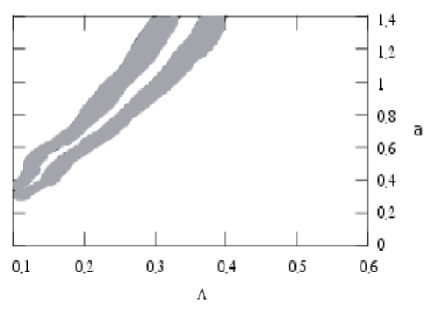
Figure 2: Space of the parameters $(a,\Lambda)$ for the theory defined by $\alpha(\varphi)=a\varphi^{2}$ and $V(\varphi)=\Lambda^{2}\varphi^{4}$ with fixed initial conditions: $\varphi_{i}=-1.3$ and $\dot{\varphi}_{i}=0$. The acceptable theories are represented by the shaded regions.

The dynamics of the scalar field and of the speed-up factor are respectively shown in figures (3) and (4) for the particular choice $(a,\Lambda)=(1,0.3\mbox{ s}^{-1})$. In a first phase, the self-interaction plays no role and the field is almost constant until $T\sim 5\mbox{ MeV}$, leading to an expansion slower than in General Relativity. Then, the $\varphi^{4}$ term starts to dominate the effective potential and attracts the scalar field towards zero. The expansion factor also oscillates and is driven to values greater than those obtained in General Relativity. The primordial abundances predicted in this case are $\mbox{Y}_{p}=0.2449$, $\mbox{D/H}=3.030\times 10^{-5}$ and ${}^{7}\mbox{Li/H}=2.387\times 10^{-10}$, in agreement with observations.

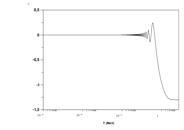
Figure 3: Evolution of the scalar field $\varphi$ during BBN for the scalar tensor theory defined by $\alpha(\varphi)=\varphi^{2}$ and $V(\varphi)=0.3^{2}\varphi^{4}$ with $\varphi_{i}=-1.3$ and $\dot{\varphi}_{i}=0$.

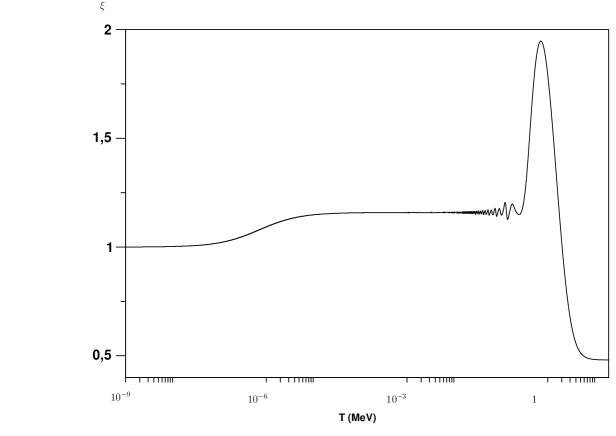
Figure 4: Speed-up factor as a function of the temperature for the scalar tensor theory defined by $\alpha(\varphi)=\varphi^{2}$ and $V(\varphi)=0.3^{2}\varphi^{4}$ with $\varphi_{i}=-1.3$ and $\dot{\varphi}_{i}=0$. The speed-up factor converges towards $1$ as soon as the matter-radiation equality is reached.

The clues for the success of this kind of scalar-tensor theories in solving the lithium problem have been already advanced at the beginning of this subsection. The evolution of the ($n/p$) ratio, as well as that of the ⁴He overproduction in the scalar-tensor model exemplified here, are shown in figure (5). As can be noticed on that figure, the effect of the speed-up factor on the n/p ratio is an integrated effect at temperatures between a few MeV and a few hundreds of keV. The fact that the speed-up factor is less than 1 at temperatures higher than 1 MeV implies that the n/p ratio departs from thermal equilibrium slighly later than in General Relativity, and this effect is partly compensated by a speed-up factor greater than one after 1 MeV, resulting in a n/p ratio that decreases faster in General Relativity than in the scalar-tensor model between 1 MeV and 0.1 MeV. These two effects almost compensate each other and result in a n/p ratio at the beginning of BBN comparable in the two models, and so, in a ⁴He abundance in the scalar-tensor model that is not very different from the one obtained in General Relativity. During the whole BBN period, the speed-up factor is instead significantly higher than unity. Then, the burning of ⁴He to produce heavier elements is less efficient than in General Relativity, and the resulting final ⁷Li abundance is low enough to be consistent with the observed value. Indeed, the reaction ${}^{3}\mbox{He}(\alpha,\gamma)^{7}\mbox{Be}$ dominates the creation of ⁷Be (and then of ⁷Li by $\beta$-decay of ⁷Be) during BBN. Therefore, neglecting the destruction of ⁷Be through the reaction ${}^{7}\mbox{Be}(\mbox{n,p})^{7}\mbox{Li}$ that is inefficient because of the low neutron abundance, a rough estimate of the final abundance of these elements can be obtained from $dY_{Be7}/dT=\Gamma Y_{He3}Y_{He4}/(TH)$ or, for small variations:

$$\Delta Y_{Be7}=\frac{\Gamma}{H}Y_{He3}Y_{He4}\Delta\ln T\$$ (34)

where $\Gamma$ is the reaction rate of ${}^{3}\mbox{He}(\alpha,\gamma)^{7}\mbox{Be}$, while $Y_{Be7}$, $Y_{He3}$ and $Y_{He4}$ denote the abundances of ⁷Be, ³He and ⁴He, respectively.

The lower panel of figure 5 shows the evolution of the ⁷Be+⁷Li abundance in this scalar-tensor model as well as in General Relativity (GR). It can be seen from this figure that both predictions start to significantly deviate only at temperatures smaller than $0.06\mbox{ MeV}$, and reach their final constant values at about $T\sim 0.03\mbox{ MeV}$. By applying the equation (34) within such a small range of temperatures, we have:

$$\frac{\Delta Y_{Be}}{\Delta Y_{Be}^{GR}}\sim\xi^{-1}\frac{Y_{He3}Y_{He4}}{Y_{He3}^{GR}Y_{He4}^{GR}},$$ (35)

that also provides an estimate of the final $Y_{Li7}/Y_{Li7}^{GR}$ ratio. At temperatures below $0.06\mbox{ MeV}$, the abundances of ³He and ⁴He are constant in both models, with $Y_{He3}\sim Y_{He3}^{GR}$ and $Y_{He4}\sim Y_{He4}^{GR}$, while the speed-up factor oscillates around $\xi\sim 1.16$. Therefore, equation (35) implies $Y_{Li7}\sim 0.8Y_{Li7}^{GR}$, in rough agreement with our result obtained from the full integration of the nuclear reaction network: $Y_{Li7}=0.74Y_{Li7}^{GR}$.

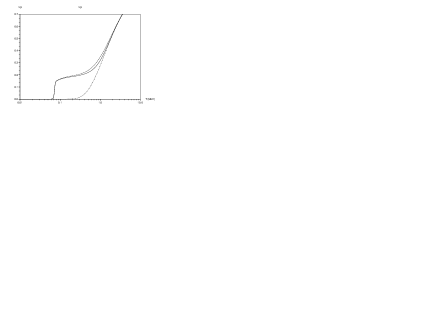
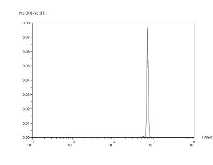
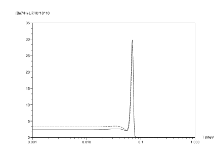
Figure 5: Upper panel: Evolution of (n/p) as a function of the temperature in General Relativity (dashed line) and in the same model as in Figure 4 (solid line). The dashed dotted line represents the (n/p) ratio at equilibrium. Medium panel: Evolution of the difference between ⁴He abundances in General Relativity and in the same model as in Figure 4. Lower panel: Evolution of the abundance of ⁷Be+⁷Li as a function of temperature in General Relativity (dashed line) and in the same model as in Figure 4 (solid line).

Of course, other theories with a different coupling function and/or a different potential could have the same effect on the ⁷Li abundance, provided that they lead to a speed-up factor with a time evolution similar to that found in the models analyzed in this section. As an example, the Appendix shows that, when the $\dot{\varphi}_{init}=0$ condition is relaxed in scalar tensor theories without a self-interaction term (then, the convergence towards General Relativity is not ensured, and requires additional conditions), some of the resulting models can also solve the lithium problem. Therefore, the mechanism found here, based on a specific shape of the variation of the expansion rate during BBN, can be achieved in a great variety of scalar-tensor cosmological models.

3.2.2 Beyond BBN processes: effects on CMB and matter power spectrum

It is important to note that, in the analysis of the previous subsection, at the end of BBN, $\alpha(\varphi)<10^{-5}$ and $A(\varphi)\sim 1$, so that $G_{eff}/G_{N}\sim 1$; moreover, $\alpha(\varphi)$ goes on decreasing because $\varphi$ decreases, so that one can consider that gravitation is indistinghishable from General Relativity already at the end of BBN. Nevertheless, the scalar field still has a non negligible energy density, and consequently, the expansion rate is not the one of General Relativity with matter dust and radiation fluids, but receives an additional contribution from the scalar field energy density. This is why the speed-up factor is not immediately $1$ but oscillates around a value of $1.16$ until the end of the radiation dominated era and converges towards 1 when dust matter begins to dominate. As a consequence, we expect that such a model will have some impact on observables such as the matter power spectrum or the CMB. This is actually the case, but, these impacts are really of a different nature that the ones that were previously investigated in the context of scalar-tensor theories (Chen & Kamionkowski, 1999; Baccigalupi & al, 2000; Torres, 2002; Nagata & al, 2002, 2003): these works address the effects of modification of gravity (mainly variations of the gravitational coupling) on the CMB and matter power spectrum. In the models presented in this paper, the variation of the gravitational coupling plays a very important role during BBN (as examplified above), well before the matter dominated era, but at the epoch of matter-radiation equality, the gravitational coupling no longer significantly varies, and the scalar field behaves almost like a standard scalar field ($\alpha(\varphi)\sim 0$). Let’s know consider the impact of our model on the matter power spectrum and on the CMB. The matter power spectrum turn-over is defined by the scale entering the Hubble horizon at the matter radiation equality (that is $H_{eq}^{-1}$) (Coble & al, 1997). Since the expansion rate is slightly faster in the model presented here than in General Relativity at the time of equality, we expect a shift in the turn over given by (Baccigalupi & al, 2000):

$$\frac{\delta k_{T}}{k_{T}}=-\left(\frac{\delta H^{-1}}{H^{-1}}\right)_{eq}\mbox{, }$$ (36)

Which yields, if we define the speed-up factor at equality by $\xi_{eq}$:

$$\frac{\delta k_{T}}{k_{T}}=\xi_{eq}-1\mbox{.}$$ (37)

With $\xi_{eq}\sim 1.075$, one then has: $\delta k_{T}/k_{T}\sim 7.5\%$. This small shift is completely compatible with the current incertainties on data (Tegmark & al, 2006).

The position of the first acoustic peak in the CMB power spectrum is also affected. The acoustic oscillations occur at an angular scale proportional to the size of the CMB sound horizon at decoupling and inversely proportional to the comoving distance between the observer and the last scattering surface. So, if one defines the conformal time:

$$\tau=\int_{0}^{t}\frac{dt}{a(t)}\mbox{, }$$ (38)

the multipole moment associated with the first peak is given by:

$$l_{p}\propto\frac{\tau_{0}-\tau_{dec}}{\tau_{0}}$$ (39)

where $\tau_{0}$ is the conformal time of the observer (today), and $\tau_{dec}$ the conformal time at decoupling. Then the shift in the position of the first peak: $\delta l_{p}/l_{p}=(l_{p}-l_{p}^{GR})/l_{p}^{GR}$ can be numerically inferred from the simulation. For the model presented above, one finds: $\delta l_{p}/l_{p}\sim 8\%$. This is a rather important shift (Page & al, 2003), but it should be stressed that it depends strongly on the value of the expansion rate today, and that it has been assumed, to make a significant comparison that this expansion rate today was the same in the two models (General Relativistic cosmology and scalar-tensor cosmology). It is possible to play with the acceptable value of $H_{0}$ (that is to give different values of $H_{0}$ to the two models) to make this shift smaller.

Finally, one expects that the model presented above will lead to other distortions in the CMB power spectrum at small scales since the expansion rate is different from the one of General Relativity during the whole radiation dominated era, when the small scales (those smaller than the one of the firsts acoustic peak) are entering the sound horizon, but investigating these problem demands a detailed analysis of the CMB physics in this new context that is beyond the scope of this paper, and will be dealt with in a forthcoming paper.

4 Conclusion

In the framework of the standard BBN, the WMAP measurement of the baryon density of the Universe $\Omega_{b}h^{2}=0.0224\pm 0.0009$ leads to a serious discrepancy between the predicted and observed ⁷Li abundance, even when systematic errors are cautiously taken into account. We addressed this problem by renewing the standard BBN scenario in a simple way: by considering that gravitation is described by a scalar-tensor theory. The expansion of the Universe during BBN is then modified, then modifying the conditions and the efficiency of nuclear reactions while assuming the standard nuclear physics. We showed that it is possible to obtain a small enough ⁷Li abundance and, at the same time, to preserve the ⁴He and D abundances thanks to a scalar-tensor theory of gravity with a non monotonic speed-up factor that has a generic behavior. The expansion must be similar to that found in General Relativity at $T\sim 1-2$MeV, so that the freezing-out temperature of the weak processes $n+\nu_{e}\leftrightarrow p+e^{-}$ and $n+e^{+}\leftrightarrow p+\bar{\nu}_{e}$ is also similar to that obtained in General Relativity, then leading to almost the same ⁴He production. However, during BBN, the expansion must be faster than in General Relativity, making the reaction ${}^{3}\mbox{He}(\alpha,\gamma)^{7}\mbox{Be}$ less efficient to burn ⁴He and to produce ⁷Li.

Consequently, the ⁷Li abundance obtained for the baryon density inferred from WMAP could be a good imprint for the presence of a scalar field explicitly coupled to matter at the beginning of the Universe, challenging our understanding of the primordial Universe and the nature of gravity at early epochs. It could then be valuable to study the possible signatures of this scalar field in inflationary scenarios and to perform a detailled analysis of its impact on CMB physics and structure formation.

Aknowledgments

We would like to thank Pr. G. Steigman for valuable comments on this work.

APPENDIX: Varying speed-up factor in theories without a self-interaction term

All the models analyzed in this paper starts from $\dot{\varphi}_{init}=0$. As a consequence, in any theory without a self-interaction term, the scalar field has a constant value during the whole radiation-dominated period. Nevertheless, previous works (Alimi & Sena, 1997; Navarro & al, 2002) have shown that, when the condition $\dot{\varphi}_{init}=0$ is relaxed, many of these theories also imply a non-monotonic evolution of the speed-up factor. The convergence of these theories towards General Relativity has instead important differences with respect to that found for the models analyzed in this paper. In non-monotonic scalar-tensor theories without a self-interaction term, the convergence towards General Relativity is not ensured independently of the initial conditions.

One of the main conclusions of this paper is that the lithium problem can be solved in many scalar-tensor theories, defined by different coupling functions and/or different potentials, but implying an evolution of the speed-up factor with the same general properties as those found in Section 3.2. In this Appendix, we explore the impact on BBN of a theory defined, in the Dicke-Jordan frame, by

$$3+2\omega(\phi)=\frac{a}{|\phi-1|}+b$$ (40)

with $\phi_{init}>1$ (this is a necessary condition for the speed-up factor to be less than unity at the beginning).

In the limit close to general relativity ($\phi\rightarrow 1$), the above theory leads (Serna & al, 2002; Barrow & Parsons, 1997) to an Einstein frame formulation with $\alpha(\varphi)\propto|\varphi|^{1/2}$ and $\varphi_{init}<0$. The effective potential defined in (19) then becomes

$$V_{eff}(\varphi)=\mbox{sgn}(\varphi)\frac{2(1-3w_{b})}{3}|\varphi|^{\frac{3}{2}},$$ (41)

where sgn$(x)=-1,0,1$ if $x$ is negative, zero or positive, respectively. This effective potential does not have a minimum, but a stationary point at $\varphi=0$. So, if the scalar field does not have a high enough initial velocity, it will roll down its effective potential during the matter-dominated era, pushing the theory far from General Relativity. Then, in these theories, one must give an initial velocity to the scalar field so that it can reach the opposite side of the stationary point $0$ before the matter dominated era. In Damour & Nordvedt (1993), it was shown that, during the radiation dominated era, the total displacement of the scalar fields is given by:

$$\Delta\varphi=\frac{\sqrt{3}}{2}ln\left(\frac{1+\varphi_{i}^{{}^{\prime}}/\sqrt{3}}{1-\varphi_{i}^{{}^{\prime}}/\sqrt{3}}\right)$$ (42)

So that we can deduce the initial velocity necessary to reach $0$, starting from $\varphi_{i}$. It is given by:

$$\varphi_{i}^{{}^{\prime}}=\sqrt{3}\frac{exp(-2)\varphi_{i}/\sqrt{3}-1}{1+exp(-2)\varphi_{i}/\sqrt{3}}$$ (43)

that is always finite and bounded by $-\sqrt{3}$ and $\sqrt{3}$.

Since it is not possible to perform the analytical transformation (2.1) to find its exact form in the Einstein frame, the models defined by (40) have been integrated in the Dicke-Jordan frame. Moreover, the integration was performed backward in time, then replacing the initial condition on the scalar field by the present value of the coupling function $\omega(\phi)$. The present value of the derivative of the scalar field was fixed to zero.

By varying the three remaining parameters $(a,b,\omega(\phi_{0}))$, we identified the cosmological models that lead to the observed abundances of light elements. The results were not sensitive to $\omega(\phi_{0})$ as long as $\omega(\phi_{0})$ is sufficiently large to pass the Solar System tests. Then, restricting the analysis to the parameters $a$ and $b$, the figure (6) shows (as shaded regions) the $(a,b)$ couples leading to primordial abundances of ⁴He, D and ⁷Li compatible with observations. Again, the two distinct admissible regions are related to the two different observations considered for the ⁴He abundance Luridiana & al (2003); Izotov & al (1999).

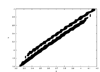
Figure 6: Acceptable theories are represented by the shaded regions in the $(a,b)$ plane, for $3+2\omega(\phi)=\frac{a}{|\phi-1|}+b$ in the Dicke-Jordan frame.

Figure 7: Speed-up factor as a function of the temperature (in MeV) during BBN.

As an illustration of these theories, the figure (7) shows the evolution of speed-up factor corresponding to the particular choice $a=4$, $b=2.68$ and $\omega(\phi_{0})=10^{14}$. It exhibits the behavior we described previously in order to solve the lithium problem and to preserve the ⁴He abundance. The predicted primordial abundances in this example were in fact: $\mbox{Y}_{p}=0.2405$, $\mbox{D/H}=2.871\times 10^{-5}$ and ${}^{7}\mbox{Li/H}=2.601\times 10^{-10}$.

References

- Angulo & al (1999) Angulo, C. & al 1999, Nucl. Phys. A, 656, 3
- Asplung & al (2005) Asplund, M., Lambert, D., Nissen, P., Primas, F., & Smith, V. 2005, astro-ph/0510636, submitted to Astrophys. J.
- Baccigalupi & al (2000) Baccigalupi, C., Matarrese, S., & Perrotta, F. 2000, Phys. Rev. D, 62, 123510
- Barrow (1978) Barrow, J. 1978, Non. Not. R. Astron. Soc., 184, 677
- Barrow & Parsons (1997) Barrow, J., & Parsons, P. 1997, Phys. Rev. D, 55, 1906
- Beaudet & Yahil (1977) Beaudet, G., & Yahil, A. 1977, Astrophys. J., 218, 253
- Bennett & al (2003) Bennett, C. & al 2003, Astrophys. J. S., 148, 1
- Bergmann (1968) Bergmann, P. 1968, Int. J. Theor. Phys., 1, 25
- Bonifacio & al (2002) Bonifacio, P. & al 2002, Astron. Astrophys., 390, 91
- Boesgaard & al (2005) Boesgaard, A.M., Novicki, M., & Stephens, A. 2005, Proceedings IAU Symposium No. 228, Hill, V., Fran ois, P., & Primas, F. eds 2005, astroph/0509653
- Brans & Dicke (1961) Brans, C., & Dicke, R. 1961, Phys. Rev., 124, 925
- Caughlan & Fowler (1998) Caughlan, G., & Fowler, W. 1988, AT. DATA Nucl. Data Tables, 40, 291
- Chen & Kamionkowski (1999) Chen, X., & Kamionkowski, M. 1999, Phys. Rev. D, 60, 104036
- Clifton & al (2005) Clifton, T., Barrow, J., & Scherrer, R. 2005, Phys. Rev. D, 71, 123526
- Coble & al (1997) Coble, K., Dodelson, S., & Friemann 1997, Phys. Rev. D, 55, 1851
- Coc & al (2004) Coc, A., Vangioni-Flam, E., Descouvemont, P., Adahchour, A., & Angulo, C. 2004, Astrophys. J., 600, 544
- Coc & al (2006) Coc, A., Olive, K., Uzan, J.P., & Vangioni, E. 2006, Phys. Rev. D, 73, 083525
- Cyburt & al (2003) Cyburt, R., Fields, B., & Olive, K. 2003, Phys. Lett. B, 567, 227
- Cyburt (2004) Cyburt, R. 2004, Phys. Rev. D, 70, 023505
- Damour & Nordvedt (1993) Damour, T., & Nordtvedt, K. 1993, Phys. Rev. D, 48, 3436
- Ellis & al (2005) Ellis, J., Olive, K., & Vangioni E. 2005, Phys. Lett. B, 619, 30-42
- Green & al (1988) Green, M., Schwarz, J., & Witten E. 1988, Superstring Theory, Cambridge University Press
- Ichikawa & al (2004) Ichikawa, K., Kawasaki, M., & Takahashi, F. 2004, Phys.Lett.B, 597, 1-10
- Izotov & al (1999) Izotov, Y. & al. 1999, Astrophys. J., 527, 757
- Jedamzik & Rehm (2001) Jedamzik, K., & Rehm, J.B. 2001, Phys. Rev. D, 64, 023510
- Jedamzik1 (2004) Jedamzik, K. 2004, Phys. Rev. D, 70, 063524
- Jedamzik2 (2004) Jedamzik, K. 2004, Phys. Rev. D, 70, 083510
- Kirkman & al (2003) Kirkman, D., Tyler, D., Suzuki, N., O’Meara, J., & Lubin 2003, D., Astrophys. J. S., 149, 1
- Kneller & Steigman (2004) Kneller, J. P., & Steigman G. 2004, New Journal of Physics, 6, 117
- Luridiana & al (2003) Luridiana, V. & al. 2003, Astrophys. J., 592, 846
- Nagata & al (2002) Nagata, R., Chiba, T., & Sugiyama, N. 2002, Phys.Rev. D, 66, 103510
- Nagata & al (2003) Nagata, R., Chiba, T., & Sugiyama, N. 2003, Phys.Rev. D, 69, 083512
- Navarro & al (2002) Navarro, A., Serna, A., & Alimi, J.-M. 2002, Class. Quantum Grav., 19, 4361-4375
- Nordvedt (1970) Nordvedt, K. 1970, Astrophys. J., 161, 1059
- Page & al (2003) Page, L., et al. 2003, Astrophys. J. S., 148, 233
- Ryan & al (2000) Ryan, S. & al 2000, Astrophys. J., 530, L57
- Ryan & al (1999) Ryan, S., Norris, J., & Beers, T. 1999, Astrophys. J., 523, 654
- Serna & Alimi (1996) Serna, A., & Alimi, J.-M. 1996, Phys. Rev. D, 53, 3087
- Alimi & Sena (1997) Alimi, J.-M., & Serna, A. 1997, Astrophys. J., 487, 38
- Serna & al (2002) Serna, A., Alimi, J.-M., & Navarro, A. 2002, Class. Quantum Grav., 19, 857-874
- Smith & al (1993) Smith, M., Kawano, L., & Malaney, R. 1993, Astrophys. J. S., 85, 219
- Spergel & al (2003) Spergel, D. & al. 2003, Astrophys. J. S., 148, 175
- Tegmark & al (2006) Tegmark, M., et al. 2006, astro-ph/0608632
- Thevenin & al (2001) Thevenin, F. & al 2001, Astron. Astrophys., 373, 905
- Torres (2002) Torres, D. 2002, Phys. Rev. D, 66, 043522
- Wagoner (1970) Wagoner, R. 1970, Phys. Rev. D, 1, 3209
- Wagoner (1973) Wagoner, R. 1973, Astrophys. J., 179, 343