Microlensing of Circumstellar Envelopes

This paper examines line profile evolution due to the linear expansion of circumstellar material obsverved during a microlensing event. This work extends our previous papers on emission line profile evolution from radial and azimuthal flow during point mass lens events and fold caustic crossings. Both “flavours” of microlensing were shown to provide effective diagnostics of bulk motion in circumstellar envelopes. In this work a different genre of flow is studied, namely linear homologous expansion, for both point mass lenses and fold caustic crossings. Linear expansion is of particular relevance to the effects of microlensing on supernovae at cosmological distances. We derive line profiles and equivalent widths for the illustrative cases of pure resonance and pure recombination lines, modelled under the Sobolev approximation. The efficacy of microlensing as a diagnostic probe of the stellar environs is demonstrated and discussed.

1 Introduction

Recently gravitational microlensing has been shown to be a powerful tool for probing not only the nature and distribution of dark matter but also the astrophysical properties of the source being lensed (see, for example, Gould 2001 for a comprehensive review). While the vast majority of microlensing events observed to date can be adequately approximated as point sources lensed by a point mass lens, there is a small but significant fraction of events in which the source must be modelled as extended, which has important consequences for the evolution of the broad-band lightcurve and spectrum during the microlensing event and produces observational signatures that are now readily detectable – chiefly due to the introduction of microlensing ‘alert’ networks. This development has allowed intensive photometric and spectroscopic monitoring of many microlensing events, spearheaded by the PLANET collaboration (Albrow et al. 1998). The alert strategy is especially well-suited to fold caustic crossings – in e.g. close binary lensing events – since observation of the first caustic crossing permits prediction of the second caustic crossing, allowing intensive follow-up observations to be scheduled. Moreover, every fold caustic crossing must be treated as an extended source event, making them ideal probes of the astrophysics of the source.

In the past few years ‘alert response’ broad-band photometric observations of extended source microlensing events have shown clear detections of stellar limb darkening on the photospheres of a number of stars, including: K giants (Albrow et al. 1999; Albrow et al. 2000; Fields et al 2003), a metal-poor A dwarf in the Small Magellanic Cloud (Afonso et al. 2000), a G/K subgiant (Albrow et al. 2001a) and an F8-G2 solar-type star (Abe et al. 2003). These observations have been used to estimate limb darkening parameters and to constrain stellar atmosphere models, comparing for example the LTE ATLAS models of Kurucz (1994) with the PHOENIX ‘Next Generation’ models of Hauschildt et al. (1999).

In addition Albrow et al. (2001b) used the VLT to carry out observations of $H\alpha$ equivalent width variation in the atmosphere a K3 bulge giant during a fold caustic crossing event. These authors showed that highly resolved observations of the microlensed spectrum could be a powerful discriminant between different stellar atmosphere models, and indeed could also be a useful method for breaking the near-degeneracy between the parameters of different lens models. This work essentially vindicated the theoretical modelling of Heyrovský, Sasselov and Loeb (2000), which predicted that with 8m-class telescopes it should be possible to use highly time- and spectrally-resolved observations of microlensing events to carry out ‘tomography’ of stellar atmospheres.

A notable feature of the theoretical literature on extended source microlensing events, however, has been the comparative neglect of extended circumstellar envelopes. Although the model developed in Coleman (coleman1998 (1998)) and Simmons et al. (2002) includes such a scattering envelope, and Coleman et al. (1997) also considered the case of a non-spherical envelope (e.g., a Be disk), these computations were carried out only for the broad-band photometric and polarimetric response to a microlensing event.

In two preceding papers, Ignace & Hendry (1999) and Bryce, Ignace and Hendry (2003) calculated the microlensing signatures of emission line profiles from expanding and rotating spherical shells, lensed by a point mass lens and a fold caustic respectively. Their results were for highly simplistic velocity fields – constant expansion or constant rotation – in order to isolate the effects of the microlensing and demonstrate clearly the diagnostic potential for deriving velocity information about the shells. The authors showed that, while in the absence of lensing the integrated line profiles for expanding and rotating shells yielded identical ‘flat top’ profiles in each case, microlensing clearly breaks the degeneracy between these cases.

In this third paper, we choose to focus on the particular case of circumstellar media in homologous expansion, with radial velocity $v(r)\propto r$. This case is interesting for two reasons. Firstly, this type of velocity law applies to the early phases of nova and supernova (SN) explosions. Since the latter are observed to cosmological distances, it becomes increasingly likely that such events will be lensed as the light from the SN makes its way from a distant galaxy to the Earth (c.f. Dalal et al. 2003). Thus a consideration of homologous expansion is relevant if only to investigate definite signatures of microlensing from emission profile shapes observed in SN events. Indeed Bagherpour et al. (2004) consider the microlensed lightcurves of Type Ia SN, and Bagherpour et al. (2005) extend their analysis to consider the impact of microlensing on P Cygni profiles in the spectra of Type Ia SN.

Secondly, in this paper we employ standard Sobolev theory to model the emission line profiles; the Sobolev approximation is valid for the highly supersonic flows commonly found in SNe and stellar winds. Furthermore the case of homologous expansion leads to a significant simplification of the expressions and a consequent substantial reduction in computational effort. Thus it is worthwhile studying this case to better appreciate the characteristics of how microlensing will affect emission lines formed in winds with more general velocity laws.

The structure of this paper is as follows. In Section 2 we describe the basic features of line formation theory, and the Sobolev approximation which we employ. In Section 3 we derive, and briefly discuss, unlensed profiles for the case of pure resonance and pure recombination lines, in a stellar wind undergoing homogolous expansion. In Section 4 we present illustrative results, calculating the time evolution of line profile and equivalent width for pure resonance and pure recombination lines lensed by a point mass lens and a fold caustic. Finally in Section 5 we discuss our results and their future applicability in a number of specific astrophysical contexts.

2 Line formation theory

We first need to derive the emission profile for the unlensed case, expressed in terms of intensity as a function of frequency and position within the envelope of circumstellar material. For an envelope in bulk motion such that the flow speed greatly exceeds the thermal broadening, the locus of points contributing to the emission at any particular frequency in the line profile is confined to an “isovelocity zone” (c.f., Mihalas mihalas1978 (1978)). These zones are determined by the Doppler shift formula, namely

$$\nu_{z}=\nu_{0}\left(1-\frac{v_{z}}{c}\right)\,,$$ (1)

where the observer’s coordinates are $(x,y,z)$ with the line-of-sight along $z$, $\nu_{\rm{z}}$ is the Doppler shifted frequency, and $v_{z}=\bf{-v(r)\cdot\hat{z}}$ is the projection of the flow velocity onto the line-of-sight (as indicated in Figures 1 and 2). Note that both Cartesian $(x,y,z)$ and spherical $(r,\vartheta,\varphi)$ coordinates can be defined for the star. Employing the Sobolev theory for line profile calculation in moving media reduces the radiation transfer in a moving envelope to a calculation in which one need consider only distinct isovelocity zones. Equation (1) will therefore prove crucial for relating the variable profile shape to the kinematics of the envelope.

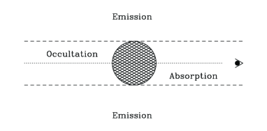
Figure 1: A schematic showing the contribution from different regions to the line profile shape, for an observer on the right hand side. Much of the line emission is produced around the circular tube indicated in projection by the dashed lines. On the far side (left hand side) of the tube the emission will be occulted by the star. On the near side, the circumstellar material will attenuate the continuum emission from the central photosphere.

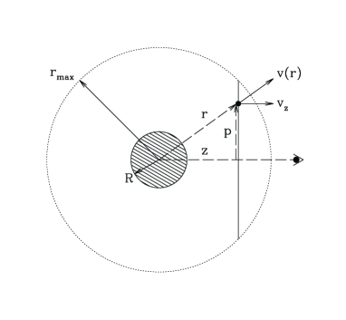
Figure 2: A schematic showing the isovelocity zones (surfaces of constant $v_{z}$) for our velocity model. These are circular plane surfaces which are oriented normal to the observer’s line-of-sight. We assume that the photosphere is of radius $R$, and the envelope is of maximum radial extent $r_{\rm max}$.

For the assumed linear expansion, and for an envelope of maximum radial extent $r_{\rm{max}}$, the velocity $\bf{v}$ at radial distance $r$ is given by

$${\bf{v}}=v_{\rm{max}}\,(r/r_{\rm{max}})\,{\bf{\hat{r}}}\,,$$ (2)

where $\bf{\hat{r}}$ is a unit vector in the radial direction and $v_{\rm{max}}$ is the wind speed at $r=r_{\rm{max}}$. The velocity shift as seen by the observer, situated as in Figure 1, is then

$$v_{z}=-v_{\rm{max}}(r/r_{\rm{max}})\,\cos\vartheta=-v_{\rm{max}}\,(z/r_{\rm{max}})\,,$$ (3)

where $\vartheta$ is the angle between the radial direction and the line of sight.

Thus isovelocity zones for constant $v_{z}$ are seen to be plane surfaces. In fact, given the spherical symmetry of our model, the isovelocity zones are circular plane surfaces of radius

$$p_{\rm{max}}=\sqrt{r_{\rm{max}}^{2}-z^{2}}\,,$$ (4)

as depicted in Figure 2.

Consider a projected element of the stellar wind at fixed impact parameter $p$, and angle $\alpha$ measured clockwise from $x$ – i.e. $x=p\cos\alpha$ and $y=p\sin\alpha$. The emergent intensity $I_{\nu}(p)$ due to emission from the wind is given by

$$I_{\nu}(p)=\int_{z}^{\infty}\,\kappa_{\nu}(r)\,\rho(r)\,S_{\nu}\,e^{-\tau_{\nu}}\,dz^{\prime}\,,$$ (5)

where $\kappa_{\nu}$ is the opacity, $\rho$ the density, $S_{\nu}$ the source function, and $\tau_{\nu}$ the optical depth at radial distance $r$, satisfying $r^{2}=p^{2}+z^{\prime 2}$.

The Sobolev approximation is to evaluate the optical depth only at the point where the Doppler shifted frequency of a gas parcel exactly equals the observed frequency. This delta function response in frequency simplifies considerably the expression for the optical depth, namely

$$\tau_{\nu}(z) = \int_{z}^{\infty}\,\kappa_{\nu}(r)\,\rho(r)\,\delta(\nu_{z}-\nu_{z^{\prime}})\,dz^{\prime}$$ (6)

$$= \frac{\kappa_{\nu}(r)\,\rho(r)\,\lambda_{0}}{|dv_{z}/dz|_{z}}\,.$$

The denominator on the right hand side is the line-of-sight velocity gradient. For a spherical flow, this gradient is given by the expression

$$\frac{dv_{z}}{dz}=\mu^{2}\,\frac{dv}{dr}+(1-\mu^{2})\,\frac{v}{r}\,.$$ (7)

For the case of homologous expansion, with $v(r)=v_{\rm max}\,(r/r_{\rm max})$, the line-of-sight velocity gradient simplifies to $dv_{z}/dz=v_{\rm max}/r_{\rm max}$, which is a constant. Therefore, although the Sobolev optical depth will generally depend on angle $\vartheta$ through the factor $dv_{z}/dz$, homologous expansion is the single exception for which the optical depth depends on radius only. The optical depth is now

$$\tau_{\nu}(r)=\frac{\kappa_{\nu}(r)\,\rho(r)\,\lambda_{0}\,r_{\rm max}}{v_{\rm max}}\,.$$ (8)

Knowing the optical depth as a function of $r$, we can then obtain an expression for the intensity, $I_{\nu}(p)$, using equations (4) and (6) and the equation

$$p^{2}=r^{2}-z^{2}\,.$$ (9)

In Sobolev theory the intensity then reduces to the form

$$I_{\nu}(p)=S_{\nu}(r)\,\left(1-e^{-\tau_{\nu}(r)}\right)\,.$$ (10)

Allowing for line emission from resonance line scattering and collisional de-excitation, and defining $\epsilon$ as the ratio of the collisional de-excitation rate to that of spontaneous decay, the source function can be derived to be

$$S_{\nu}=\frac{\beta_{\rm c}\,I_{*,\nu}+\epsilon\,B_{\nu}}{\beta+\epsilon}\,.$$ (11)

The two parameters $\beta_{\rm c}$ and $\beta$ are respectively the penetration and escape probabilities, which are given by

$$\beta_{\rm c}=\frac{1}{4\pi}\,\int_{\Omega_{*}}\,\frac{1-e^{-\tau_{\nu}}}{\tau_{\nu}}\,d\Omega\,,$$ (12)

and

$$\beta=\frac{1}{4\pi}\,\int_{4\pi}\,\frac{1-e^{-\tau_{\nu}}}{\tau_{\nu}}\,d\Omega\,,$$ (13)

where $\Omega_{*}$ is the solid angle subtended by the star at radius $r$.

The optical depth is generally anisotropic, but as already noted for homologous expansion the optical depth is isotropic in this special case. As a result, the penetration and escape probabilities are easily calculable, and in particular $\beta_{\rm c}=W(r)\,\beta$, where the dilution factor

$$W(r)=0.5\,(1-\sqrt{1-R^{2}/r^{2}})\,.$$ (14)

So for linear expansion, we have the well-known result that the Sobolev optical depth is a function of radius only. Since the source function also depends only on radius (or equivalently on impact parameter, $p$, at fixed $v_{z}$), so too does the intensity. To compute the total emergent flux at a given Doppler shift in the line profile due to emission in the circumstellar envelope, we must integrate over emergent intensity beams as given by

$$F_{\nu}(v_{z})=\frac{1}{D^{2}}\,\int_{v_{z}}\,I_{\nu}(p)\,p\,dp\,d\alpha\,,$$ (15)

where $D$ is the distance from the Earth. Substituting in for the intensity, the integration for the flux becomes

$$F_{\nu}(v_{z})=\frac{2\pi}{D^{2}}\,\int_{p_{\rm min}}^{p_{\rm max}}\,S_{\nu}(r)\,\left(1-e^{-\tau_{\nu}(r)}\right)\,p\,dp\,.$$ (16)

where we have, of course, performed the (trivial) integral over the angle $\alpha$, and the limits $p_{\rm min}$ and $p_{\rm max}$ are discussed below. For homologous expansion we know that the Sobolev surfaces are disks oriented transverse to the line-of-sight (i.e., with $z={\rm constant}$). From equation (9) this means that $pdp=rdr$, and so the above flux integral could be equivalently re-formulated as

$$F_{\nu}(v_{z})=\frac{2\pi}{D^{2}}\,\int_{r_{\rm min}}^{r_{\rm max}}\,S_{\nu}(r)\,\left(1-e^{-\tau_{\nu}(r)}\right)\,r\,dr\,.$$ (17)

We now include the contribution of continuum radiation from a pseudo-photosphere at radius $R$. It is instructive to consider separately redshifted and blueshifted wavelengths, which correspond to $v_{z}>0$ and $v(z)<0$ respectively.

For $v(z)>0$ (the redshifted side) the total flux $F_{\rm tot}(v_{z})$ at frequency $\nu$ and line-of-sight velocity $v_{z}$ may be written as

$$F_{\rm tot}(v_{z})=F_{1}(v_{z})+F_{2}(v_{z})\,,$$ (18)

where

$$F_{1}(v_{z})=\frac{2\pi}{D^{2}}\,\int_{0}^{R}\,I_{\rm phot}\,\,p\,dp\,,$$ (19)

and

$$F_{2}(v_{z})=\frac{2\pi}{D^{2}}\,\int_{R}^{p_{\rm max}}\,S_{\nu}(r)\,\left(1-e^{-\tau_{\nu}(r)}\right)\,p\,dp\,.$$ (20)

Here $I_{\rm phot}$ is the continuum intensity of the pseudo-photosphere. If $I_{\rm phot}$ is a constant then the integrals involving $I_{\rm phot}$ become very straightforward. $F_{1}$ represents the flux coming directly from the pseudo-photosphere while $F_{2}$ accounts for photons scattered by the surrounding envelope which emerge along the line of sight. Note that the lower limit of the $F_{2}$ integral is $R$ since the region for $p<R$ is occulted by the pseudo-photosphere of the star. The upper limit, $p_{\rm max}$ satisfies the relation

$$p_{\rm max}^{2}=r_{\rm max}^{2}-z^{2}\,.$$ (21)

For $v(z)<0$ (the blueshifted side) the total flux consists of three terms, i.e.

$$F_{\rm tot}(v_{z})=F_{3}(v_{z})+F_{4}(v_{z})+F_{5}(v_{z})\,,$$ (22)

where

$$F_{3}(v_{z})=\frac{2\pi}{D^{2}}\,\int_{0}^{p_{\rm lim}}\,I_{\rm phot}\,\,p\,dp\,,$$ (23)

$$F_{4}(v_{z})=\frac{2\pi}{D^{2}}\,\int_{p_{\rm lim}}^{p_{\rm max}}\,S_{\nu}(r)\,\left(1-e^{-\tau_{\nu}(r)}\right)\,p\,dp\,,$$ (24)

and

$$F_{5}(v_{z})=\frac{2\pi}{D^{2}}\,\int_{p_{\rm lim}}^{R}\,I_{\rm phot}\,e^{-\tau_{\nu}(r)}\,p\,dp\,.$$ (25)

Here $p_{\rm lim}$ is defined as

$$p_{\rm lim}=\left\{\begin{array}[]{ll}\sqrt{R^{2}-z^{2}}&\quad{\rm for}\,\,0\leq z\leq R\\ 0&\quad{\rm for}\,\,z>R\end{array}\right.\quad.$$ (26)

Note that if $z>R$ then the $F_{3}$ integral is identically zero; in this case the flux contribution from the pseudo-photosphere is represented fully by the $F_{5}$ term, which also takes account of attenuation by intervening wind material along the line-of-sight.

Finally we must stress that, in accordance with the standard notation adopted in the microlensing literature, all distance scales are in fact taken as angular distances that are normalised to the angular Einstein radius of the lens. This implies that the “fluxes” defined in the above equations have rather unusual units. however, the results of our line profile calculations in the following sections will be displayed as ratios normalised by the continuum, so that the (non-standard) units of flux will cancel.

3 Unlensed profiles from homologous expansion

Before including the effects of gravitational lensing we first consider the unlensed profiles derived by applying the model of the previous section to the illustrative cases of a pure resonance line and a pure recombination line. We have computed line profiles for a range of optical depths, assuming a spherically symmetric density distribution for the ejecta given by

$$\rho(x)=\rho_{0}\,x^{-3}\,,$$ (27)

where $x=r/R$. The factor $x^{-3}$ accounts for mass continuity within the shell as material expands. The scale parameter $\rho_{0}$ denotes the density at the radius of the pseudo-photosphere and specifies the total amount of gas ejected in the explosion, via the equation

$$M_{\rm ejecta}=\int\,4\pi r^{2}\,\rho(r)\,dr\,.$$ (28)

3.1 Pure resonance lines

For the case of a pure resonance line the parameter $\epsilon$ is set to zero in eq. (11), and the source function becomes

$$S_{\nu}=W(r)\,I_{*,\nu}\,.$$ (29)

The opacity for resonance line scattering does not depend explicitly on density, but an implicit dependence can arise through, for example, the ionization fraction of whatever atomic species is being considered. For simplicity, we suppress any radial dependence of the opacity in our model, and parametrize the Sobolev optical depth as

$$\tau_{\nu}=\tau_{0}\,(\rho/\rho_{0})=\tau_{0}\,x^{-3}\,.$$ (30)

An especially convenient parameter used to characterize different line calculations is the line integrated optical depth defined as follows

$${\rm T}=\int^{x_{\rm{max}}}_{1}\,\tau_{\nu}\,dx\,=\,\frac{1}{2}\tau_{0}\left(1-\frac{1}{x_{\rm max}^{2}}\right)\,.$$ (31)

Thus, for fixed $x_{\rm{max}}$, it is trivial to compute the value of $\tau_{0}$ – and hence the model profile – corresponding to a given value of $\rm T$.

Figure 3 shows some examples of model profiles computed for $\rm T=0.3,1.0,3.0$ and $10.0$, with stronger lines corresponding to larger values of $\rm T$. In all cases a fixed value of $x_{\rm max}=5$ was adopted, so that from equation (31) $\rm T=0.48\tau_{0}$. Note that our chosen value of $x_{\rm max}$ is responsible for the change of slope of each line profile at $v_{z}=-0.2v_{\rm max}$. This is due to the occultation of wind material which lies directly behind the pseudo-photosphere of the star (at $x=0.2x_{\rm max}$ in this case).

Increasing the value of $x_{\rm max}$ would result in qualitatively similar line profiles but with a narrower emission peak and absorption trough. We can understand this behaviour as follows. From equations (3) and (9) we can write

$$x=\sqrt{\frac{p^{2}}{R^{2}}+w^{2}x_{\rm max}^{2}}\,\,,$$ (32)

where $w=v_{z}/v_{\rm max}$. From equation (30) it then follows that for $w\simeq 0$ the optical depth – and hence the line flux – is insensitive to $x_{\rm max}$ (The range of integration in equation (16) increases as $x_{\rm max}$ increases, but this has little effect on the line flux because the optical depth is proportional to $x^{-3}$).

For $w\simeq\pm 1$, on the other hand, at fixed $p$ the optical depth decreases sharply as $x_{\rm max}$ increases – resulting in reduced line emission and absorption and thus a narrowing of these features in the line profile.

3.2 Pure recombination lines

We have also computed model profiles for the case of a pure recombination line. As such, scattering is ignored, and the source function is assumed to arise from an LTE process, so that

$$S_{\nu}=B_{\nu}(T)\,,$$ (33)

for temperature, $T$. For simplicity, the envelope shall be taken as isothermal. The opacity for a recombination line is $\kappa\propto\rho$, and so the scaling of the optical depth will for this case be

$$\tau_{\nu}=\tau_{0}\,(\rho/\rho_{0})^{2}.$$ (34)

As a $\rho^{2}$ process, the optical depth will go as $x^{-6}$ – a strong function of radius.

It is again useful to introduce the integrated optical depth parameter given by

$${\rm T}=\int^{x_{\rm max}}_{1}\,\tau_{0}\,(\rho/\rho_{0})^{2}\,dx\,,$$ (35)

so that again, for fixed $x_{\rm max}$, it is trivial to compute the value of $\tau_{0}$ corresponding to a line of given integrated optical depth.

Figure 4 shows profile shapes again computed for $x_{\rm max}=5$ and for the same range of values of $\rm T$ as in Figure 3. From equation (35) it follows that $\rm T\approx 0.2\tau_{0}$. Note that in contrast to Figure 3, the recombination lines do not exhibit any blueshifted absorption. That is because we assume that the continuum emission is given by a blackbody with the same temperature as the envelope. Consequently for sightlines that intercept the continuum forming surface, one has $I_{\nu}=B_{\nu}e^{-\tau}+B_{\nu}(1-e^{-\tau})=B_{\nu}$. Hence the combined emission from line plus continuum will always equal or exceed the continuum level when integrated over all sightlines.

As was the case for pure resonance lines, increasing $x_{\rm max}$ would produce narrower profiles but would have negligible effect on the value of the peak emission at $w=0$ for fixed $\rm T$.

Figure 3: Model line profiles from pure resonance line scattering, calculated using the method described in the text, for four values of the integrated optical depth, $\rm T$. The stronger lines correspond to larger values of $\rm T$.

Figure 4: Model line profiles from pure recombination line scattering, calculated using the method described in the text, for four values of the integrated optical depth, $\rm T$. The stronger lines correspond to larger values of $\rm T$.

4 Lensed profiles from homologous expansion

We now consider the effect of microlensing on emission line profiles for a stellar wind in homologous expansion. Our expression in equation (15) for the emergent flux is now replaced by an integral over emergent intensity beams weighted by the (dimensionless) lensing magnification $A(d)$, where $d$ is the projected separation between the lens and an area element of the wind in the source plane, i.e.

$$F(v_{z})=\frac{1}{D^{2}}\,\int_{0}^{2\pi}\,\int_{p_{\rm min}}^{p_{\rm max}}\,I_{\nu}(p)A(d)\,p\,dp\,d\alpha\,\,.$$ (36)

Note that, while we continue to assume that $I_{\nu}$ depends only on impact parameter, the lensing magnification is a function of both $p$ and $\alpha$, so that we must perform a double integration to compute the emergent flux at each radial velocity. Moreover, since the magnification pattern of the lens evolves with time, as the relative projected positions of the lens and wind change, the computed line profile will also be time-dependent.

The form of the magnification function is determined by the nature of the lens. In this paper we consider two illustrative cases: those of a point mass lens and a fold caustic.

4.1 Point mass lensing event

In the typical microlensing situation of a point mass lens the (time-dependent) magnification factor takes the well-known form (see e.g. Pacyński 1986)

$$A(u)=\frac{u^{2}+2}{u\sqrt{u^{2}+4}}$$ (37)

where $u$ is the impact parameter: the projected separation between the lens and source element, given by

$$u(t)=\sqrt{u_{0}^{2}+\frac{(t-t_{0})^{2}}{t_{E}^{2}}}$$ (38)

where $t_{0}$ is the time of closest approach between lens and source element, which occurs at $u=u_{0}$, the minimum impact parameter, and $t_{E}$ is the characteristic timescale of the event. Both $u$ and $u_{0}$ are expressed in units of the angular Einstein radius of the lens, which is defined as

$$\theta_{E}=\sqrt{\frac{4GM}{c^{2}}\frac{D_{S}-D_{L}}{D_{S}D_{L}}}$$ (39)

where $M$, $D_{S}$, $D_{L}$ are the lens mass, source distance and lens distance respectively. The timescale $t_{E}$ may be written as

$$t_{E}=\frac{\theta_{E}}{\mu_{\rm rel}}$$ (40)

where $\mu_{\rm rel}$ is the relative proper motion of the lens.

In the limit of large separations the magnification is, of course, equal to unity while for small $u$ the magnification goes approximately as $1/u$. Thus if a point lens transits an extended source, while formally the magnification factor is infinite for the source element directly behind the lens, when one integrates over the finite area of the source an finite value for the magnification is obtained.

Figure 5 illustrates schematically the geometry of a point lens event. The outer edge of the circumstellar envelope (of radius $r_{\rm max}$) is shown in projection, together with the trajectory of the lens. When the lens is at position $L$, an area element of the wind at position $S$ (defined by polar coordinates $p$ and $\alpha$ – see eq. 36) lies a projected distance $u$ from $L$.

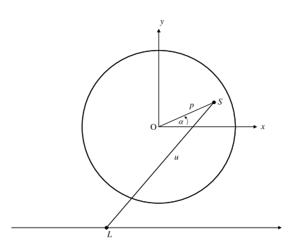
Figure 5: A schematic view of the source plane for a point lens event, showing in projection (i.e. with the observer in the $z$ direction) the outer edge of the circumstellar envelope (of radius $r_{\rm max}$) and the trajectory of the point lens, $L$. An element of the source, at $S$, with position defined by polar coordinates $p$ and $\alpha$, is shown; it lies at a projected separation $u$ from the lens.

Figure 6: The lightcurve, equivalent widths and line profiles produced by a point mass lens transiting a star with photospheric radius $R=0.03\,\theta_{E}$ surrounded by a circumstellar envelope exhibiting pure resonance line scattering. The upper left panel shows the change in apparent magnitude of the lensed continuum flux, compared with the unlensed flux, as a function of time. Below it the time evolutioin of the normalised equivalent width of the resonance line is shown. The four line profiles in the right hand panel correspond to the epochs represented by dotted vertical lines in the right hand panel. Thus, for example, profile ‘b’ corresponds to the epoch of maximum magnification (when the lens is at its minimum impact parameter) and is also when the largest change in equivalent width occurs. The solid lines in the right hand panel show the lensed line profiles while the dashed lines show the unlensed profiles, and are included for comparison. The offset between the profiles is provided for clarity. All profiles were calculated for an integrated optical depth of $T=3.0$ and assuming $x_{\rm max}=5$.

Figure 7: The lightcurve, equivalent widths and line profiles produced by a point mass lens transiting a star with photospheric radius $R=0.03\,\theta_{E}$ surrounded by a circumstellar envelope exhibiting pure recombination line scattering. The three panels present results in the same manner as in Figure 6. All profiles were again calculated for an integrated optical depth of $T=3.0$ and assuming $x_{\rm max}=5$.

4.1.1 Pure resonance lines

We computed continuum lightcurves, line equivalent widths and line profiles for the case of a pure resonance line lensed by a point mass lens. Illustrative results are shown in Figure 6 for a transit with minimum impact parameter equal to zero – i.e. assuming the lens crosses exactly over the centre of the circumstellar envelope – and adopting a photospheric radius $R=0.03\,\theta_{E}$. This value is representative of source radii determined for observed microlensing events exhibiting finite source effects. Indeed Macho event M95-30, which was the first well-documented example of a finite source event, was found to have a somewhat larger radius of $R\approx 0.075\,\theta_{E}$ (Alcock et al. 1997). In the results shown in Figure 6 we truncated the radius of the circumstellar envelope at $x_{\rm max}=5$ and the line profiles were taken to have integrated optical depth $\rm T=3$.

The upper left hand panel of Figure 6 shows the continuum lightcurve of the lensing event – i.e. the change in apparent magnitude, computed from the ratio of lensed to unlensed continuum flux, as a function of time. The time axis is measured in units of $t_{E}$ – the lensing timescale introduced in equation (40). As expected, the maximum magnitude change occurs at minimum impact parameter, when the lens transits the centre of the photosphere, and the continuum flux is boosted by a factor of more than 60. Only the central portion of the light curve is shown; although lensing still produces a continuum flux magnification of $\sim 5$ when $(t-t_{0})/t_{E}=\pm 0.2$, the effect of lensing on the line profiles is essentially negligible for larger impact parameters.

The lower left hand panel of Figure 6 shows the time evolution in the normalised equivalent width of the resonance line. The equivalent width was calculated according to the formula

$${\rm EW}=\left<\frac{F(v_{z})}{F_{\rm cont}}\right>\,-\,1\,\,,$$ (41)

where the angled brackets denote the mean, or expectation, value obtained by integrating over $v_{z}$.

The vertical dashed lines labelled a, b, c and d in the upper and lower left hand panels correspond to the four epochs in the right hand panel at which the lensed (solid curve) and unlensed (dashed curve) line profiles are compared. For clarity a constant vertical offset is introduced between each of the four epochs; note that this does not indicate any change in magnification.

We can see from the lower left panel that the unlensed value (i.e. for large impact parameter) of the the normalised equivalent width is slightly negative because of the asymmetry in the unlensed line profile: the area of the blueshifted absorption trough is slightly larger than that of the redshifted emission peak. As the event proceeds and the lens crosses the outer edge of the envelope, at $(t-t_{0})/t_{E}=-0.15$, the normalised equivalent width at first shows a clear increase, as the lens differentially magnifies a portion of the isovelocity zones in emission. This stage of the lensing event corresponds to profile (a) in the right hand panel. As the projected lens position approaches the photosphere, however, the absorption component of the line profile quickly begins to dominate. This is because the lens is differentially magnifying the attenuated continuum emission coming from the photosphere. The equivalent width reaches its lowest value when the lens has zero impact parameter – i.e. when it lies directly in front of the centre of the photosphere. The line profile at this epoch is shown in the right hand panel as profile (b). The lensing event thereafter is a mirror image of what is observed on the incoming trajectory: the equivalent width rises sharply as the lens exits the photosphere, reaches a peak value close to the edge of the circumstellar envelope before tending to its unlensed value at large impact parameter. The two further line profiles at epochs (c) and (d) illustrate this behaviour.

4.1.2 Pure recombination lines

We also computed continuum lightcurves, equivalent widths and line profiles for the case of a pure recombination line lensed by a point mass lens. Illustrative results are shown in Figure 7 for exactly the same wind and lens parameters as in Figure 6.

The upper left panel of Figure 7 is, of course, identical to that of Figure 6, since it shows the magnification of the continuum flux. The time evolution of the equivalent width also shows qualitatively similar behaviour to that of the resonance line case, although the magnitude of the maximum change in equivalent width is approximately five times larger; this is essentially due to the stronger dependence of the optical depth on radius for a recombination line.

Again we see that the equivalent width first increases as the lens transits the circumstellar envelope, due to the differential magnification of the emission flux from the region around the star. When the lens transits the photosphere, on the other hand, the differential magnification of the attenuated continuum flux from the photosphere again causes a sharp decrease in equivalent width, which reaches its minimum value at zero impact parameter. The symmetry of the isovelocity zones and the lens trajectory then results in symmetric behaviour during the second half of the event.

4.2 Fold caustic lensing event

For a binary lensing event the magnification pattern in the source plane is, in general, a rather complicated function of the lens masses and separations. As we remarked in Section 4.1, for a single point lens the magnification $A(u)$ goes as $1/u$ as $u\rightarrow 0$, so that the magnification is formally infinite at only one point – coincident with the position of the point lens itself, for which $u=0$. For a binary lens, on the other hand, the magnification is formally infinite along one or more closed curves, or caustic structures, in the plane of the sky. Any source crossing into or out of a caustic will experience a high degree of magnification, and – no matter how small – must be modelled as an extended source; i.e. the total magnification must be computed by dividing the source into (formally infinitesimal) area elements, calculating the magnification experienced by each area element, and summing (or, formally, integrating) the results. Moreover, as a source (or an area element thereof) enters a caustic structure, two extra images of it are produced by the binary lens. These extra images cause a sudden and sharp increase in the total magnification.

If the angular size of the source is very small compared with that of the closed caustic curve, then generally we may approximate by a straight line the portion of the caustic curve in the vicinity of the source. This situation is referred to as the fold caustic approximation, and the magnification function in this case can be adequately described as (Schneider et al. 1992)

$$A(d)=\cases{A_{0}+\frac{b_{0}}{\sqrt{d}}&($d<0$),\cr A_{0}&($d>0$).}$$ (42)

Here $A_{0}$ is the total magnification of the 3 images which form when the source is outside the caustic structure; to a very good approximation this term is constant during the caustic crossing. The distance $d$ is the projected source–caustic separation (i.e. the perpendicular distance between the source and the line representing the fold caustic) in units of the angular Einstein radius of the binary lens (which is given by eq. 39 as for a point lens, but with the mass $M$ equal to the combined mass of both binary components). The constant $b_{0}$ depends on the parameters of the lens system, but is of order unity for typical caustics, and in our calculations for simplicity we set it exactly equal to unity.

Note that the sign of $d$ is important here: the excess magnification from the extra two images occurs only when the source (or an element thereof) lies inside the caustic structure. In equation (42), therefore, the magnification is defined according to the sign convention that $d$ increases from left to right, and the caustic interior lies to the left of the fold caustic (i.e. for $d<0$). This situation is illustrated schematically in Figure 8, which shows in projection the outer edge of the circumstellar envelope (of radius $r_{\rm max}$) and a small portion of a closed caustic structure, approximated by a straight line. An element of the source, at $S$, with position defined by polar coordinates $p$ and $\alpha$, is also shown; it lies at a projected perpendicular distance $d$ from the fold caustic. Note that the fold caustic will not, in general, be aligned with the direction of motion of the source (assumed in Fig. 8 to be along the $x$-axis) so that the caustic may sweep across the source at an oblique angle. This oblique case is shown in Figure 8; in the examples presented in the next two sections, however, we consider only the case where the fold caustic is perpendicular to the direction of motion of the source.

Note further that the fold caustic approximation will generally be good, since the size of the caustic structure will typically be much larger than the size of the source and hence curvature of the caustic will not be important. The approximation will break down if the caustic crossing occurs close to a ‘cusp’ in the caustic structure, but we do not consider that case here. We will extend our treatment to more general caustic models (and to other expansion laws) in future work.

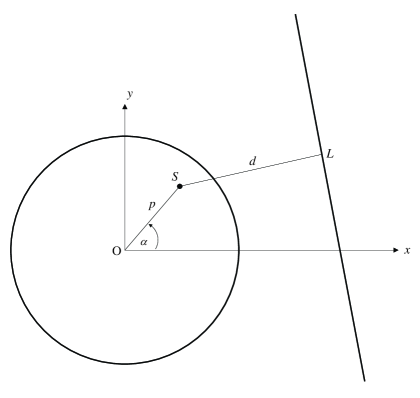
Figure 8: A schematic view of the source plane for a fold caustic crossing event, showing in projection (i.e. with the observer in the $z$ direction) the outer edge of the circumstellar envelope (of radius $r_{\rm max}$). The bold line represents a small portion of a closed caustic structure, approximated by a straight line. An element of the source, at $S$, with position defined by polar coordinates $p$ and $\alpha$, is shown; it lies at a projected perpendicular distance $d$ from the fold caustic. Note that the fold caustic will not, in general, be aligned with the direction of motion of the source (assumed here to be along the $x$-axis) so that the caustic may sweep across the source at an oblique angle.

4.2.1 Pure resonance lines

Figure 9: The lightcurve, equivalent widths and line profiles produced by a fold caustic crossing of a star with photospheric radius $R=0.003\,\theta_{E}$ surrounded by a circumstellar envelope exhibiting pure resonance line scattering. The three panels present results in the same manner as in Figures 6 and 7. All profiles were again calculated for an integrated optical depth of $T=3.0$ and assuming $x_{\rm max}=5$.

Figure 10: Same as for Figure 9, but now shown for a pure recombination line.

We next computed continuum lightcurves, line equivalent widths and line profiles for the case of a pure resonance line lensed by a fold caustic as the source exits the caustic structure. Illustrative results are shown in Figure 9 for a star with pseudo-photospheric radius $R=0.003\,\theta_{E}$ and assuming $x_{\rm max}=5$. The model line profile shown has $\rm T=3$.

The upper left hand panel of Figure 9 shows the change in apparent magnitude, computed from the ratio of lensed to unlensed continuum flux, as a function of time (again measured in units of $t_{E}$). Note that we consider here only the effect of the excess magnification due to the extra images produced by the caustic structure; in other words we are assuming that the term $A_{0}$ in equation (42) is a constant during the caustic crossing, and can therefore be subtracted from the total magnification, leaving only the differential effect of the two extra images. Hence the magnitude change due to the extra images alone drops to zero after the photosphere has fully exited the fold caustic.

The lower left hand panel of Figure 9 shows the time evolution of the line equivalent width, calculated as before. We see that the equivalent width first rises gently as the fold caustic begins to cross the circumstellar envelope and differentially magnifies the line emission from the wind relative to the continuum. The increase in equivalent width is at first modest, however, because the absorption components of the line profile also receive some differential magnification at this stage. Indeed once the fold caustic begins to cross the star, the dominant effect of the differential magnification is to enhance the attenuated continuum flux from the pseudo-photosphere – thus resulting in a sharp dip in the equivalent width which reaches its minimum value at epoch (b). Thereafter the equivalent width begins to rise dramatically. This is because an increasing fraction of the pseudo-photosphere now lies outside the caustic structure, so that the relative effect of the lens on the circumstellar material which still lies inside is significantly enhanced. This effect reaches its peak shortly after epoch (c), by which time the photosphere lies entirely outside the caustic but a portion of the circumstellar envelope still lies inside, and thus continues to be differentially magnified due to the existence of the two extra images. As the fold caustic then sweeps across the rest of the envelope, the equivalent width drops sharply again, although at epoch (d) the equivalent width is still somewhat larger than at epoch (c) – as is evident in the profiles shown in the right hand panel.

4.2.2 Pure recombination lines

Finally we computed continuum lightcurves, line equivalent widths and line profiles for the case of a pure recombination line lensed by a fold caustic as the source exits the caustic structure. Illustrative results are shown in Figure 10 for eaxctly the same lens and source parameters as in Figure 9.

The upper left panel of Figure 10 is again identical to that of Figure 9. From the lower left panel we see that the time evolution of the line equivalent width shows qualitatively similar behaviour to that of Figure 9, although again the magnitude of the change in equivalent width is significantly larger for a recombination line than for a resonance line – as we also found for a point lens event. The stronger signature of lensing is also clearly seen in the right hand panel of Figure 10, where the lensed line profiles at epochs (a) to (d) show significantly greater enhancement of the emission near line centre than the enhanced emission at the corresponding epochs of Figure 9, or in Figure 7 for a recombination line lensed by a point mass lens.

Thus we can see collectively from these illustrative figures that the time evolution of the equivalent width as the lensing event proceeds can be an effective diagnostic of the radial extent of the circumstellar envelope. The equivalent width variations will also be sensitive to the integrated optical depth of the line; as we saw in Figures 3 and 4 increasing $\rm T$ resulted in a stronger line. Therefore, by studying the time evolution of equivalent width for a number of different lines, microlensing can in principle be a powerful probe of the run of optical depth as a function of radius in the circumstellar envelope.

5 Discussion

In this paper we have modelled the effects of microlensing for variations of line profiles formed in circumstellar envelopes. Although the microlensing is quantitatively accurate, the underlying wind model includes a number of simplifying assumptions: the flow is assumed to be spherically symmetric; resonance and recombination lines are both treated, but without detailed consideration of ionization or temperature gradients in the flow; the wind velocity law is treated as a linear function of radius; the envelope is truncated at some maximum radius; Sobolev theory is employed for the line formation. The intention of our modeling has been to assess relative effects from the line variations for an illustrative model, one that has generic application to stellar winds, but that would nonetheless require modification when applied to any particular case.

At this juncture it is useful to comment on the diverse kinds of winds observed across the Hertzsprung-Russell Diagram (hereafter, “HRD”). Referring to the introductory stellar winds book by Lamers & Cassinelli (1999), most stellar winds fall into two primary classes, these being radiatively driven or pressure driven. Of the former, line-driven winds are the primary consideration for hot OB stars (e.g., see review by Kudritzki & Puls 2000) as basically described by the CAK theory of Castor, Abbott, & Klein (1975). Line-driving is also relevant for the central stars of planetary nebulae that show Wolf-Rayet-like spectra (Tylenda, Acker, & Stenholm 1993). The Main Sequence hot stars exhibit absorption line spectra from their photospheres; however, strong and weak P Cygni lines are abundant at UV wavelengths (Howarth & Prinja 1989; Snow et al. 1994). In the evolved hot stars, recombination lines appear at IR wavelengths (e.g., Lenorzer et al. 2002). Also, a substantial fraction (around a quarter, although the value is uncertain) of B stars are classified as emission-line or “Be” stars (Porter & Rivinius 2003). These have circumstellar disks that produce copious recombination lines in the IR, but more interestingly show H$\alpha$ in emission, which would be relevant for ground-based follow-up monitoring programs. Unfortunately, hot stars are relatively rare and so are extremely unlikely to be background sources for microlensing events.

Working toward cooler temperatures in the HRD, the winds from Main Sequence stars A–M are not well-studied, in part because their mass loss is so much weaker than early-type stars. The yellow hypergiants have more substantial winds, but these stars are extremely rare (de Jager 1998). A subclass of the A stars are strongly magnetic – the Ap and Am stars. These represent $\sim 10$% of the A-star class (MacGregor 2005), and are stars with surface magnetic fields in the multi-kilo-Gauss range, often modelled as oblique magnetic rotators in which the magnetic field is predominantly dipolar (Stibbs 1950). The wind diagnostics, particularly the portion trapped by the global dipolar magnetic field loops, are likely to be found in the X-ray band, as the trapped wind streams from opposite hemispheres are forced by the magnetic field into supersonic collisions to generate shock-heated gas (e.g., Babel & Montmerle 1997; Townsend & Owocki 2005). Again, these types of stars are not often expected in finite-source microlensing events. The solar-type star observed in the extended source event reported in Abe et al. (2003) presumably has a solar-like stellar wind, with a feeble mass-loss rate of order $10^{-14}\,M_{\odot}$ yr^-1. Consequently, wind spectral features accessible to ground-based follow-up would be essentially non-existent for such a source; instead, coronal diagnostics would be found in the UV and X-ray bands. Although one might expect to see effects in Ca ii H and K that are sensitive to chromospheric emission, our model line profiles are not appropriate for the quasi-static chromosphere.

The most likely class of stars to be found as sources in microlensing transit events, either by a single or a binary lens, are the red giant stars, a consequence of their being reasonably common and fairly large in size. Red giant winds have modest mass-loss rates of order $10^{-10}$ or $10^{-8}M_{\odot}$ yr^-1; however, even these estimates are not certain because the origin of their winds is not well-understood. The absence of X-ray emission for K and M giants (Linsky & Haisch 1979) indicates that their winds are not Parker-like, although they do show chromospheric features. The strong Mg ii h and k lines and Fe ii lines can be used to probe cool star winds; however, these lines are found in the UV which is not amenable to ground-based follow-up. It may be that a combination of molecular opacity and some dust formation drives the winds of red giants (Jorgensen & Johnson 1992), and perhaps certain molecular lines could be used as wind diagnostics.

Red supergiants (RSG) and asymptotic giant branch (AGB) stars have more interesting wind features that could be studied in microlensing transits. These are stars with high mass-loss rates of order $10^{-5}M_{\odot}$ yr^-1. They are radiatively driven, but unlike the early-type stars that are line driven, these stars are continuum driven because of substantial dust formation in their dense and cool winds. Simmons et al. (2002) have explored the possibility that scattering polarization could be used to probe their winds, but of course this is a continuous opacity. Similar to the red giants, UV lines can be used to probe the wind flow. Some of RSG and AGB stars also show maser emission lines at radio frequencies (Elitzur 1992; Habing 1996; Lewis 1998). These are thought to form primarily in shells. Consequently, the model lines presented in this paper are less likely to be relevant, although the considerations of Ignace & Hendry (1999) might be more appropriate, if suitably modified for the emissivity function of the maser. Once again, stars of the RSG and AGB classes are fairly rare.

There are two other classes of sources for which our line profile models are more relevant. One is the active galactic nuclei (AGN) that produce strong wind flows (Arav et al. 1995; Proga, Stone, & Kallman 2000). The (rest frame) UV spectra of quasars show some quite strong P Cygni profiles, such as in C iv, suggesting wind speeds in excess of 10,000 km s^-1. The flows are likely line-driven similar to early-type stars. Already, some authors have modelled the characteristic emission line profile effects that would be observed for different source models during microlensing events (Popović, Mediavilla, & Muñoz 2001; Abajas et al. 2002), ranging from Keplerian disks to relativistic disks to simple shells and jets. The microlensing under consideration was by a single deflector; however, our spherically symmetric wind models are not directly applicable to these cases that mostly involve non-spherical geometries. Some have claimed the detection of microlensing effects relevant to probing the AGN accretion disk (e.g., Chae et al. 2001), although none have reported effects pertinent to a wind component. We will not discuss this class further, and have mentioned it only because the general consideration of emission profile variations during microlensing events involving wind flows has been considered in the context of AGN.

The second class of objects are supernovae (and the likely related gamma-ray bursters). The explosions of stars spew gaseous ejecta into space. There is a phase in which the ejecta follows homologous expansion, not because the flow is accelerating, but because the ejecta is moving outward with a distribution of speeds. Still, the flow can be modeled as a wind, and the spectra at different phases shows numerous wind-features, ranging from strong P Cygni lines, to recombination lines, to forbidden lines (Filippenko 1997). Because supernovae (SNe) are so intrinsically luminous at early times, they can be seen to large distances, and so the probability of lensing increases owing to the considerable cosmological path lengths involved.

Recently Dalal et al. (2003) have discussed the impact of weak lensing due to large scale structure on the use of SNe as standard candles. Other authors have considered microlensing as a tool for studying the ejecta of SNe and even gamma-ray bursts (GRBs). For example, Schneider & Wagoner (1987) considered polarimetric variations of pseudo-photospheres produced in SNe during a microlensing event. Bagherpour, Branch, & Kantowski (2005) modelled the impact of microlensing on P Cygni line profiles in the spectra of Type Ia SNe. Gaudi, Granot, & Loeb (2001) have invoked microlensing to explain a brightening event in the lightcurve of GRB-000301C. However, thus far a more comprehensice study that systematically explores the effects of microlensing on emission line features formed in SN and GRB ejecta remains to be made; our illustrative results presented here are a further step in that direction.

With respect to SNe, there are several points of caution to be made when applying the results of this paper. First, our models assume a steady-state source. Of course, the luminosities, ejecta optical depth, and photospheric radii evolve with time in real SNe. Our results are applicable to SNe if the lensing event is relatively fast compared to photometric and structural changes of the ejecta. Under what conditions will this be true? Suppose we take the duration of the lensing event to be one week. If the fastest ejecta shell moves at $10^{4}$ km s^-1, then the extent of the ejecta shell would be at least $r_{\rm max}\approx 40$ AU at early phases of the explosion in which homologous expansion is applicable. Moreover, the evolution must be such that the lens moves across the ejecta shell (in projection) before the dimensions of the photosphere change significantly. This means the proper motion of the lens should greatly exceed that of the photospheric expansion. Given the $10^{4}$ km s^-1 ejecta speed as a maximum, and assuming a transverse velocity of $10^{2}$ km s^-1 for the lensing mass, we require that $D_{\rm SN}\gg D_{\rm L}$. Consequently, if the lens were located at kpc distances (e.g., in the halo, the bulge, or the Large Magellanic Cloud), then the SN should be located at Mpc distances (e.g. at the distance of the Virgo cluster).

As a consistency check, we compare the angular size of the SN ejecta $\theta_{\rm SN}$ to $\theta_{\rm E}$, as given by

$$\frac{\theta_{\rm SN}}{\theta_{\rm E}}=\frac{r_{\rm max}/D_{\rm SN}}{\sqrt{\left(R_{\rm L}/D_{\rm L}\right)\,\left(1-D_{\rm L}/D_{\rm SN}\right)}}.$$ (43)

If we assume the lensing object to be typical of MACHOs of about $0.5M_{\odot}$, then the Schwarzschild radius of the lens $R_{\rm L}$ will be of order 1 km. If we further assume $r_{\rm max}\approx 40$ AU, and $D_{\rm SN}\gg D_{\rm L}$, then

$$\frac{\theta_{\rm SN}}{\theta_{\rm E}}\approx\frac{100\;{\rm kpc}}{D_{\rm SN}},$$ (44)

where $D_{\rm L}=10$ kpc was assumed. Thus, SNe at distances of several to dozens of Mpc would have $\theta_{\rm SN}/\theta_{\rm E}\approx 0.01-0.1$ at early phases in the SN when homologous expansion remains valid. These happen to be values typical of our model simulations.

A further assumption of our models has been the common “core-halo” treatment, in which we can approximate the photosphere as a “hard” spherical boundary, and the wind features are all formed exterior to this boundary. Recent radiative transfer simulation of Type II SNe by Dessart & Hillier (2005) show this not to be true. Instead, the radiative transfer in SNe ejecta is more akin to that of Wolf-Rayet stars, for which the continuum forms in the wind flow.

The purpose of our models has not been to represent rigorously any particular type of stellar wind or class of stars, but to illustrate the generic effects that could be observed with intensive follow-up programs for source transit microlensing events. In so doing, models for two common types of lines have been considered – resonance P Cygni lines and recombination emission lines, for both point lensing and caustic crossing events from binary lensing. Whether the source is a hot star or a cool star, whether the lines are in the X-ray band or the radio band, the general properties of the line variations in terms of lead/lag times relative to the photosphere, of equivalent width variations, and changes in line profile shape are qualitatively all to be expected. We imposed the homologous expansion as a representative flow velocity law. Observationally, the velocity law is something that would preferably be determined from the line variations as the microlensing event evolved. With the photospheric crossing time determined from the photometric variations, the variations of the line equivalent width and profile changes with time could be converted to radius, calibrated by the photospheric radius, to deduce flow velocity and opacity variations.

- (1) Abajas C., Mediavilla E., Munoz J. A., Popovic L. C., Oscoz A. 2002, ApJ 576,
- (2) be F., Bennett D. P., Lgerkvist C. I, et al. A&A, 411, 493
- (3) Afonso C., Alard C., Albert J.N. et al. 2000, ApJ, 532, 340
- (4) Albrow M., Beaulieu J. P., Birch P. et al. 1998, ApJ, 509, 687
- (5) Albrow M., Beaulieu J. P., Caldwell J. A. R. et al. 1999, ApJ, 522, 1022
- (6) Albrow M., Beaulieu J. P., Caldwell J. A. R. et al. 2000, ApJ, 534, 894
- (7) Albrow M., An J., Beaulieu J. P. et al. 2001a, ApJ, 549, 759
- (8) Albrow M., An J., Beaulieu J. P. et al. 2001b, ApJ, 550, 173
- (9) Alcock C., Allen W. H., Allsman R. A. et al. 1997, ApJ 491, 436
- (10) Arav N., Korista K. T., Barlow T. A., Begelman M. C. 1995, Nat. 376, 576
- (11) Babel, J., Montmerle, T. 1997, A&A 323, 121
- (12) Bagherpour, H., Kantowski, R., Branch, D., Richardson, D. 2004, astro-ph/0411622
- (13) Bagherpour, H., Branch, D., Kantowski, R. 2005, astro-ph/0503460
- (14) Bryce H. M., Ignace, R., Hendry, M. A. 2003, A&A, 401, 339
- (15) Castor, J. I., Abbott, D. C., Klein, R. I. 1975, ApJ 195, 157
- (16) Chae, K.-H., Turnshek, D. A., Schulte-Ladbeck, R. E., Rao, S. M., Lupie, O. L. 2001, ApJ 561, 653
- (17) Coleman, I. J., Simmons, J. F. L., Newsam, A. M., Bjorkman, J. E. 1997. In: Ferlet, R. et al. (eds.) Variable Stars and the Astrophysical Returns of the Microlensing Surveys (Editions Frontieres) p. 147
- (18) Coleman, I. J. 1998, Ph.D. Thesis, University of Glasgow
- (19) Dalal, N., Holz, D. E., Chen, X., Frieman, J. A. 2003, ApJ, 585, 11
- (20) de Jager, C. 1998, A&ARv 8 145
- (21) Dessart, L., Hillier, D. J. 2005, A&A 437, 667
- (22) Elitzur, M. 1992, ARAA 30, 75
- (23) Fields, D. L., Albrow, M. D., An, J. et al. 2003, ApJ, 596, 1305
- (24) Filippenko, A. V. 1997, ARAA 35, 309
- (25) Gaudi, B. S., Granot, J., Loeb, A. 2001, ApJ 561, 178
- (26) Gould A. 2001, PASP 113, 903
- (27) Habing, H. J. 1996, A&ARv, 7, 97
- (28) Hauschildt, P. H., Allard F., Baron E. 1999, ApJ, 525, 871
- (29) Heyrovský, D., Sasselov, D., Loeb, A. 2000, ApJ, 543, 406
- (30) Howarth, I. D., Prinja, R. K. 1989, ApJS 69, 527
- (31) Ignace, R., Hendry, M. A. 1999, A&A, 341, 201
- (32) Jorgensen U. G., Johnson H. R. 1992, A&A 265, 168
- (33) Kudritzki, R.-P., Puls, J. 2000, ARAA 38, 613
- (34) Kurucz, R. L. 1994, Atlas CDROMs (Email: kurucz@cfa.harvard.edu)
- (35) Lamers, H., Cassinelli, J. 1999, Introduction to Stellar Winds (Cambridge University Pres)
- (36) Lenorzer, A., Vandenbussche, Morris, P. 2002, A&A 384, 473
- (37) Lewis, B. M. 1998, ApJ 508, 831
- (38) Linksy, J. L, Haisch, B. M. 1979, ApJ 229, L27
- (39) MacGregor, K. B. 2005, in The Nature and Evolution of Disks Around Hot Stars, Ignace and Gayley (eds.), ASP Conf. Ser. 337, 28
- (40) Mihalas D. 1978, Stellar Atmospheres, (Freeman: New York)
- (41) Paczyński B. 1986, ApJ, 304, 1
- (42) Popović, L. C., Mediavilla, E. G., Muñoz, J. A. 2001, A&A, 378, 295
- (43) Porter, J. M., Rivinius, Th. 2003, PASP 115, 1153
- (44) Proga, D., Stone, J. M., Kallman, T. R. 2000, ApJ 543, 686
- (45) Schneider, P., Wagoner, R. V. 1987, ApJ 314, 154
- (46) Schneider, P., Ehlers, J., Falco, E. E. 1992, Gravitational Lenses (Springer-Verlag)
- (47) Simmons, J. F. L., Bjorkman, J. E., Ignace, R., Coleman, I. J. 2002, MNRAS 336, 501
- (48) Snow, T. P., Lamers, J. G. L. M., Lindholm, D. M., Odell, A. P. 1994, ApJS 95, 163
- (49) Stibbs, D. W. N. 1950, MNRAS 110, 395
- (50) Townsend, R. H. D., Owocki, S. P. 2005, MNRAS 357, 251
- (51) Tylenda, R., Acker, A., Stenholm, B. 1993, A&AS 102, 595