Spitzer Mid-infrared Spectroscopy of Ices toward Extincted Background Stars

Abstract

A powerful way to observe directly the solid state inventory of dense molecular clouds is by infrared spectroscopy of background stars. We present Spitzer/IRS 5-20 µm spectra of ices toward stars behind the Serpens and Taurus molecular clouds, probing visual extinctions of 10-34 mag. These data provide the first complete inventory of solid-state material in dense clouds before star formation begins. The spectra show prominent 6.0 and 6.85 µm bands. In contrast to some young stellar objects (YSOs), most ($\sim$75%) of the 6.0 µm band is explained by the bending mode of pure H₂O ice. In realistic mixtures this number increases to 85%, because the peak strength of the H₂O bending mode is very sensitive to the molecular environment. The strength of the 6.85 µm band is comparable to what is observed toward YSOs. Thus, the production of the carrier of this band does not depend on the energetic input of a nearby source. The spectra show large abundances of CO and CO₂ (20-40% with respect to H₂O ice). Compared to YSOs, the band profile of the 15 µm CO₂ bending mode lacks the signatures of crystallization, confirming the cold, pristine nature of these lines of sight. After the dominant species are removed, there are residuals that suggest the presence of minor species such as HCOOH and possibly NH₃. Clearly, models of star formation should begin with dust models already coated with a fairly complex mixture of ices.

1. Introduction

Infrared absorption studies of protostars embedded in dense clouds have shown that dust grains along these lines of sight have icy mantles (e.g., Willner et al. 1982, Tielens et al. 1984, Allamandola et al. 1992, Whittet et al. 1996, Boogert et al. 2004). Heating by the protostar and energetic photons can affect the ice composition by sublimation and by triggering chemical reactions (e.g., Gerakines et al. 1996, Ehrenfreund & Charnley 2000, Schutte & Khanna 2003). Knowledge of the ice composition in quiescent dense clouds is required in determining the amount of processing ices undergo during star formation. This ‘baseline’ can be obtained by observations of field stars lying behind molecular clouds. These observations also help constrain models of chemical evolution during the star forming process (e.g., Lee et al. 2004).

The 3 µm absorption band of H₂O ice was observed toward stars behind the Serpens (Eiroa & Hodapp 1989) and Taurus dark clouds (Whittet et al. 1988, Smith et al. 1993, Murakawa et al. 2000). These studies indicate that H₂O ice is formed deep in the clouds, at visual extinctions $A_{\rm V}>3$ magnitudes (the ice formation threshold). Solid CO was observed toward background stars as well (e.g., Whittet et al. 1985, Chiar et al. 1994, 1995). Its formation threshold is significantly larger ($A_{\rm V}$=6-15 mag) due to the lower sublimation temperature of solid CO.

Studies of ices toward background stars have been limited to bands below 5 µm because of telluric absorption and the fact that stellar fluxes drop rapidly with increasing wavelength. Observations of background stars have become increasingly feasible with the Infrared Space Observatory (ISO) mission and, in particular, with the launch of the Spitzer Space Telescope (Werner et al. 2004). With ISO, solid CO₂ at 4.25 µm was observed toward two Taurus background stars (Whittet et al. 1998; Nummelin et al.  2001), indicating that radiation from nearby protostars is not required to form this species. Recent observations with Spitzer detected the CO₂ bending mode at 15 µm toward background stars (Bergin et al. 2005). Here we present observations of ices toward three background stars over the full 5-20 µm range taken with the Infrared Spectrograph (IRS; Houck et al. 2004) aboard Spitzer. We assess the complete ice inventory in quiescent clouds and compare it to observations toward protostars.

2. Observations and Reduction

The background stars discussed here include a source behind the Serpens dark cloud, CK 2, and two sources behind the Taurus dark cloud, Elias 13 and Elias 16. The observations are part of the “c2d” legacy program (Evans et al.  2003). All sources were observed with the short wavelength, low resolution module (SL; $\lambda=$ 5-14 µm; $R\equiv\lambda/\Delta\lambda=$ 64-128), with on-source integration times of 28 sec per spectral order. CK 2 and Elias 13 were also observed with the short wavelength, high resolution module (SH; $\lambda=$ 10-20 µm; $R=600$), with integration times of 240 sec and 60 sec per spectral order, respectively. Spectra of Elias 13, Elias 16 and CK 2 were part of AOR# 0005636864, 0005637632, and 0011828224. The SH spectrum of Elias 16 has been published by Bergin et al. (2005) and was part of AOR# 0003868160. The data were reduced using the Spitzer Science Center (SSC) pipeline version S11.0.2 (S12 for SH in Elias 16) to produce the 2-dimensional Basic Calibrated Data. Subsequently, customized source extractions were performed, including the subtraction of extended background emission. The spectra were then defringed with sine-wave fitting routines (Lahuis & Boogert 2003).

Figure 1 shows the Spitzer spectra of the observed background stars, complemented by near-infrared (NIR) broad band photometry (2MASS). In addition, for CK 2, Spitzer IRAC (S. T. Megeath, priv. comm.) and ground-based L^′ band photometry (Churchwell & Koornneef 1986) are included and for Elias 16 the 2-5 µm ISO spectrum is shown (Whittet et al. 1998).

In order to put the data on an optical depth scale and analyze the ice and dust features, each spectrum is normalized to the spectrum of an extincted late-type giant taken from the ISO database (Sloan et al. 2003). A blackbody is used at wavelengths below 2.5 µm to fit the NIR photometry. The extinction law used for Serpens is of the form $A_{\lambda}\sim\lambda^{-1.9}$ (Kaas et al. 2004), whereas that for Taurus has a shallower power law, $A_{\lambda}\sim\lambda^{-1.7}$ (Whittet et al. 1988). Indebetouw et al. (2005) find a shallower slope on the extinction curve beyond 6 µm. This flattening is partly due to the silicate and ice features which we account for separately and the powerlaw is a good approximation to the extinction at longer wavelengths. $A_{\rm V}$ is taken to be 9.1 $\times$ $A_{\rm K}$ (Rieke & Lebofsky 1985). Spectral types K4 III, G9 III, and K3 III were adopted for CK 2, Elias 13 and Elias 16, respectively. These values are within the range of types given in Chiar et al. (1994) for CK 2 and close to the K2 III type assigned by Smith et al. (1993) for Elias 13 and 16. While the selected spectral types give the best fit (in removing the photospheric CO and SiO bands at 5 and 8 µm), they are uncertain by a few subclasses resulting in an abundance error of 20% on the strong features, especially since the available ISO database has limited coverage.

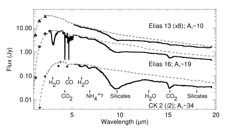
Figure 1.— The spectra of Elias 13, Elias 16 and CK 2 with the extincted photospheres (dashed lines) used for normalization. Near-infrared complementary data are shown in triangles, diamonds and plus signs, respectively. The spectra are scaled along the flux axis with the numbers given in brackets.

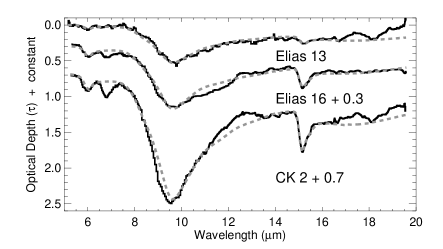
Figure 2.— Background star spectra on optical depth scale (black). A fit (dashed grey) of small spherical silicate grains is shown to which are added laboratory spectra of H₂O and CO₂ (at 15 µm) at intensities corresponding to the column densities mentioned in Table 1.

3. Results

3.1. CO₂ and H₂O Ices

The CO₂ 15 $\mu$m feature is very strong toward CK 2 and Elias 16, and weakly detected toward Elias 13. The abundance of CO₂ relative to H₂O is 33% toward CK 2, higher than the $\sim$20% abundance seen toward the Taurus sources. The derived CO₂ column densities toward Elias 13 and Elias 16 agree within errors with those obtained from the 4.25 µm feature (Nummelin et al. 2001; Table 1). The bottom of the 15 µm CO₂ feature appears single peaked toward all sources (Fig. 3) and does not show double dips due to crystallization as some protostars do (Gerakines et al. 1999, Boogert et al. 2004). The profile of this band toward Elias 16 is fitted in Bergin et al. (2005) with the sum of the polar (H₂O:CO₂=7:1) and the apolar (CO:CO₂=4:1) mixtures. The polar, H₂O-rich mixture accounts for 85% of the CO₂ column density. However, the H₂O column density assumed in this fit overestimates the observed value by 30%. We require that both the observed H₂O and CO₂ column densities, as well as the CO₂ band profile are matched. We use a combination of two polar mixtures H₂O:CO₂=1:1 and H₂O:CO₂=10:1 (with the ratios of the two mixtures: 2:1 for CK 2, 1.3:1 for Elias 16 and 1:0 for Elias 13) and the apolar mixture CO:N₂:CO₂=100:50:20, all at low temperature (Ehrenfreund et al. 1997). Satisfactory fits are obtained for polar fractions of 78% in CK 2, 84% in Elias 16, and 87% in Elias 13, comparable to the fractions found by Bergin et al (2005) despite the different mixtures used.

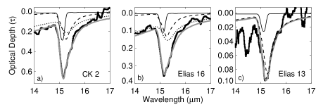
Figure 3.— CO₂ feature for a) CK 2, b) Elias 16 and c) Elias 13 compared to laboratory spectra composed of H₂O:CO₂=10:1 (dot) and 1:1 (dash) at 10 K and CO:N₂:CO₂=100:50:20 (thin solid) at 30 K. The grey line shows the best composite fit. Note that the vertical offset is due to the H₂O libration mode.

Using the H₂O ice column densities from the 3 µm band (Table 1) and laboratory spectra of pure H₂O ice (Hudgins et al. 1993), the H₂O bending mode contributes to 77% and 69% of the observed 6.0 µm absorption feature for Elias 16 and CK 2 (Fig. 2). However, the peak position, width, and strength of this band change significantly when H₂O is diluted. For example, compared to pure H₂O, the mixture H₂O:CO₂=1:1 shifts the peak to longer wavelengths by $\sim$0.1 µm, and increases the peak by a factor of 2.4, but the extensive long wavelength wing remains unchanged. Using mixtures that fit the 15 µm CO₂ band (Fig. 3), $\sim$85-100% of the 6.0 µm feature can be explained by H₂O (Fig. 4). The strong libration mode of H₂O explains much of the excess absorption in the 12-13 µm region, but due to severe blending with the silicate absorption feature, residuals in that spectral region are hard to interpret (§3.3). A model of astronomical silicates (Weingartner & Draine 2001) is used to fit the 10 and 20 µm features for all sources (Fig. 2), but this silicate model may not be unique.

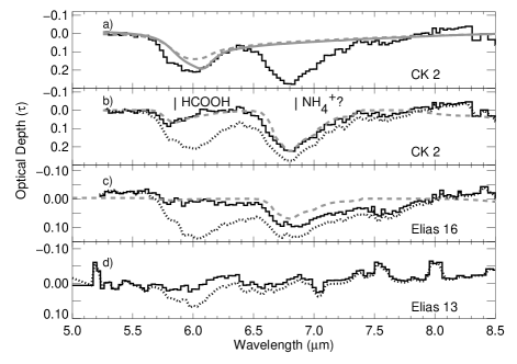
Figure 4.— a)The spectrum of CK 2 after removing silicate absorption is shown in black. The dash grey line is the pure H₂O-ice contribution to the 6.0 µm feature while the solid grey is the H₂O:CO₂ mixture. b-d) The dotted lines show the spectra after removing the silicate contribution. The solid lines show the spectra after removing silicate and H₂O contributions. b) For CK 2, the dash grey line shows a fit to HCOOH (5.85 and 8.2 µm), NH${}_{4}^{+}$ (6.85 µm) and NH₃ (6 µm). c) For Elias 16, the dash grey line shows a fit to NH${}_{4}^{+}$ and NH₃. d) For Elias 13, no remaining features are found.

3.2. The 6.85 µm Band and Other Ices

A strong feature at 6.85 µm is detected toward CK 2 and Elias 16 but not toward Elias 13. This is the first detection of this band toward background stars. It is commonly observed toward protostars (Keane et al. 2001) and often attributed to the NH${}_{4}^{+}$ ion (see Schutte & Khanna 2003; §4). Regardless of the identification, the profile may be a powerful tracer of the thermal history of the ices. Figure 5 shows the decomposition of the 6.85 µm feature into the short and long wavelength components used by Keane et al. (2001) to characterize this band. The phenomenological separation is meant to represent NH${}_{4}^{+}$ bands at different temperatures. The ratio of the peak optical depths of the two components (short/long) is 2 for Elias 16 and 1.2 for CK 2. If instead the equivalent widths are compared, the ratios are 1.6 and 0.9, respectively. In either case, the profiles resemble those of the protostars with the coldest sight-lines (e.g., NGC 7538 IRS9). Its equivalent width is used to calculate the column density for NH${}_{4}^{+}$ (Table 1) using the band strength from Schutte & Khanna (2003).

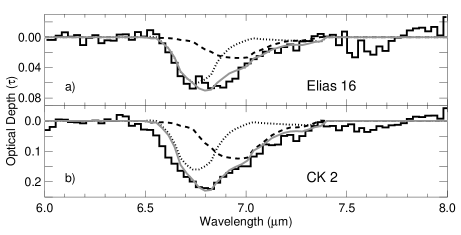
Figure 5.— The decomposition of the 6.85 µm feature into short (dot) and long wavelength (dash) components (Keane et al. 2001) for a) Elias 16 and b) CK 2. The solid grey line indicates the sum of the short and long wavelength components. The solid black line represents the spectrum after subtraction of silicate and H₂O contributions.

3.3. Other Ices and Hydrogen Column Densities

H₂O ice accounts for up to $85\%$ of the 6.0 µm absorption band for CK 2 (Fig. 4; §3.1). Some excess absorption remains, in particular on the short wavelength side. This is observed towards protostars as well, and attributed in part to absorption by HCOOH (Schutte et al. 1999, Keane et al. 2001). The 5.85 µm band is the strongest HCOOH band in our observed wavelength range, that at 8.2 µm is slightly weaker. For CK 2, the laboratory spectrum of pure solid HCOOH fits the 5.85 µm feature with a discrepancy at 8.2 µm, which may indicate over-correction of the photospheric SiO band (§2). Table 1 shows upper limits and tentative detections of weak features in the 7–13 µm spectral region.

Table 1Column Densities and Abundances

Species	Unit	CK 2	EL 13	EL 16	HH461	B51
CO	%H2O	362,	94	264	20	43
		573
CO2	%H2O	33	$\leq$15,	185,226,	32	37
			225	197,24
HCOOH	%H2O	1.9	…	…	$<$8.7	9.3
CH3OH	%H2O	$<$2.1	$<$0.8	$<$2.3	7.0	$<2.3$
NH3	%H2O	$\leq$8	$<$6	$\leq$8	17	$<$9.1
NH${}_{4}^{+}$	%H2O	10.8	…	5.5	9.6	$<$12.7
CH4	%H2O	$<$3	…	$<$3	4	…
OCN-	%H2O	…	…	$<$2.38	$\leq$0.7	$<$0.5
H2O	1018 cm-2	3.59	1.010	2.510	8.4	2.6
H	1022 cm-2	6.4	1.9	3.6	5.0	3.2

References. — 1. HH46 IRS and B5 IRS1 from Boogert et al. 2004, and in preparation; 2. Chiar et al. 1994; 3. Pontoppidan, et al. 2003; 4. Chiar et al. 1995; 5. Whittet et al. 1998, 6. Nummelin et al. 2001; 7. Bergin et al. 2005, 8. Whittet et al. 2001; 9. Eiroa & Hodapp 1989; 10. Whittet et al. 1988, Smith et al. 1993

The uncertainty in the shape of the silicate feature is large in some places (e.g., 20$\%$ at 10–13 µm) and hard to quantify in others. For ice abundance determinations, the hydrogen column density is usually calculated from the relation $N_{\rm H}\approx 1.87\times 10^{21}\times A_{\rm V}$ cm^-2 for $R_{\rm V}=3.1$ (Draine 2003). As outlined in §2, by fitting ISO template spectra, extinctions $A_{\rm V}$ of 34^m, 19^m, and 10^m are derived for CK 2, Elias 16, and Elias 13 respectively. The observed peak optical depth of the silicate band and the relation $A_{\rm V}$/$\tau_{9.7}$$=18.5\pm 2$ (Draine 2003) give similar values for $A_{\rm V}$. The $N_{\rm H}$ values listed in Table 1 are calculated using the $A_{\rm V}$ values derived from the photospheric fits.

4. Conclusions

Our Spitzer spectra of background stars show clear detections of absorption features at 6.0 and 6.85 µm that had previously only been seen toward YSOs, imposing new constraints on the origin of the 6.85 µm band. The strength of the 6.85 µm band, scaled to H₂O, is similar to that seen toward YSOs, as is the factor of 2 variation between sight-lines (Table 1; Schutte & Khanna 2003). In one scenario, the 6.85 µm band is explained by NH${}_{4}^{+}$ produced by acid-base reactions in ice mixtures containing NH₃ and HNCO. In laboratory experiments such reactions occur at temperatures as low as 10 K with conversion factors between 15% and 100% depending on ice mixtures and temperature (van Broekhuizen et al. 2004). The strength of the 6.85 µm band is a factor of 2 larger toward CK 2 compared to Taurus. This sight line probes a very cold region, as evidenced by the very high abundance of the volatile apolar CO ice ($T_{\rm subl}\sim$20 K) as well as the smooth profile of the 15 µm CO₂ band. In contrast, the line of sight of the YSO HH46 IRS shows evidence for the ices to have undergone thermal processing (Boogert et al. 2004), but the 6.85 µm band is not unusually deep (Table 1). Thus, if the 6.85 µm band is due to NH${}_{4}^{+}$, variables other than temperature, such as the initial HNCO and NH₃ abundances, must play roles in determining its strength. We stress that the identification of the 6.85 µm band with NH${}_{4}^{+}$ is tentative and more evidence, including correlation with the bands of counter ions such as OCN^- (van Broekhuizen et al. 2005) or HCOO^- is required.

Most ($\sim$75%) of the 6.0 µm band toward background stars is explained by pure H₂O ice, comparable to the percentage toward most massive YSOs (Keane et al. 2001). While H₂O mixed with CO₂ can explain the remaining absorption in the Taurus sources, the residual toward CK 2 has a peak absorption wavelength consistent with HCOOH (Fig. 4). Its abundance would be a few % of H₂O, comparable to that seen in several high-mass YSOs (Keane et al. 2001) but not as high as seen in some low-mass YSOs (Boogert et al., in preparation).

Dust grains have accumulated rather complex icy mantles in opaque regions of molecular clouds before star formation begins, a point which must be included in models of star formation. Also, the effect of freeze-out on the thermal balance has been studied by Goldsmith (2001). For the two stars with extinctions above 15 mag, the abundances relative to H₂O ice are within the range seen toward embedded objects. From the abundances in Table 1, the percentages of nitrogen, oxygen and carbon locked in ices for Elias 16 and CK 2 are 35-37% N, 28-30% O and $\sim$12% C. Further work on larger samples of background stars will elucidate the dependence of the ice composition on cloud conditions and history. Such surveys are now possible with Spitzer/IRS for sources as weak as 10 mJy (9.5 mag) at 8 µm and $A_{\rm V}$ of up to 50 mag.

References

- (1)
- (2) Allamandola, L. J., Sandford, S. A., Tielens, A. G. G. M., & Herbst, T. M. 1992, ApJ, 399, 134
- (3) Bergin, E. A., Melnick, G. J., Gerakines, P. A., Neufeld, D. A., & Whittet, D. C. B. 2005, ApJ, 627, L33
- (4) Boogert, A. C. A., et al. 2004, ApJS, 154, 359
- (5) Chiar, J. E., Adamson, A. J., Kerr, T. H., & Whittet, D. C. B. 1994, ApJ, 426, 240
- (6) —–. 1995, ApJ, 455, 234
- (7) Churchwell, E. & Koornneef, J. 1986, ApJ, 300, 729
- (8) Draine, B. T. 2003, ARA&A, 41, 241
- (9) Ehrenfreund, P., Boogert, A. C. A., Gerakines, P. A., Tielens, A. G. G. M., & van Dishoeck, E. F., 1997, A&A, 238, 649
- (10) Ehrenfreund, P. & Charnley, S. B. 2000, ARA&A, 38, 427
- (11) Eiroa, C. & Hodapp, K.-W. 1989, A&A, 210, 345
- (12) Evans, N. J., II et al. 2003, PASP, 115, 965
- (13) Gerakines, P. A., Schutte, W. A., & Ehrenfreund, P. 1996, A&A, 312, 289
- (14) Gerakines, P. A., et al. 1999, ApJ, 522, 357
- (15) Houck, J. R. et al. 2004, ApJS, 154, 18
- (16) Hudgins, D. M., Sandford, S. A., Allamandola, L. J., & Tielens, A. G. G. M. 1993, ApJS, 86, 713
- (17) Kaas, A. A. et al. 2004, A&A, 421, 623
- (18) Keane, J. V., Tielens, A. G. G. M., Boogert, A. C. A., Schutte, W. A., & Whittet, D. C. B. 2001, A&A, 376, 254
- (19) Lahuis, F., & Boogert, A. 2003, in Chemistry as a Diagnostic of Star Formation, eds. C.L. Curry & M. Fich (NRC Press, Ottawa), p. 335
- (20) Lee, J.-E., Bergin, E. A., & Evans, N. J.,II. 2004, ApJ, 617, 360
- (21) Murakawa, K., Tamura, M., & Nagata, T. 2000, ApJS, 128, 603
- (22) Nummelin, A., Whittet, D. C. B., Gibb, E. L., Gerakines, P. A., & Chiar, J. E. 2001, ApJ, 558, 185
- (23) Pontoppidan, K. M., et al. 2003, A&A, 408, 981
- (24) Rieke, G. H., & Lebofsky, M. J. 1985, ApJ, 288, 618R
- (25) Schutte, W. A., et al. 1999, A&A, 343, 966
- (26) Schutte, W. A. & Khanna, R. K. 2003, A&A, 398, 1049
- (27) Sloan, G. C., Kraemer, K. E., Price, S. D., & Shipman, R. F. 2003, ApJS, 147, 379
- (28) Smith, R. G., Sellgren, K., & Brooke, T. Y. 1993, MNRAS, 263, 749
- (29) Tielens, A. G. G. M., Allamandola, L. J., Bregman, J., Goebel, J., Witteborn, F. C., & Dhendecourt, L. B. 1984, ApJ, 287, 697
- (30) van Broekhuizen, F. A., Keane, J. V., & Schutte, W. A. 2004, A&A, 414, 425
- (31) van Broekhuizen, F. A., Pontoppidan, K. M., Fraser, H. J., & van Dishoeck, E. F. 2005, A&A, 441, 249
- (32) Weingartner, J. C. & Draine, B. T. 2001, ApJ, 548, 296
- (33) Werner, M. W. et al. 2004, ApJS, 154, 1
- (34) Whittet, D. C. B., McFadzean, A. D., & Longmore, A. J. 1985, MNRAS, 216, 45P
- (35) Whittet, D. C. B., Bode, M. F., Longmore, A. J., Adamson, A. J., McFadzean, A. D., Aitken, D. K., & Roche, P. F. 1988, MNRAS, 233, 321
- (36) Whittet, D. C. B., et al. 1996, A&A, 315, L357
- (37) Whittet, D. C. B., et al. 1998, ApJ, 498, L159
- (38) Whittet, D. C. B., Pendleton, Y. J., Gibb, E. L., Boogert, A. C. A., Chiar, J. E., & Nummelin, A. 2001, ApJ, 550, 793
- (39) Willner, S. P., et al. 1982, ApJ, 253, 174
- (40)