XMM-Newton observes ClJ0152.7$-$1357: A massive galaxy cluster forming at merger crossroads at $z=0.83$.

Abstract

We present an analysis of a $50\mbox{$\mathrm{~{}ks}$}$ XMM-Newton observation of the merging galaxy cluster ClJ0152.7$-$1357 at $z=0.83$. In addition to the two main subclusters and an infalling group detected in an earlier Chandra observation of the system, XMM-Newton detects another group of galaxies possibly associated with the cluster. This group may be connected to the northern subcluster by a filament of cool ($1.4^{+0.3}_{-0.1}\mbox{$\mathrm{~{}keV}$}$) X-ray emitting gas, and lies outside the estimated virial radius of the northern subcluster. The X-ray morphology agrees well with the projected galaxy distribution in new K-band imaging data presented herein. We use detailed spectral and imaging analysis of the X-ray data to probe the dynamics of the system and find evidence that another subcluster or group has recently passed through the northern subcluster. ClJ0152.7$-$1357 is an extremely dynamically active system with mergers at different stages occurring along two perpendicular merger axes.

1. Introduction

Clusters of galaxies are believed to form hierarchically via the collapse and merger of smaller structures. Massive clusters form most recently in this scenario, and indeed, X-ray substructure which is indicative of merger and formation activity is found to be more prevalent in clusters at high redshifts (Jeltema et al., 2005). Observations of merging systems at high redshift thus enable the study of the process of cluster formation. X-ray observations provide a useful tool in this study, enabling measurements of the properties of the dominant baryonic component of clusters and detecting merger-related features like shocks (e.g. Markevitch et al., 2002) and cold fronts (e.g. Markevitch et al., 2000; Vikhlinin et al., 2001) in the X-ray emitting gas.

In cosmological simulations, the most massive clusters form at the intersections of the filaments of structure (e.g. Jenkins et al., 1998). While filamentary structures are observed in the large scale distributions of galaxies (e.g. Colless et al., 2001), they are rarely observed in X-rays (Scharf et al., 2000; Durret et al., 2003; Ebeling et al., 2004) because of their low gas densities. Cluster mergers have also been detected in X-rays at the meeting points of apparent filaments, for example in Abell 85 (Durret et al., 2003, 2005), Abell 521 (Arnaud et al., 2000; Ferrari et al., 2005) and Coma (e.g. Neumann et al., 2003). ClJ0152.7$-$1357 is an example of a massive, high-redshift merging system located in a network of large-scale structures (Kodama et al., 2005), and so presents a valuable opportunity to observe the hierarchical formation of structure.

ClJ0152.7$-$1357 was discovered in the Wide Angle ROSAT Pointed Survey (WARPS: Scharf et al., 1997; Ebeling et al., 2000). It was also discovered independently in the RDCS (Rosati et al., 1998) and SHARC (Romer et al., 2000) surveys and was spectroscopically confirmed at a redshift of $z=0.83$ Ebeling et al. (2000); Della Ceca et al. (2000). Analysis of the discovery ROSAT data found the system to be highly luminous with considerable X-ray substructure consisting of two probable subclusters (Ebeling et al., 2000). The cluster has also been the subject of BeppoSAX observations (Della Ceca et al., 2000) and Sunyaev-Zel’dovich effect imaging (Joy et al., 2001). A Chandra ACIS-I observation enabled the two subclusters to be fully resolved and detected a galaxy group near the cluster to the east (Maughan et al., 2003). The Chandra data were used to measure the temperatures of the two subclusters separately for the first time, confirming that they are both hot ($\sim 5.5\mbox{$\mathrm{~{}keV}$}$) and massive.

More recently, ClJ0152.7$-$1357 has been the subject of detailed studies at optical wavelengths. Demarco et al. (2005) confirmed 102 cluster member galaxies with VLT spectroscopy and found that the eastern group was at the same redshift as the cluster. Girardi et al. (2005) used this redshift information to perform a detailed dynamical analysis of the system. The distribution of galaxies around this system was probed out to scales of $\sim 5\mbox{$\mathrm{~{}Mpc}$}$ using photometric redshifts obtained with Subaru by Kodama et al. (2005). In addition, this remarkable system has been the subject of weak lensing analyses, both ground based (Huo et al., 2004) and with the HST (Jee et al., 2005). Broadly speaking, the distributions of X-ray emitting gas, cluster galaxies, and dark matter are found to be similar.

In this paper we present the results of an analysis of an XMM-Newton observation of ClJ0152.7$-$1357 along with new K-band imaging. The large collecting area of XMM-Newton enables the most detailed X-ray study yet of this system. A $\Lambda$CDM cosmology of $H_{0}=70\mathrm{\mbox{$\mathrm{~{}km}$}\mathrm{\mbox{$\mathrm{~{}s}$}^{-1}}\mathrm{\mbox{$\mathrm{~{}Mpc}$}^{-1}}\,}$, and $\Omega_{\mathrm{M}}=0.3$ ($\Omega_{\Lambda}=0.7$) is adopted throughout, and all errors are quoted at the $68\%$ level. At the cluster redshift of $0.83$, $1\mathrm{{}^{\prime}}\hskip-1.00006pt\mathrm{{}^{\prime}}$ corresponds to $7.6\mbox{$\mathrm{~{}kpc}$}$ in our chosen cosmology.

2. Data Reduction

2.1. XMM-Newton data

ClJ0152.7$-$1357 was observed by XMM-Newton for $50\mbox{$\mathrm{~{}ks}$}$ on 2002 December 24 (ObsID 0109540101). The data were reduced and analysed using the XMM-Newton Science Analysis Software (SAS) version 6.1 with the latest calibration products available in April 2005. A binned image of the field observed by XMM-Newton EPIC is shown in Fig. 1. The target cluster and the galaxy NGC 0720 (detected by chance at the edge of the field) are labelled.

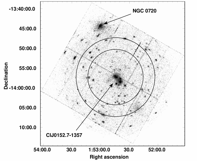
Figure 1.— Binned X-ray image of the field of view. Labels indicate the target cluster and the galaxy NGC 0720 which was observed by chance at the edge of the field. The annulus indicates the region used for the measurement of the background emission.

Periods of background flaring were detected and removed by applying an iterative sigma-clipping algorithm to lightcurves of the data from the PN and two MOS detectors. This was first done for lightcurves of the whole field in the $10-15\mbox{$\mathrm{~{}keV}$}$ band with time bins of $50\mbox{$\mathrm{~{}s}$}$ and a $3\sigma$ threshold. The observation was virtually unaffected by background flares, and after cleaning $48\mbox{$\mathrm{~{}ks}$}$ ($53\mbox{$\mathrm{~{}ks}$}$) of useful PN (MOS) data remained. The results of this cleaning were checked by applying the same procedure to lightcurves of source-free regions in the $2-15\mbox{$\mathrm{~{}keV}$}$ band with $200\mbox{$\mathrm{~{}s}$}$ bins and a $2\sigma$ threshold. The results of this stricter broad-band cleaning were completely consistent with those of the high-energy band cleaning, and the good time intervals defined in the $10-15\mbox{$\mathrm{~{}keV}$}$ band were applied to the data used in all further analysis.

In the spectral analysis of extended sources, the precise modeling or subtraction of the background emission is crucial, particularly in regions of low surface brightness. The compact angular size of ClJ0152.7$-$1357 relative to the XMM-Newton field of view means that the background emission local to the source can be used obtain background spectra. The annulus used for measuring the local background emission is marked in Fig. 1, and has inner and outer radii of $7\arcmin$ ($3.2\mbox{$\mathrm{~{}Mpc}$}$) and $10\arcmin$ ($4.6\mbox{$\mathrm{~{}Mpc}$}$) respectively. Note that all sources within this region were excluded in our analysis, but these are not marked on the Figure in order to preserve clarity. As this background region is further from the optical axis than the source, the emission in the region will be vignetted (the mean effective area in the background region is $\sim 60\%$ of that at the optical axis). The effects of vignetting were accounted for in the imaging analysis with the use of exposure maps, and in all spectral analysis by using the SAS task evigweight along with on-axis effective area files.

All spectral analysis was also performed using the blank sky data sets of Read & Ponman (2003) with the “double subtraction” method of Arnaud et al. (2002). In this method background spectra are extracted from the same detector regions as the source spectra, but from the blank sky datasets. A background region of the source dataset (in this case the annulus marked in Fig. 1) is used to derive a residual spectrum to account for any differences (predominantly at low energies due to different levels of soft Galactic background) between the source and blank sky fields. The final background spectrum consists of the blank sky spectrum plus the residual spectrum (scaled for any differences in extraction area). The exposure times of the blank sky observations were normalised so that the count rates of events detected outside the telescopes’ field of view in the target and blank sky datasets matched. Fig. 2 shows the PN background spectra extracted from the background annulus region in the source and blank sky datasets. The spectra agree well in the fluorescent lines at $1.5\mbox{$\mathrm{~{}keV}$}$ and $8\mbox{$\mathrm{~{}keV}$}$ but the normalisation of the continuum in the blank sky spectrum is too high. This indicates that the level of the particle-induced background (which is responsible for the out of field of view counts and dominates the fluorescent line flux) is higher in the source dataset than the blank sky observations. Alternatively if the blank sky spectra were normalised to match the continuum level, the normalisation of the fluorescent lines would be incorrect. Both of these differences would be compensated for to some extent by the residual spectrum that is added to the blank sky spectrum.

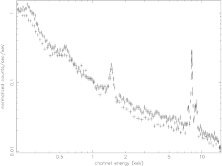
Figure 2.— XMM-Newton PN background spectra obtained from the background annulus region in the source field (black) and blank sky dataset (grey). The blank sky spectrum was normalised by the flux of events detected outside the field of view.

Despite these differences, almost all of the temperatures measured with the double subtraction blank sky background method were consistent with those measured by adopting a local background alone (see §5.3 for the exception). This is most likely due to the correcting effect of the residual spectrum, and the fact that the slope of the blank sky background spectrum continuum is the same as the local background. It should be noted, however, that the statistical uncertainties on the spectral properties measured in the low surface brightness regions of this data where the background contribution is important are large. Thus the effects of the systematic differences between the local and blank sky backgrounds cannot be sensitively tested. With those caveats, we conclude that a simple local background, extracted from the source dataset, and vignetting-corrected with evigweight is the more reliable method for this particular dataset, and this is used for all spectral results presented here.

2.2. Near-infrared data

K band observations of ClJ0152.7-1357 were made with IRIS2 (the near-infrared imager and spectrograph) on the 3.9m Anglo-Australian Telescope, Siding Spring, Australia, on 2003 September 5, and 2004 January 10. The conditions on both occasions were clear, and the seeing was $\approx 1.7\mathrm{{}^{\prime}}\hskip-1.00006pt\mathrm{{}^{\prime}}$ and $1.3\mathrm{{}^{\prime}}\hskip-1.00006pt\mathrm{{}^{\prime}}$ in September and January respectively.

The images were dark-subtracted, flat-fielded and mosaiced using standard techniques with the iraf software package. Flatfields were created by median combining the jittered object frames. The total exposure time of all observations was 205 minutes.

3. Imaging analysis

A spectrally-weighted exposure map was produced for each EPIC camera, to account for the energy dependence of the telescope vignetting function. Exposure maps were produced in narrow energy bands, within which the vignetting function varied little, and these were weighted according to the relative contribution of each band to an assumed spectral model. An absorbed MeKaL model with $kT=5.5\mbox{$\mathrm{~{}keV}$}$, appropriate for ClJ0152-7$-$1357 (Maughan et al., 2003, and §4), was used. All of the X-ray imaging analysis was performed in the $0.3-5\mbox{$\mathrm{~{}keV}$}$ energy band.

A mosaiced image of the emission detected by the three cameras was then produced, and exposure corrected. This image was adaptively smoothed to show real features detected at the $3\sigma$ level with the asmooth algorithm of Ebeling et al. (2005), and logarithmically spaced contours of this smoothed emission are shown overlaid on a NIR image in Fig. 3. All of the sources in Fig. 3 except for those labelled are point sources, with the possible exception of the north eastern most source at $\alpha[2000.0]=01^{\rm h}52^{\rm m}45.64^{\rm s}$ $\delta[2000.0]=-13^{\circ}55\mathrm{{}^{\prime}}29.0\mathrm{{}^{\prime}}\hskip-1.00006pt\mathrm{{}^{\prime}}$. Based on the redshifts measured by Demarco et al. (2005), the brightest X-ray source near the subclusters ($\alpha[2000.0]=01^{\rm h}52^{\rm m}43.62^{\rm s}$ $\delta[2000.0]=-13^{\circ}59\mathrm{{}^{\prime}}1.0\mathrm{{}^{\prime}}\hskip-1.00006pt\mathrm{{}^{\prime}}$) appears associated with a cluster member galaxy, and the point source at $\alpha[2000.0]=01^{\rm h}52^{\rm m}34.62^{\rm s}$ $\delta[2000.0]=-13^{\circ}59\mathrm{{}^{\prime}}30.2\mathrm{{}^{\prime}}\hskip-1.00006pt\mathrm{{}^{\prime}}$. Within the size of the XMM-Newton point spread function (PSF), there are two cluster member galaxies and one foreground galaxy coincident with the point source at $\alpha[2000.0]=01^{\rm h}52^{\rm m}39.75^{\rm s}$ $\delta[2000.0]=-13^{\circ}57\mathrm{{}^{\prime}}42.8\mathrm{{}^{\prime}}\hskip-1.00006pt\mathrm{{}^{\prime}}$.

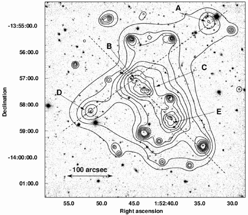
Figure 3.— Adaptively smoothed contours of the X-ray emission detected from ClJ0152-7$-$1357 with XMM-Newton are overlaid on the K band IRIS2 image. The dashed lines indicate the two apparent merger axes of the system and the labels are described in the text and summarised in Table 1.

The complex morphology of the extended emission in ClJ0152.7$-$1357 is immediately apparent in Fig. 3. The north and south subclusters (labelled C and E in Fig. 3) and the group to the east (D) were all detected in the Chandra observation of this system (Maughan et al., 2003). In addition, XMM-Newton also detects an envelope of low surface brightness emission surrounding the subclusters and eastern group, which extends in a apparent filament to a second group (A) to the north-west. The redshift of this group is unknown. However, while the associated galaxies were not included in the VLT observations of Demarco et al. (2005), the group’s position appears to coincide with a clump of galaxies of the same photometric redshifts as ClJ0152.7$-$1357 in Kodama et al. (2005). We address the question of whether this north-west group is associated with the main cluster in more detail later. The morphology of the system suggests intersecting north-east to south-west and south-east to north-west merger axes, which are indicated in Fig. 3.

Fig. 3 also shows that the X-ray emission from the north subcluster is extended in the northern direction, with a possible second X-ray peak (labelled B). This extension is in the direction of an overdensity of galaxies slightly further north, which also appears as a peak in the weak lensing mass map of Jee et al. (2005).

For convenience, the labelled regions in Fig. 3 are summarised in Table 1.

Table 1Summary of the structures labelled in Fig. 3

Region	$\alpha[2000.0]$	$\delta[2000.0]$	Description
A	$01^{\rm h}52^{\rm m}34.18^{\rm s}$	$-13^{\circ}54\mathrm{{}^{\prime}}42.3\mathrm{{}^{\prime}}\hskip-1.00006pt\mathrm{{}^{\prime}}$	North west group of unknown redshift
B	$01^{\rm h}52^{\rm m}45.15^{\rm s}$	$-13^{\circ}57\mathrm{{}^{\prime}}02.4\mathrm{{}^{\prime}}\hskip-1.00006pt\mathrm{{}^{\prime}}$	Northern extension of north subcluster
C	$01^{\rm h}52^{\rm m}43.76^{\rm s}$	$-13^{\circ}57\mathrm{{}^{\prime}}24.4\mathrm{{}^{\prime}}\hskip-1.00006pt\mathrm{{}^{\prime}}$	North subcluster
D	$01^{\rm h}52^{\rm m}51.99^{\rm s}$	$-13^{\circ}58\mathrm{{}^{\prime}}13.2\mathrm{{}^{\prime}}\hskip-1.00006pt\mathrm{{}^{\prime}}$	Galaxy group at cluster redshift
E	$01^{\rm h}52^{\rm m}39.83^{\rm s}$	$-13^{\circ}58\mathrm{{}^{\prime}}26.7\mathrm{{}^{\prime}}\hskip-1.00006pt\mathrm{{}^{\prime}}$	Southern subcluster

The distribution of NIR light in ClJ0152.7$-$1357 was also investigated with the K band imaging data. The NIR luminosity of a galaxy is well correlated with its dynamical mass (Gavazzi et al., 1996), making the K band an excellent choice with which to trace out the distribution of galaxies within the cluster. The image was divided into a grid of 1000$\times$1000 bins, and the number of galaxies detected at a significance $\geq 3\sigma$ in each bin was counted. Objects which were brighter than the brightest known members were excluded. Due to the poor seeing, the galaxy density may be underestimated in the highest density regions. However, all of the known members from Demarco et al. (2005) were included by manually deblending some of the galaxies. An image of this map was created and adaptively smoothed at the 90% level. Contours of galaxy number density are shown overlaid on a K band image and a smoothed X-ray image in Fig. 4. There is a clear similarity in the galaxy and X-ray distribution; both the subclusters and groups are apparent. An overdensity of galaxies to the north of the X-ray emission in region B is also clear.

The comparison of Figs. 3 and 4 shows a clear offset between the peak of the galaxy light and X-ray emission in the southern subcluster. This was first noticed in the Chandra observation of ClJ0152.7$-$1357 by Maughan et al. (2003) who suggested that the offset was due to the collisionless galaxies (and presumably dark matter) moving ahead of the X-ray gas which is slowed by ram pressure due to the merger. Jee et al. (2005) found similar offsets between the mass peaks of both subclusters in their weak lensing analysis and the X-ray centroids, which is consistent with this explanation. We note, however that the X-ray peak of the northern subcluster is coincident with that of the galaxy distribution, but the northern extension of that subcluster (likely due to another merger) leads to an apparent offset between the X-ray centroid and galaxy distribution.

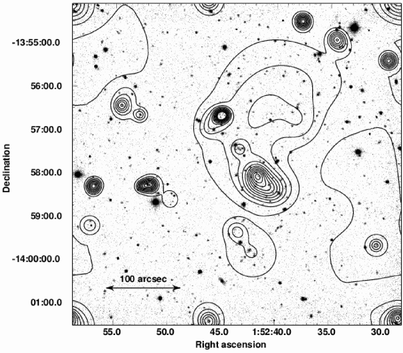
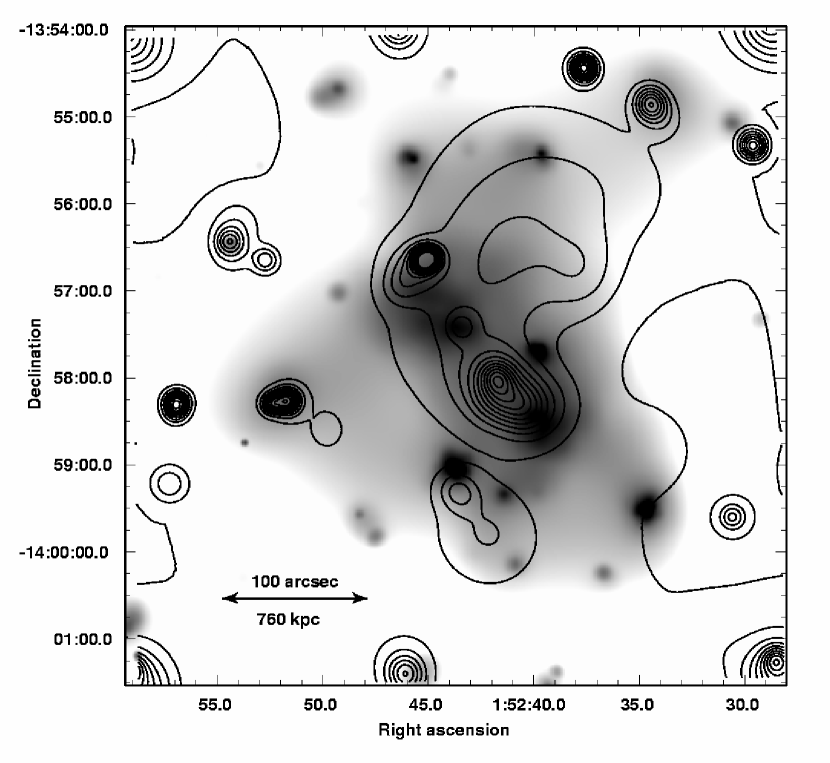
Figure 4.— Left: Contours of constant galaxy number density derived from the AAT K-band images are overlaid on the same NIR image. The contours have been adaptively smoothed at 90% significance. Right: The same contours are overlaid on the smoothed X-ray image from which the X-ray contours in Fig. 3 were taken.

3.1. X-ray surface brightness modeling.

The two-dimensional (2D) X-ray surface brightness distribution in ClJ0152-7$-$1357 was modeled in Sherpa with an elliptical $\beta-$model for each of the two subclusters and two groups, and a flat and a vignetted background (see Maughan et al., 2004, for a more detailed description of the method). Due to the low surface brightness of the two groups, their model ellipticities were fixed at zero and their core radii were fixed at $100\mbox{$\mathrm{~{}kpc}$}$. This core radius is appropriate for the temperatures of these groups as measured in §4 (Sanderson et al., 2003). The models were fit simultaneously to binned images for each EPIC camera after being convolved with the appropriate PSF and exposure map. All model parameters except for the amplitudes were tied between the different detectors. The background levels were determined from a fit to a local source free region and fixed.

The data residuals from the best-fitting models for each camera were combined and smoothed with a Gaussian of $\sigma=12\mathrm{{}^{\prime}}\hskip-1.00006pt\mathrm{{}^{\prime}}$ (3 image pixels). The resulting image is shown in Fig. 5. Point sources were excluded both during the fitting process and from these residuals. There are several regions of excess emission above the model visible in Fig. 5. We note that some of these residual features occur near or across PN CCD gaps. However, they are also present in the residuals for the MOS detectors alone so are not due to exposure correction problems around the CCD gaps.

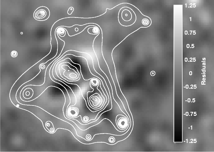
Figure 5.— Smoothed X-ray image of the residuals from the best-fitting model to the surface brightness distribution in ClJ0152-7$-$1357. Smoothed contours of X-ray surface brightness are overlaid.

In Fig. 6, contours of the positive surface brightness residuals are overlaid on the best-fitting surface brightness model, and on a NIR image. In this Figure, the surface brightness models for each detector have been summed, after convolution with the PSF and multiplication by the exposure map. The PN CCD gaps are thus visible in the surface brightness model. The same labels used in Fig. 3 are included to aid orientation. Positive residuals are associated with the subcluster cores (C and E), which may indicate the presence of dense cool cores, and also with region B. The region of excess emission at $\alpha[2000.0]=01^{\rm h}52^{\rm m}40.75^{\rm s}$ $\delta[2000.0]=-13^{\circ}56\mathrm{{}^{\prime}}33.1\mathrm{{}^{\prime}}\hskip-1.00006pt\mathrm{{}^{\prime}}$ to the west of region B is aligned with several faint galaxies, while that at $\alpha[2000.0]=01^{\rm h}52^{\rm m}42.71^{\rm s}$ $\delta[2000.0]=-13^{\circ}59\mathrm{{}^{\prime}}52.5\mathrm{{}^{\prime}}\hskip-1.00006pt\mathrm{{}^{\prime}}$ to the south east of the southern subcluster (E) coincides with several brighter galaxies. Both features appear to be associated with galaxies whose photometric redshifts are consistent with that of ClJ0152.7$-$1357 as measured by Kodama et al. (2005), and both appear in the contours of galaxy light in Fig. 4. While this is not statistically rigorous, it is likely that these regions of excess emission are linked to levels of substructure in the system which are not present in our simple surface brightness model. Similarly, the negative residuals to either side of the northern subcluster core in Fig. 5 are probably due to the inadequacy of a simple elliptical model to describe the subcluster.

There is excess emission between the the two main subclusters (C and E). This excess was also detected in the Chandra observation of ClJ0152.7$-$1357 by Maughan et al. (2003). A possible explanation for this feature proposed by Maughan et al. (2003) is a region of increased density due to the compression of the gas in the merger. However, the weak lensing mass reconstruction of this system by Jee et al. (2005) shows two mass peaks in this region, and there are also several cluster galaxies in this region (see Fig. 6). This suggests that the excess emission may be due to gas associated with mass clumps in this region, which may be additional subgroups or clusters in this complex system.

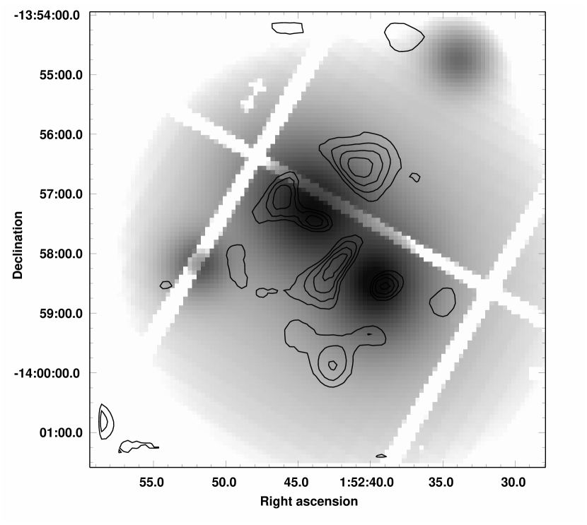
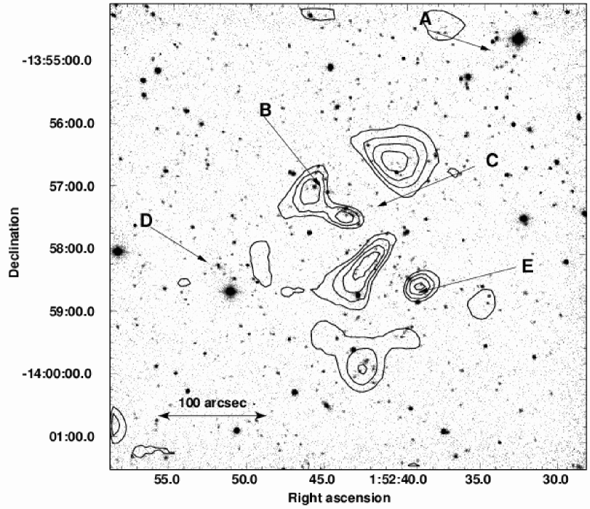
Figure 6.— Left: The best-fitting two-dimensional surface brightness model of ClJ0152.7$-$1357 with contours of the positive residuals overlaid. Right: The same contours are overlaid on an IRIS2 K band image, with the same labels used in Fig 3.

3.2. Projections of the X-ray surface brightness

An alternative way of visualising the data is to use projections of the surface brightness along different axes. In the case of ClJ0152.7$-$1357 the two merger axes are natural choices. A rectangular region aligned with each of the merger axis was defined. The X-ray counts in a combined PN and MOS $0.3-5\mbox{$\mathrm{~{}keV}$}$ image within this region were then projected onto its long axis. The same procedure was applied to combined PN and MOS image of the best-fit 2D model, after convolution with the PSF and exposure map. The data projection was adaptively binned to give fractional uncertainties of $\leq 10\%$ on each point.

Fig. 7 shows the projection along the south-east to north-west merger axis. For this axis, a region of width $75\mathrm{{}^{\prime}}\hskip-1.00006pt\mathrm{{}^{\prime}}$ centred on the two groups was used. Several features are labelled in Fig. 7, using the same labels as Fig. 3 and Table 1. The region between C and A corresponds to the apparent filament in Fig. 3. In this region, the model represents the simple superposition of the group and cluster emission and the data show no significant departure from this model. The filamentary appearance of the emission in this region could thus simply be due to the superposition of the cluster and group emission. However, given the difficulty of modeling the surface brightness distribution of this system, we cannot rule out the possibility of filamentary emission in this region. The point source visible in Fig. 3 halfway between B and A was excluded from the data and model in this projection.

Figure 7.— Projection of the surface brightness in a $75\mathrm{{}^{\prime}}\hskip-1.00006pt\mathrm{{}^{\prime}}$ wide region onto the south-east to north-west merger axis. The points show the projection of the imaging data and the solid line is the projection of the best-fit 2D model. The dashed line shows the locally estimated background level.

The projection of the north-east to south-west merger axis is shown in Fig. 8. A rectangular projection region of width $50\mathrm{{}^{\prime}}\hskip-1.00006pt\mathrm{{}^{\prime}}$ centred on the two subclusters was used. The substructure around region B in Fig. 3 is visible in this projection. Excess emission between the subclusters (C and E) is apparent, and a bright point source which was excluded from the 2D modeling, but not from the data in this projection is visible at the right end of Fig. 8. The disagreement between the model and data at the position of the chip gap at $230\mathrm{{}^{\prime}}\hskip-1.00006pt\mathrm{{}^{\prime}}$ is due to the imperfect exposure correction around the chip gap combined with the bright point source.

Figure 8.— Projection of the surface brightness in a $50\mathrm{{}^{\prime}}\hskip-1.00006pt\mathrm{{}^{\prime}}$ wide region onto the north-east to south-west axis. The points show the projection of the imaging data and the solid line is the projection of the best-fit 2D model. The dashed line shows the locally estimated background level.

4. Spectral Mapping

The high quality X-ray data enable spatially resolved temperature measurements of the gas in this merger. A method based on that described by O’Sullivan et al. (2005) was used to produce the temperature map. First, a “radius map” was produced, based on a binned X-ray image. The radius map recorded the radius of the circular region enclosing $>1000$ background-subtracted, point-source-excluded photons centered on each pixel in the binned image. A maximum radius of $60\mathrm{{}^{\prime}}\hskip-1.00006pt\mathrm{{}^{\prime}}$ was imposed, and pixels which failed to meet these criteria were excluded from the radius map. Spectra were then extracted for each pixel within the appropriate radius, and the three EPIC spectra were fit simultaneously with an absorbed MeKaL model. During the fitting process, the model parameters were tied except for the normalisations which were independent. The metal abundance was fixed at $0.3\mathrm{Z_{\odot}}$ using the abundance tables of Anders & Grevesse (1989), and the absorbing column was fixed at the Galactic value (Dickey & Lockman, 1990). All spectra were grouped to have at least 20 total counts per spectral bin, and were fit in the $0.3-7\mbox{$\mathrm{~{}keV}$}$ band using local background spectra extracted from the background annulus region (Fig. 1).

The resulting projected temperature map is shown in Fig. 9. It should be noted that the method used for producing the temperature map means that adjacent pixels are not independent. The radius map in Fig. 9 gives the extent of the spectral extraction region used at each pixel. Broadly speaking, the gas in the system has temperatures in the range $4-7\mbox{$\mathrm{~{}keV}$}$ but the spatial distribution of temperatures is not smooth. There are three apparently hotter regions in the temperature structure which are labelled in Fig. 9. The northern-most (kT1) is aligned with the residual emission at region B (see Figs. 5 and 6). The hotter regions at kT2 and kT3 are not associated with any surface brightness features. The mixing of spectra between adjacent pixels in this spectral mapping method can make such features appear more significant than they truly are, as they occur in several adjacent pixels. The temperatures and fit parameters of the hottest pixel in each of these regions are given in Table 2. While region kT1 is a local maximum in temperature, it is actually no hotter than the average temperature across the cluster of $5.5\mbox{$\mathrm{~{}keV}$}$. Regions kT2 and kT3, however, are hotter at the $\sim 2\sigma$ level. With the exception of pixels close to the boundaries of the temperature map, none of the measured temperatures are significantly cooler than $5.5\mbox{$\mathrm{~{}keV}$}$.

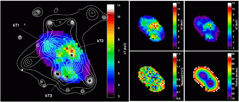
Figure 9.— Left: Projected temperature map of ClJ0152-7$-$1357 with contours of X-ray surface brightness overlaid. The spectral fit parameters of the labelled regions are given in Table 2. Right: The upper panels show the $1\sigma$ upper (left) and lower (right) limits on the temperature values. The lower panels show the reduced $\chi^{2}$ of the spectral fits and the radii used for spectral extraction.

A simple alternative method of producing a temperature map was also implemented. In this method geometrical regions were defined by hand using the surface brightness distribution and residuals as a guide. Spectra were extracted from these regions (with point sources excluded) and fit as above. Again, vignetting-corrected background spectra extracted from the background annulus region were used. The goal in following this method was to isolate some of the features in the system and obtain spectra that are free from the mixing effects of the previous method. We were also able to extract and fit spectra for regions which did not pass the binning algorithm’s criteria. Fig. 10 shows the resulting temperature map and the fit parameters of the numbered regions are given in Table 2. The table also gives the net source counts detected with each EPIC camera. We note that three of the regions (1, 2 and 7) have low net counts ($150-300$). This means that the grouping of the spectra to 20 total counts per bin and the use of the $\chi^{2}$ statistic may not be appropriate. In these cases, ungrouped versions of the spectra were also fit using the C statistic in XSPEC. In all cases, the temperatures and uncertainties were in good agreement with the ones quoted in Table 2.

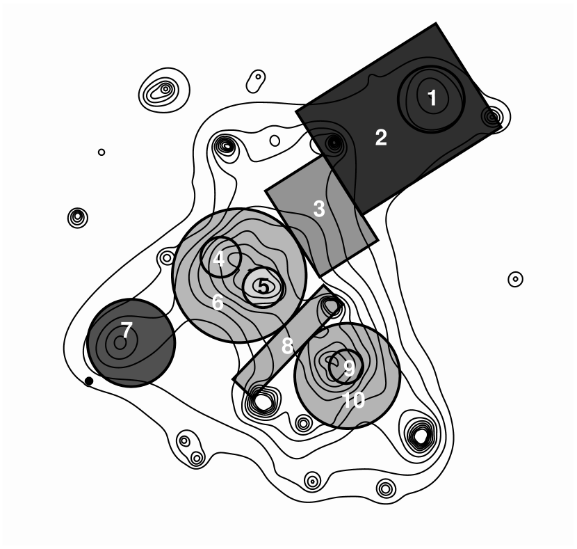
Figure 10.— Projected temperature map of ClJ0152-7$-$1357 with contours of X-ray surface brightness overlaid. Darker regions are cooler and lighter regions hotter. The fit parameters of the numbered regions are given in Table 2.

Table 2Values of the spectral fit parameters for the regions shown in Fig. 9 and Fig. 10

		Net Counts
Region	kT (keV)	PN	MOS1	MOS2	$\chi^{2}$	$\nu$
kT1	$5.9^{+0.9}_{-0.6}$	579	240	276	50.8	59
kT2	$10.3^{+3.0}_{-1.9}$	549	244	245	46.0	52
kT3	$7.3^{+1.4}_{-0.9}$	705	250	228	44.1	59
1	$1.5^{+0.2}_{-0.1}$	89	31	38	18.5	12
2	$1.4^{+0.3}_{-0.1}$	150	18	28	102.8	63
3	$4.4^{+1.0}_{-0.8}$	340	100	123	48.4	51
4	$5.6^{+1.1}_{-0.8}$	355	108	135	20.6	27
5	$6.4^{+0.8}_{-0.7}$	625	275	233	52.0	53
6	$5.4^{+0.4}_{-0.4}$	1425	620	682	157.7	159
7	$2.4^{+0.6}_{-0.4}$	179	76	61	26.5	31
8	$5.3^{+0.8}_{-0.7}$	506	161	170	42.6	44
9	$4.9^{+0.6}_{-0.5}$	499	188	212	45.4	38
10	$5.3^{+0.4}_{-0.4}$	1590	492	565	142	144

This method indicates that the two main subclusters and their surrounding regions have temperatures consistent with $5.5\mbox{$\mathrm{~{}keV}$}$. The eastern group (region 7) is significantly cooler at $2.4^{+0.6}_{-0.4}\mbox{$\mathrm{~{}keV}$}$, with a temperature, appropriate for a group or small cluster. The redshift of the north-west group (region 1) cannot be determined from the X-ray spectra, but under the assumption that it is at the cluster redshift it too has a low temperature consistent with a galaxy group. The emission in region 2, between group A and the northern subcluster also has a low temperature of $1.4^{+0.3}_{-0.1}\mbox{$\mathrm{~{}keV}$}$ assuming a redshift of $0.83$.

The regions associated with positive surface brightness residuals in the subcluster cores show no evidence for the cooler gas which would be expected if the excess emission were due to cool cores. However, the size of the regions are small ($\sim 30\mathrm{{}^{\prime}}\hskip-1.00006pt\mathrm{{}^{\prime}}$ diameter) so the blurring effect of the XMM-Newton PSF would make such emission more difficult to detect. The Chandra observation of this system, with its negligible PSF, also detects positive surface brightness residuals in the cluster cores, but the data quality is insufficient to extract spectra from those regions. The statistical uncertainties on the XMM-Newton temperatures along with the unaccounted for projection effects mean that the presence of cool cores in either subcluster cannot be ruled out.

Regions 3, 4 and 8 were also chosen based on the surface brightness residuals. These do not show departures from the subcluster temperatures. In particular, region 8 between the subclusters is not significantly hotter.

Finally, the global luminosity of the cluster was measured. Due to the complex morphology of the system, extrapolating luminosities measured from spectral fits to the individual components of the system out to a large radius may lead to inaccuracies. Instead, global spectra were extracted for each EPIC camera from within a radius of $1.4\mbox{$\mathrm{~{}Mpc}$}$ ($184\mathrm{{}^{\prime}}\hskip-1.00006pt\mathrm{{}^{\prime}}$, chosen to match the apertures used in Markevitch, 1998), after the exclusion of point sources. The resulting spectra were fit as before using the local background spectra, and the best fitting temperature was $3.7\pm 0.2\mbox{$\mathrm{~{}keV}$}$ ($\chi^{2}/\nu=588/558$). While the emission within this large aperture is clearly not isothermal, the spectra did not support the modelling of a second thermal component. The bolometric luminosity (rest frame $0.01-100\mbox{$\mathrm{~{}keV}$}$) within this aperture was measured to be $1.3\pm 0.2\times 10^{45}\mathrm{\mbox{$\mathrm{~{}erg}$}\mathrm{\mbox{$\mathrm{~{}s}$}^{-1}}}$. The uncertainties on the luminosity incorporate those on the best-fit temperature and normalisation of the spectral model.

5. Discussion

This deep XMM-Newton observation confirms the global temperatures measured by Chandra for the two main subclusters (Maughan et al., 2003), and supports the conclusion that ClJ0152.7$-$1357 is a massive merger. Maughan et al. (2003) included just the two main subclusters in their mass analysis, but the XMM-Newton temperatures of the two groups can be used to estimate their contribution to the total mass of the system. Using the high-redshift mass-temperature relation of Maughan et al. (2005) (based on a sample of relaxed and unrelaxed clusters including the two subclusters of ClJ0152.7$-$1357) we estimate that an object of $\sim 2\mbox{$\mathrm{~{}keV}$}$ will have a total virial mass of $\sim 1\times 10^{14}\mathrm{M_{\odot}}$. In the same way, the approximate temperature of the two subclusters ($5.5\mbox{$\mathrm{~{}keV}$}$) gives a mass of $\sim 5\times 10^{14}\mathrm{M_{\odot}}$ for each. We thus concluded that the mass of the system is $\sim 1\times 10^{15}\mathrm{M_{\odot}}$ (in line with Maughan et al., 2003) and that this is dominated by the two main subclusters.

In the following sections we discuss the important features of ClJ0152.7$-$1357 detected by XMM-Newton.

5.1. Substructure in the northern subcluster

The combination of the galaxy overdensity, weak-lensing mass peak and the X-ray substructure in the north of the northern subcluster (region B in Fig. 3) suggest the presence of a third subcluster or group in the NE-SW merger axis of the ClJ0152.7$-$1357. One plausible explanation for the configuration of the galaxy, gas, and dark matter distribution in this region is that the third subcluster has recently passed through the northern subcluster, traveling in a northerly direction. The dark matter and galaxies of the third subcluster were unaffected by the encounter due to their small (or non-existent) collisional cross sections. Its gas, meanwhile, was stripped from the potential, with the northern extension of the X-ray emission and possible second X-ray peak in that region being due to the surviving dense gas core of the third subcluster.

The mean redshift of the galaxies associated with this possible third subcluster is $0.838\pm 0.006$ (using the redshifts measured by Demarco et al., 2005); the same as that of the northern subcluster itself within the uncertainties. This suggests that any motion is in the plane of the sky.

5.2. The properties of group D

In their dynamical analysis of ClJ0152.7$-$1357, Girardi et al. (2005) find a velocity dispersion of $\sigma_{\mathrm{v}}\approx 700\mathrm{\mbox{$\mathrm{~{}km}$}\mathrm{\mbox{$\mathrm{~{}s}$}^{-1}}}$. The X-ray temperature of the group ($2.4^{+0.6}_{-0.4}\mbox{$\mathrm{~{}keV}$}$) is slightly low compared to the velocity dispersion (e.g. Xue & Wu, 2000), but it is consistent with the $\sigma_{\mathrm{v}}-T$ relation within the scatter. Using the MeKaL normalisation of the spectral fit in this region, and assuming that the group is spherical, the gas mass within a radius of $20\mathrm{{}^{\prime}}\hskip-1.00006pt\mathrm{{}^{\prime}}$ was estimated to be $6.0\pm 0.6\times 10^{11}\mathrm{M_{\odot}}$. This can be compared with the total mass within the same radius from the weak lensing data (Jee et al., 2005) to give a gas mass fraction of $f_{\mathrm{gas}}\approx 0.03$. At $z=0.83$ the radius of $20\mathrm{{}^{\prime}}\hskip-1.00006pt\mathrm{{}^{\prime}}$ corresponds to $150\mbox{$\mathrm{~{}kpc}$}$, so this gas fraction is measured only in the central region of group D. The gas fraction found is consistent with that measured in the central regions of local systems of a similar temperature (Sanderson et al., 2003).

5.3. Group A and the possible filament

Another interesting feature of the XMM-Newton data is the possibility that galaxy group A is falling into the cluster along a merger axis which runs through the northern subcluster (C) and group D. The K-band light distribution shows similar structure to the X-ray morphology in this region and the galaxies associated with the group are faint. However it is not known if the group is at the same redshift as the cluster.

The gas density in the region of emission between group A and the northern subcluster was estimated using the MeKaL normalisation from the spectral fit to region 2 (Fig. 10). In order to simplify the computation of the volume of region 2, the MeKaL normalisation was first scaled up to account for the area excluded in region 1. The volume of region 2 was then calculated assuming it is a cylinder with rotational symmetry about its long axis. With the simplifying assumption that the density is constant throughout that volume, the Hydrogen number density in this region is $4.0\pm 0.6\times 10^{-4}\mathrm{\mbox{$\mathrm{~{}cm}$}^{-3}}$. These results should be treated with some caution as the emission is very low surface brightness, and the issue of background subtraction is critical. In particular, while the results above were based on spectral fits with a local background, we were unable to obtain acceptable spectral fits with a blank sky background. However, the uncertainties in accounting for the differences in soft Galactic X-ray emission in the source and blank sky datasets are particularly important in the study of a region of low surface brightness, cool gas such as this. As discussed in §2, the use of a local background should to be the most reliable method in this instance.

It is interesting to compare this possible filament with the apparently isolated filament detected by Scharf et al. (2000) with ROSAT. The surface brightness in region 2 is $1.3\pm 0.4\times 10^{-15}\mathrm{\mbox{$\mathrm{~{}erg}$}\mathrm{\mbox{$\mathrm{~{}s}$}^{-1}}\mbox{$\mathrm{~{}cm^{-2}}$}}$ arcmin^-2. This is an order of magnitude brighter than the Scharf et al. (2000) filament. While that filament has no apparent connection to any massive clusters, it is likely that the gas densities would be higher in regions of filaments that are feeding onto a massive cluster of galaxies like that in ClJ0152.7$-$1357. However, as demonstrated in §3.2, the apparent filament may simply be due to the superposition of the emission from the group and cluster.

In order to estimate of the extent of the northern subcluster, a mass profile was derived assuming that the gas follows an isothermal $\beta$-profile in hydrostatic equilibrium with the cluster potential. While these are clearly gross simplifications for this complex system, they are sufficient for the purposes of estimating an approximate virial radius for the northern subcluster. The gas temperature of region 6 in Fig. 10 along with the $\beta$-profile parameters from the 2D surface brightness fitting ($r_{c}=40\pm 3\mathrm{{}^{\prime}}\hskip-1.00006pt\mathrm{{}^{\prime}}$, $\beta=0.86\pm 0.06$) were then used to estimate a virial radius of $R_{\mathrm{200}}\approx 1.3\mbox{$\mathrm{~{}Mpc}$}$. Here, we define the virial radius as the radius enclosing a mean density that is a factor of 200 times the critical density at $z=0.83$. Numerical simulations show that this overdensity radius approximately separates the virialised part of clusters from the infalling material surrounding them (Navarro et al., 1995). The estimated virial radius of the northern subcluster falls approximately halfway along region 2 in Fig. 10. Disregarding projection effects, the southern subcluster and group D all fall within the virial radius of the northern subcluster. If the group A is associated with the system, it is most likely at an earlier merger stage, lying outside the estimated virial radius.

6. conclusions

ClJ0152.7$-$1357 is a fascinating system, comprising two main subclusters in an apparently early stage of merging and possibly two infalling groups. There also is evidence for late stage merger activity in the northern subcluster. The formation of a massive cluster is occurring along two main merger axes which appear perpendicular in the plane of the sky. This unique system provides a dramatic example of cluster formation via mergers on different scales and at different stages, providing further compelling observational support for the hierarchical assembly model of cluster formation.

7. Acknowledgments

We thank Christine Jones for useful discussions of this work. BJM is supported by NASA through Chandra Postdoctoral Fellowship Award Number PF4-50034 issued by the Chandra X-ray Observatory Center, which is operated by the Smithsonian Astrophysical Observatory for and on behalf of NASA under contract NAS8-03060. SCE acknowledges PPARC support.

References

- Anders & Grevesse (1989) Anders, E. & Grevesse, N. 1989, Geochim. Cosmochim. Acta, 53, 197
- Arnaud et al. (2002) Arnaud, M., Majerowicz, S., Lumb, D., Neumann, D. M., Aghanim, N., Blanchard, A., Boer, M., Burke, D. J., Collins, C. A., Giard, M., Nevalainen, J., Nichol, R. C., Romer, A. K., & Sadat, R. 2002, A&A, 390, 27
- Arnaud et al. (2000) Arnaud, M., Maurogordato, S., Slezak, E., & Rho, J. 2000, A&A, 355, 461
- Colless et al. (2001) Colless, M., Dalton, G., Maddox, S., Sutherland, W., Norberg, P., Cole, S., Bland-Hawthorn, J., Bridges, T., Cannon, R., Collins, C., Couch, W., Cross, N., Deeley, K., De Propris, R., Driver, S. P., Efstathiou, G., Ellis, R. S., Frenk, C. S., Glazebrook, K., Jackson, C., Lahav, O., Lewis, I., Lumsden, S., Madgwick, D., Peacock, J. A., Peterson, B. A., Price, I., Seaborne, M., & Taylor, K. 2001, MNRAS, 328, 1039
- Della Ceca et al. (2000) Della Ceca, R., Scaramella, R., Gioia, I. M., Rosati, F., & Squires, G. 2000, A&A, 353, 498
- Demarco et al. (2005) Demarco, R., Rosati, P., Lidman, C., Homeier, N. L., Scannapieco, E., Benítez, N., Mainieri, V., Nonino, M., Girardi, M., Stanford, S. A., Tozzi, P., Borgani, S., Silk, J., Squires, G., & Broadhurst, T. J. 2005, A&A, 432, 381
- Dickey & Lockman (1990) Dickey, J. M. & Lockman, F. J. 1990, ARA&A, 28, 215
- Durret et al. (2005) Durret, F., Lima Neto, G. B., & Forman, W. 2005, A&A, 432, 809
- Durret et al. (2003) Durret, F., Lima Neto, G. B., Forman, W., & Churazov, E. 2003, A&A, 403, L29, lSS
- Ebeling et al. (2004) Ebeling, H., Barrett, E., & Donovan, D. 2004, ApJ, 609, L49
- Ebeling et al. (2000) Ebeling, H., Jones, L. R., Perlman, E., Scharf, C., Horner, D., Wegner, G., Malkan, M., Fairley, B., & Mullis, C. R. 2000, ApJ, 534, 133
- Ebeling et al. (2005) Ebeling, H., White, D., & Rangarajan, F. 2005, MNRAS
- Ferrari et al. (2005) Ferrari, C., Arnaud, M., Ettori, S., Maurogordato, S., & Rho, J. 2005, ArXiv Astrophysics e-prints
- Gavazzi et al. (1996) Gavazzi, G., Pierini, D., & Boselli, A. 1996, A&A, 312, 397
- Girardi et al. (2005) Girardi, M., Demarco, R., Rosati, P., & Borgani, S. 2005, A&A, 442, 29
- Huo et al. (2004) Huo, Z., Xue, S., Xu, H., Squires, G., & Rosati, P. 2004, AJ, 127, 1263
- Jee et al. (2005) Jee, M. J., White, R. L., Benítez, N., Ford, H. C., Blakeslee, J. P., Rosati, P., Demarco, R., & Illingworth, G. D. 2005, ApJ, 618, 46
- Jeltema et al. (2005) Jeltema, T. E., Canizares, C. R., Bautz, M. W., & Buote, D. A. 2005, ApJ, 624, 606
- Jenkins et al. (1998) Jenkins, A., Frenk, C. S., Pearce, F. R., Thomas, P. A., Colberg, J. M., White, S. D. M., Couchman, H. M. P., Peacock, J. A., Efstathiou, G., & Nelson, A. H. 1998, ApJ, 499, 20
- Joy et al. (2001) Joy, M., LaRoque, S., Grego, L., Carlstrom, J. E., Dawson, K., Ebeling, H., Holzapfel, W. L., Nagai, D., & Reese, E. D. 2001, ApJ, 551, L1
- Kodama et al. (2005) Kodama, T., Tanaka, M., Tamura, T., Yahagi, H., Nagashima, M., Tanaka, I., Arimoto, N., Futamase, T., Iye, M., Karasawa, Y., Kashikawa, N., Kawasaki, W., Kitayama, T., Matsuhara, H., Nakata, F., Ohashi, T., Ohta, K., Okamoto, T., Okamura, S., Shimasaku, K., Suto, Y., Tamura, N., Umetsu, K., & Yamada, T. 2005, PASJ, 57, 309
- Markevitch (1998) Markevitch, M. 1998, ApJ, 504, 27
- Markevitch et al. (2002) Markevitch, M., Gonzalez, L., Vikhlinin, A., Murray, S., Forman, W., Jones, C., & Tucker, W. 2002, ApJ, 567, L27
- Markevitch et al. (2000) Markevitch, M., Ponman, T. J., Nulsen, P. E. J., Bautz, M. W., Burke, D. J., David, L. P., Davis, D., Donnelly, R. H., Forman, W. R., & Jones, C. 2000, ApJ, 541, 542
- Maughan et al. (2003) Maughan, B. J., Jones, L. R., Ebeling, H., Perlman, E., Rosati, P., Frye, C., & Mullis, C. R. 2003, ApJ, 587, 589
- Maughan et al. (2004) Maughan, B. J., Jones, L. R., Ebeling, H., & Scharf, C. 2004, MNRAS, 351, 1193
- Maughan et al. (2005) —. 2005, MNRAS, in press, (astro
- Navarro et al. (1995) Navarro, J. F., Frenk, C. S., & White, S. D. M. 1995, MNRAS, 275, 720
- Neumann et al. (2003) Neumann, D. M., Lumb, D. H., Pratt, G. W., & Briel, U. G. 2003, A&A, 400, 811
- O’Sullivan et al. (2005) O’Sullivan, E., Vrtilek, J. M., Kempner, J. C., David, L. P., & Houck, J. C. 2005, MNRAS, 357, 1134
- Read & Ponman (2003) Read, A. M. & Ponman, T. J. 2003, A&A, 409, 395
- Romer et al. (2000) Romer, A. K., Nichol, R. C., Holden, B. P., Ulmer, M. P., Pildis, R. A., Merrelli, A. J., Adami, C., Burke, D. J., Collins, C. A., Metevier, A. J., Kron, R. G., & Commons, K. 2000, ApJS, 126, 209
- Rosati et al. (1998) Rosati, P., Della Ceca, R., Norman, C., & Giaconni, R. 1998, ApJ, 492, L21
- Sanderson et al. (2003) Sanderson, A. J. R., Ponman, T. J., Finoguenov, A., Lloyd-Davies, E. J., & Markevitch, M. 2003, MNRAS, 340, 989
- Scharf et al. (2000) Scharf, C., Donahue, M., Voit, G. M., Rosati, P., & Postman, M. 2000, ApJ, 528, L73
- Scharf et al. (1997) Scharf, C., Jones, L. R., Ebeling, H., Perlman, E., Malkan, M., & Wegner, G. 1997, ApJ, 477, 79
- Vikhlinin et al. (2001) Vikhlinin, A., Markevitch, M., & Murray, S. S. 2001, ApJ, 551, 160
- Xue & Wu (2000) Xue, Y. & Wu, X. 2000, ApJ, 538, 65