Photometry and Spectroscopy of KS Ursae Majoris during Superoutburst

Abstract

We report photometric and spectroscopic observations of the SU UMa-type dwarf novae, KS Ursae Majoris, during its 2003 February superoutburst. Modulations with a period of $0.07017\pm 0.00021$ day, which is 3.3% larger than the orbital period, have been found during the superoutburst and may be positive superhumps. A maximum trough-to-peak amplitude of around 0.3 magnitude is determined for this superhump.

The spectra show broad, absorption-line profiles. The lines display blue and red troughs which alternate in depth. The radial velocity curve of the absorption wings of H$\beta$ has an amplitude of $40\pm 11$ km s^-1 and a phase offset of $0.12\pm 0.03$. The $\gamma$ velocity of the binary is $3\pm 9$ km s^-1 and varies on an order of 50 km s^-1 from day to day. From another clear evidence for a precessing eccentric disk, we obtain a solution to an eccentric outer disk consistent with theoretical works, which demonstrates the validity of the relation between superhumps and tidal effects. The inner part of the disk is also eccentric as evidenced by asymmetric and symmetric wings in the lines. Therefore, the whole disk is eccentric and the variation of $\gamma$ velocity and the evolutionary asymmetric line profiles could be criterions for an precessing eccentric accretion disk.

1 Introduction

SU Ursae Majoris stars, which comprise a subgroup of dwarf novae (DN), were defined with their distinctive superoutbursts and accompanying superhump phenomena (for a review, see Warner 1985, 1995). Superhumps are large amplitude luminosity variations with period, $P_{sh}$, slightly displaced from the orbital period $P_{orb}$. The most common type occur that $P_{sh}$ is a few percent longer than $P_{orb}$, thought to arise from the interaction of the second star orbit with a slowly progradely precessing non-axisymmetric accretion disk, as explained as the result of the “thermal-tidal instability” (Osaki 1989, hereafter TTI). The eccentricity of the disk arises because a 3:1 resonance occurs between the second star orbit and motion of matter in the outer disk. This can only occur in systems that with sufficiently low mass ratio ($q=M_{2}/M_{1}$) that the 3:1 resonance radius is within the tidal radius at which the disk is truncated by tidal forces (Paczyński 1977).

KS UMa was discovered in the Second Byurakan Sky Survey (Markarian & Stepanian 1983) and identified as a cataclysmic variable (CV) star by Balayan (1997). It identified as an SU UMa-type CV by Hazen & Garnavich (1999). Its luminosity varies between $V\sim 12.5$ mag and $V\sim 17.1$ mag. The unpublished materials by Vanmunster (1998) and Nogami (1998) suggested that KS UMa had a superhump period of 0.06875 day, and Patterson et al. (2003) obtained a $P_{orb}$ of 0.06796 day from radial curve of H$\alpha$ line measured in quiescence.

So far there is no spectrocopic and detailedly photometric study on KS UMa when it is going through superoutburst. In this paper, we report the results of V-band photometry and spectroscopy of KS UMa during the superoutburst occurred 2003 February. Our observations revealed a precise superhump period, 101 min, and evidences (e.g. asymmetric line profiles and variable $\gamma$ velocities) for a precessing eccentric accretion disk. This paper is organized as follows: in Section 2 we describe our observations both for photometry and spectroscopy, and present the results and analysis in Section 3. In Section 4 we discuss our results, and present a summary in the last Section.

2 Observations

We took photometric observations of KS UMa for 60 hrs over 6 nights (from 2003 February 21 to February 26, UT), using a TEK1024 CCD camera attached to the Cassegrain focus of the 1.0 m reflector at Yunnan Observatory. Exposure time was set long enough to assure good signal-to-noise ratio. A total 1270 useful object frames were obtained through the $V$ filter. After bias subtraction and flat field correction, we removed the sky background. Differential magnitudes of KS UMa were obtained by using 2 secondary photometric standards, stars 2 and 5 on the finding chart, KSUMA-CCDF.PS, which was downloaded from the web page of AAVSO, as the comparison star and check star, respectively. The rms error of magnitude was less than 0.02 mag.

The spectroscopic observations were conducted with the Optomechanics Research, Inc., Cassegrain spectrograph attached to the 2.16 m telescope with a TEK1024 CCD camera at Xinglong Station of the National Astronomical Observatory. The technique of observation and data processing is similar to that in Wu et al. (2001, named Paper I hereafter). A 600 groove mm^-1 grating was used, and the slit width was set to 2^′′.5. Dome flats were taken at the beginning and end of each night. Exposure time for the star ranged from 900 to 1200, depending on weather conditions. Total observational time was 14.4 hr, 8.8 times of the orbital period. Twenty and twenty-three star spectra were collected on February 25 and 26 (Beijing time), respectively. The lamp spectra recorded before and after every two successive star exposures were used to interpolate the coefficients of the wavelength scales. We derived a spectral resolution of 8 Å from FWHM measurement of the lamp spectra. The rms error of identified lines was less than 0.15 Å using a fourth-order Legendre polynomial to fit the lines, corresponding to 9 km s^-1 near H$\beta$. A detailed observation journal is summarized in Table 1.

3 Results and Analysis

3.1 Photometric Period and Mean Magnitude

Figure 1(a) shows the entire light curves of our observations. The sumperhump with a peak-to-trough amplitude around 0.3 mag can be seen clearly in the light curves, and their periodic nature is well established in all six days. Figure 1(c) and 1(d) show its periodgram and window spectrum (Scargle 1982) for the whole observations, respectively. The powerful signal is at a frequency of 14.24816 cycles$\cdot$day^-1, corresponding to a period of $P_{sh}=0.07017\pm 0.00021$ day. Figure 1(b) shows the data, which have been subtracted the mean brightness of every day and are folded with the period of 0.07017 day. This is an obvious pattern of rapid rise and slow decline, as is usually found in the common superhumps of dwarf novae. The superposing solid line in Figure 1(b) is the best-fit sinusoid. This sinusoid gives an ephemeris,

$$T_{0}=HJD2452692.11267+0.07017E$$

where $T_{0}$ represents the time of hump maximum, $E$ is the cycle number. We also computed periodgram and window spectrum for individual data series. The results of period determination and full amplitudes of magnitude variation(${\Delta}$${m}$, derived from fitting sinusoidal to data in Figure 1(a)) are also listed in Table 2. It is not unreasonable to find the evolution of the superhump period with date (Warner 1995) in KS UMa. Furthermore, it has the similar behavior to OY Car, whose period increased for the first few days of superoutburst (Krzeminski & Vogt 1985) and then decreased in the late stage of superoutburst (Schoembs 1986).

3.2 Radial Velocity

In Figure 2(A) we show the sum of 20 individual spectra obtained on the first night and Figure 2(B) shows the sum of 23 individual spectra on the second night. These two spectra have been normalized to the continuum. When combined, no radial velocity shift was applied. The most prominent features are the Balmer absorption lines, with obvious emission component seen in the core of H$\beta$. There is also He I $\lambda$4471 line presenting in the spectra.

The RV curve of absorption wings has two privileges over that of absorption cores for our spectra. First, the spectra present asymmetric “W” patterns, so it is hard to obtain the true wavelengths of the cores. Second, since absorption wings ($\Delta V$=1000-2000 km s^-1) come from the inner disk, the RV of wing component represents the motion of the white dwarf much better than the core component. We used the double-Gaussian convolution method (Shafter et al. 1988) to measure the RV of the wings; the $\sigma$ of each Gaussian is set as 500 km s^-1. Figure 3 shows the diagnostic diagram (Thorstensen et al. 1991) of H$\beta$, which is not blended with other lines. The orbital phase was computed according to the ephemeris given by Patterson et al. (2003), $T_{0}=HJD2,451,332.6724(11)+0.06796E$, where $T_{0}$ is the time of the $\gamma$ crossover from negative to positive velocities and $E$ is a cycle number.

Figure 3 suggests that $\sigma_{K}/K$ decreases and increases gradually, before and after a separation of 1950 km s^-1, respectively. So we adopt $K$ as $40\pm 11$ km s^-1 and $\gamma$ as $3\pm 9$ km s^-1, at the separation of 1950 km s^-1. These results are well consistent with $47\pm 5$ km s^-1 and $8\pm 3$ km s^-1 measured in quiescence (Patterson et al. 2003). The radial curve fitted with a least-squares sinusoidal is shown in Figure 4.

3.3 Mass and Inclination

Patterson (2001) found a relation between the period excess, $\epsilon$, and the mass ratio, $q$ (=$M_{2}/M_{1}$) by fitting some data of ($\epsilon,q$). The relation is written as

$$\epsilon=0.216(\pm 0.018)q$$

where $\epsilon=(P_{sh}-P_{orb})/P_{orb}$. Using the orbital period $P_{orb}=0.06796(10)$ day (Patterson et al. 2003), and the superhump period $P_{sh}$=0.07017(21) day, we get $\epsilon$=0.0325(35). This gives $q=0.15\pm 0.02$.

Assuming the secondary is a main-sequence star, $M_{2}\approx M_{\odot}(R_{2}/R_{\odot})^{5/4}$, according to an empirical mass-radius relation (Kippenhahn & Weigert 1990). Because the secondary fills its Roche lobe, $R_{2}\approx R_{L}(2)=aQ(q)$, where $Q(q)=0.49q^{2/3}/[0.6q^{2/3}+~{}\ln(1+~{}q^{1/3})]$ (Warner 1995). Considering $P_{orb}=0.06796(10)$ day (Patterson et al. 2003), we obtain $a=0.7037(1+~{}1/q)^{1/3}M_{2}^{1/3}R_{\odot}$. Thus

$$M_{1}=M_{2}/q,\ M_{2}=[0.7037(1+1/q)^{1/3}Q(q)]^{15/7}$$ (1)

The mass of the white dwarf should be less than 1.44$M_{\odot}$; it only requires that $q>0.06$ according to equation (1). The mass ratio of 0.15$\pm 0.02$ derived in this paper is consistent with this requirement. If all assumptions made here are correct, we can obtain that $M_{2}=0.09\pm 0.01M_{\odot}$ and $M_{1}=0.60\pm 0.07M_{\odot}$. The mass function $f(M)=(M_{2}\sin i)^{3}/(M_{1}+M_{2})^{2}]=K_{1}^{3}P_{orb}/(2\pi G)=0.00073(10)\ M_{\odot}$ gives $i=51^{\circ}\pm 12^{\circ}$. However, the masses given here are rather uncertain because we have made some unproved assumptions.

3.4 An Eccentric Disk

3.4.1 Features of the Absorption Line Profiles

Figure 5 shows the profile evolution of H$\beta$ through orbital phase during the two days. Qualitatively, the blue and red troughs seemed to alternate moving up and down, in a “see-saw” pattern. The red trough is always deeper on February 25, while the blue one is always deeper on February 26.

In Figure 6 we show the mean profiles of H$\beta$ of the two days, which have normalized to the continuum intensity. The abscissas are relative wavelengths to the central wavelength, which represents the $\gamma$ velocity. The dotted lines are their images with wavelength inverted. The wings (Blue Wing of the Blue absorption component (BWB) and Red Wing of the Red absorption component (RWR)) are absolutely asymmetric within $\Delta\lambda$ $\sim$ 15-35 Å and the BWB is always shallower than the RWR on February 25. However,the situation became more complex on February 26, as shown in the top right panel in Figure 6. The RWR within $\Delta\lambda$ $\sim$ 15-25 Å is shallower than the BWB but they became almost symmetric within $\Delta\lambda$ $\sim$ 25-35 Å. In addition, we examined every phase-binned spectrum and found the same features mentioned above for all of the spectra. The difference among the phase-binned spectra obtained on February 26 is that the range of asymmetry (or symmetry) is different according to the orbital phase.

Table 3 lists the measured wavelengths of the troughs of H$\beta$ by fitting the lower four or five pixels with a parabola, their difference $(R-B)$ and mean $(R+B)/2$. Note that the wavelengths of the two troughs both shorter on February 25 than on February 26, while the difference is small (less than 1 angstroms). EWs of H$\beta$ and the wavelengths of the “emission” peaks are also measured (see Table 3). Similar to the troughs, the wavelength of “emission” peak is shorter on February 25 than on February 26. We also noticed that the redshift of the “emission” peak (2.8 Å) is much larger than that of the mean wavelength of the troughs (0.6 Å). The mean wavelength of all troughs is well consistent with that of “emission” peaks, which is 4861.5 Å.

The similar phenomena has been found in the spectra of AM Canum Venaticorum (Patterson et al. 1993, named Paper II hereafter). The authors proposed a simple model, which is on the basis of an apsidal precessing eccentric disk, to explain this phenomena. Paper I proposed a detailed method, which is based on a similar model, to deal with asymmetry in emission lines of IY UMa during superoutburst. We processed our data with the similar method proposed by Paper I, the small difference is that Paper I used $\Delta V_{peak}$ while we used $\Delta V_{trough}$ to calculate the relation between $\Theta$, the longitude of the periastron for the first day (the angle between the line of sight and the major axis of the elliptical disk), and the eccentricity $e$. The mean velocity of the emission peaks or absorption troughs for each day is $V=-Ce\sin\Theta$ (Paper I), where $C=\sin i\sqrt{GM_{1}/a(1-e^{2})}=constant$; $i$ and $a$ are the inclination and half of the major axis of the accretion disk, respectively. Therefore, $V=-Ce\sin\Theta$ and $V=-Ce\sin(\Theta+2.92)$ for Feb 25 and Feb 26, respectively. The increase of 2.92 rad of the longitude of the periastron for the second day is due to the precession of the disk. Using the value of “Redshif of troughs” listed in Table 3, we find,

$$\cos(\Theta-\pi+1.46)=0.041/e$$ (2)

where we have adopted $M_{1}$ and $i$ as the values calculated in Section 3.2, the precessing period as 2.16 day, and $a$ is assumed to be 0.52 times as the length of the half of the major axis of the binary orbit, according to equation (2.61) in Warner (1995). So $e$ must be equal to or larger than 0.041. We derive two solutions for every $e$ of 0.041-0.21, each falling in one field of (A): $\Theta=1.68\sim 3.06$ rad, and (B): $\Theta=1.68\sim 0.31$ rad. However, only solution B is correct (see  $\S$ 3.4.2).

The “mean of all troughs” should be equal to $4861.3+[\gamma-Ce\sin(\Theta+2.92)/2-Ce\sin(\Theta)/2]/62$, where 62 km s^-1 is the radial velocity corresponding to 1 Å reddening near H$\beta$ and 4861.3 Å is the stationary wavelength of H$\beta$. Thus, considering equation (2) and solution B, we can obtain $\gamma=17\pm 6$ km s^-1. This value is consistent with $8\pm 3$ measured in quiescence (Patterson et al. 2003) and in superoutburst (see $\S$ 3.2).

3.4.2 A Simple Model of Asymmetric Absorption Lines

To study whether an eccentric disk can account for all of the observed features, we computed the profiles of H$\beta$ from the model which were used in Paper I and Paper II. We found that this model worked well within the outer part of the disk (i.e., cores of the absorption line) but poorly within the inner part of the disk (i.e., wings of the absorption line). The emissivity was taken as $r^{-\beta}$ both in Paper I and Paper II, for the emission line and absorption line, respectively. In paper I, $\beta$ is 1.2 for the inner disk and 2.1 for the outer disk, and in Paper II $\beta$ is 1-2. Since these values are working poorly for our observational data within the inner disk, we tried some other values and found that $\beta=-1.2$ for the inner disk works well. For outer disk, we took $\beta$ as 2.1, the same as used in Paper I. The ratio of the outer disk to the inner disk was set as 4 and 5-10, in Paper I and Paper II, respectively. In our calculation, we adopted 10.

We have made a crude estimate for the emissivity as following: the emissivity for H$\beta$ should be proportional to the number density of the neutral hydrogen which is at the second excited state. Using the Saha’s formula and after some steps of calculation, we have

$$\frac{{N_{0,2}}}{{N_{H}}}=\frac{{N_{e}g_{0,2}h^{3}e^{(\chi_{0}-\varepsilon_{0,2})/kT}}}{{N_{e}u_{0}h^{3}e^{\chi_{0}/kT}+2u_{1}(2\pi m_{e}kT)^{3/2}}}=\frac{{4N_{e}e^{3.95/T_{4}}}}{{N_{e}e^{15.6/T_{4}}+2.4\times 10^{21}T_{4}^{3/2}}}\\$$ (3)

where $N_{0,2}$, $N_{H}$ and $N_{e}$ are the number density of the neutral hydrogen which is at the second excited state, the total number density of hydrogen and the electronic number density, respectively; $g_{0,2}$ the degree of degeneracy; $u_{0}$ and $u_{1}$ are the partition functions for neutral and ionized hydrogens, respectively; and $T_{4}=T/10^{4}$ K, $T$ is the temperature. At the last step of calculation, we have substituted 13.6 eV for the ionization potential of neutral hydrogen, $\chi_{0}$, and 10.2 eV for the excited potential of neutral hydrogen at 2nd excited state, $\varepsilon_{0,2}$. For an accretion disk, $T$ can be written as (Frank et al. 2002):

$$T=\left\{{\frac{{3GM\dot{M}}}{{8\pi r^{3}\sigma}}\left[{1-\left({\frac{{R_{*}}}{r}}\right)^{1/2}}\right]}\right\}^{1/4}$$ (4)

where $R_{*}$, $M$ and $\dot{M}$ are the radius, mass and accretion rate of the white dwarf, respectively; $r$ is the radius of the disk; $\sigma$ the Stefan-Boltzmann constant and $G$ the gravitational constant.

Using equation (3) and (4) and adopting the typical values for white dwarfs, we did numerical calculations for $N_{0,2}$. We found that the results can be fitted with a power law function with the form of $r^{-\beta}$, where $\beta$ is negative for the inner region but positive for the outer region. However, the absolute value of $\beta$ is sensitive to $N_{e}$.

The lower two panels in Figure 6 are the sample-simulated H$\beta$ profiles, which have normalized to the continuum spectrum intensity. We have set $e=0.17$, $\Theta=0.35$ to satisfy equation (2). The sample-simulated profiles resemble the observed ones in the following aspects. (1) The core of the blue absorption component (CB) is obviously shallower than the core of the red absorption component (CR) on February 25, while the CR is obviously shallower on February 26. (2) The BWB is clearly shallower on February 25, while part of the RWR is shallower on February 26. (3) Part of the RWR and BWB become symmetric on February 26. (4) The “emission core” is blue shift on February 25 but red shift on February 26. Note that the simulated line profiles are much narrower than the observed ones. This is because various intrinsic broadening mechanisms (Marsh 1987, Horne 1995).

With the emissivity assumed above, we computed the line profiles for different $e$ and $\Theta$ that satisfied equation (2). Figure 7 displays simulated dependence of the ratio of the shallower core of the absorption component to the deeper one on $\Theta$ during two days. The property that the ratio is smaller on February 26 than on February 25 constrains that $\Theta$ falls within 1.68 to 0.31. Therefore only solution B (see section 3.4.1) is correct.

4 Discussion

4.1 The superhump period

The present observations have thus confirmed KS UMa as being a SU UMa-type dwarf novae with well-established superhump morphology and period. Using the empirical $\epsilon-~{}P_{orb}$ relation (Thorstensen et al. 1996),

$$\epsilon=-0.0344+(0.0382\ hr^{-1})\times P_{orb}$$

where $\epsilon=(P_{sh}-P_{orb})/P_{orb}$. Substituting the orbital period with 0.06796 day (Patterson et al. 2003) and combining these two equations, we can expect that the superhump period is to be $\sim$0.06986 day, which is 2.8% bigger than the orbital period and is consistent with our result of 0.07017(21) day.

4.2 The evidence for an eccentric disk

The TTI model was proposed to explain the bimodal outbursts of SU UMa stars (Osaki 1989). Many numerical simulations (Hirose & Osaki 1990; Whitehurst 1994; Kunze et al. 1997; Murray 1998; Truss et al. 2001) showed that thermal-tidal instability model was very successful on explaining behaviors of SU UMa stars. The TTI model requires that the accretion disk is eccentric and precessing. However, it is difficult to study directly from observation whether the accretion disk is eccentric and precessing or not.

There are some groups who have made efforts in this research region (Vogt 1982; Honey et al. 1988; Paper II; Paper I). Vogt (1982) and Honey et al. (1988) have found that the $\gamma$ velocities of Z Cha varied during its superoutburst. Vogt (1982) proposed a model in which he considered the behavior of a precessing, elliptical ring surrounding a circular accretion disk. This gives the variation of the $\gamma$ velocity on a night-to-night basis as a result of variations in the projected motion of the ring material against that of the inner (circular) disk. Honey et al. (1988) interpreted their observational result with new non-axisymmetric disk simulations as arising in an eccentric, precessing disk which is tidally distorted by the secondary. Paper II found the profiles change in helium lines of AM Canum Venaticorum on a time scale of tens hours. The authors of Paper II suggested that the changes of absorption line profiles could be caused by a eccentric precessing disk. They also suggested this phenomena would be seen in the emission line profiles.

Paper I presented spectroscopic observations on IY UMa and found evolution of asymmetric emission line profiles of H$\alpha$ and H$\beta$. They showed that a slowly precessing eccentric accretion disk could produce such asymmetric emission line profiles.

Our spectroscopic study on KS UMa presents another object for evidences of a precessing eccentric accretion disk. As described in Section 3.4, we reproduced the evolutional asymmetric profiles for the absorption lines on the basis of the method proposed by Paper I and the similar assumptions used in Paper I and Paper II, except the index of the emissivity for the inner disk. This may be caused by the following reasons: 1), Paper I is for the emission line; 2), Paper II do not apply their simulated profiles to analyse the features of symmetry/asymmetry, hence they may not find it out whether the value of $\beta$ they used is reasonable or not.

Moreover, we found that the $\gamma$ velocity varied from day to day, as shown in Figure 8. The difference between these two $\gamma$ velocities is on the order of $\sim$50 km s^-1 (corresponding to $\sim$ 0.8 Å at H$\beta$). The systematic error would not result in this value since we have checked the sky emission 5577 Å lines of these two days and no difference larger than 0.1 Å was found. We also found that the spectra of Z Cha, as shown in Figure 6 in Vogt (1982) and in Figure 5 in Honey et al. (1988) presented the asymmetric line profiles. Therefore, it is not unreasonable to believe that the evolutionary asymmetric line profiles and the variation of $\gamma$ velocity could be criterions for an eccentric precessing accretion disk.

5 Summary

(1) The photometric data shows that the superhump period of KS UMa is 0.07017$\pm$0.00021 day, which is 3.3% lager than the orbital period.

(2) The value of $K$ of the H$\beta$ absorption wings is 41$\pm$11 km s^-1, with a phase offset of 0.012$\pm$0.03. The $\gamma$ velocity of the binary is 3$\pm$9 km s^-1. The amplitude of $K$ and $\gamma$ are consistent with those measured in quiescence. But the $\gamma$ velocity varied on an order of $\sim$50 km s^-1 from day to day.

(3) The mass ratio of the binary is 0.15$\pm$0.02. And we get that $M_{1}$ and $M_{2}$ are 0.60$\pm$0.07 $M_{\odot}$ and 0.09$\pm$0.01 $M_{\odot}$, respectively. Therefore we obtain that the inclination of the system is $51^{\circ}\pm 12^{\circ}$.

(4) The asymmetry of the absorption line profiles through out the orbital phase and the redshift of the troughs of H$\beta$ clearly shows that the accretion disk is eccentric and precessing. With detailed analysis on the base of a coherent model, we get that the the eccentricity of the disk must be large than 0.041 and we present a simulative result with $e=0.17$.

Table 1: Journal of photometry and spectroscopy

Date (UT)	HJD Start	HJD End	Exposure
(Year 2003)	(2,452,000+)	(2,452,000+)	(s)	Exposures
Photometry
Feb 21 ……..	692.0401	692.4252	200	141
Feb 22 ……..	693.0519	693.4336	100	226
Feb 23 ……..	694.0074	694.4444	100	246
Feb 24 ……..	695.0095	695.4022	100	218
Feb 25 ……..	696.0141	696.4108	100	210
Feb 26 ……..	697.0102	697.4125	100	229
Spectroscopy
Feb 25 ……..	696.1238	696.3948	900,1200	20
Feb 26 ……..	697.0671	697.3965	900,1200	23

Table 2: Nightly means of brightness, variable rates, superhumps periods and amplitudes

Date	Mean brightness	Variable rate	Period	$\Delta$m
(UT)	mag	mag d-1	day	mag
Feb 21	12.72	-0.075$\pm$0.051	0.07020$\pm$0.00128	0.30-0.20
Feb 22	12.83	-0.184$\pm$0.053	0.07045$\pm$0.00130	0.25-0.20
Feb 23	12.99	0.206$\pm$0.026	0.07086$\pm$0.00115	0.25-0.15
Feb 24	13.14	0.263$\pm$0.035	0.07073$\pm$0.00127	0.22-0.15
Feb 25	13.28	0.068$\pm$0.033	0.07024$\pm$0.00124	0.25-0.15
Feb 26	13.35	0.014$\pm$0.027	0.06890$\pm$0.00118	0.25-0.15
Feb 21-26	13.07	0.132$\pm$0.001	0.07017$\pm$0.00021	0.30-0.15

Table 3: Parameters of H$\beta$$\ \lambda$4861

Date (UT)	EW	Red trough	Blue trough	$(R+B)/2$	$R-B$	“Emission” peak
(2003)	(Å)	(Å)	(Å)	(Å)	(km s-1)	(Å)
Feb 25 ……….	5.1	4872.3	4850.1	4861.2	1370	4860.1
Feb 26 ……….	5.0	4873.1	4850.5	4861.8	1395	4862.9
…	…	…	Mean of all	Redshift of troughs	Mean of all	Redshift of peaks
…	…	…	troughs (Å)	(km s-1)	peaks (Å)	(km s-1)
Feb 25 & 26	…	…	4861.5	37	4861.5	173

Figure 1: Photometric data and its periodgram. (a) All data. The numbers in the subwindows are what should be added to the horizontal axis. (b) Folded data with a period of 0.07017 day. The mean magnitude and the trend were removed. (c) The power spectrum. (d) The window spectrum.

Figure 2: Normalized average spectra of KS UMa during superoutburst. (A): observed on February 25; (B): observed on February 26. The spectrum show the prominent Balmer absorption lines with emission components and weaker HeI lines.

Figure 3: Diagnostic diagram based on the H$\beta$ observations. The data are obtained using the double-Gaussian convolution method.

Figure 4: Least-squares sinusoidal fitted for the radial velocities of the wings of H$\beta$ of February 25 and 26.

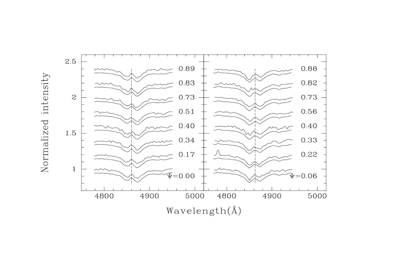
Figure 5: Evolution of the normalized H$\beta$ profile through the orbital phase. Left: February 25. Right: February 26. The dashed lines show the center of the emission cores of the average spectra, which are 4860.1 Å and 4862.9 Å, respectively. The lower line in every pair lines is the intraday average spectrum.

Figure 6: The upper two panels show the asymmetry and symmetry of H$\beta$ on February 25 and 26. The asymmetry is exactly opposite for the two days. The lower two panels show two sample-simulated H$\beta$ profiles, which are produced according to the model in the text. They reproduced all the asymmetric and symmetric features of the observed profiles.

Figure 7: Simulated dependence of the ratio of the shallower core of the absorption component to the deeper one on $\Theta$. The solid and dotted lines are for February 25 and 26, respectively. From the property that the ratio is factually larger on February 25, we know that only solution B is correct.

Figure 8: Least-squares sinusoidal fitted separately for the radial velocities of the wings of H$\beta$ of February 25 (open triangles) and 26 (solid triangles). It shows clearly that the $\gamma$ velocity of these two days varied with a amplitude of $\sim$50 km s^-1.

References

- Balayan (1997) Balayan, S. K. 1997, Ap., 40, 211
- Frank et al. (2002) Frank, J., King, A., & Raine, D. 2002, Accretion Power in Astrophysics (3rd ed; Cambridge: Cambridge Univ. Press)
- Hazen & Garnavich (1999) Hazen, M. L., Garnavich, P. M. 1999, JAAVSO, 27, 19
- Hirose & Osaki (1990) Hirose, M., & Osaki, Y. 1990, PASJ, 42, 135
- Honey et al. (1988) Honey, W. B., Charles, P. A., Whitehurst, R., Barrett, P. E., & Smale, A. P. 1988, MNRAS, 231, 1
- Horne (1995) Horne, K. 1995, A&A, 297, 273
- Kippenhahn & Weigert (1990) Kippenhahn, R., & Weigert, A. 1990, Steller Structure and Evolution (Berlin: Springer)
- Kunze et al. (1997) Kunze, S., Speith, R., & Riffert, H. 1997,MNRAS, 289, 889
- Krzeminski & Vogt (1985) Krzeminski, W., & Vogt, N. 1985, A&A, 144, 124
- Makarian & Stepanian (1983) Makarian, B. E., & Stepanian, D. A. 1999, Afz, 19, 639
- Marsh (1987) Mash, T. R. 1987, MNRAS, 228, 779
- (12) Murray, J. R. 1998, MNRAS, 297, 323
- Nogami (1998) Nogami, D. 1998, , No. 1452
- Osaki (1989) Osaki, Y. 1989, PASJ, 41, 1005
- Paczyński (1977) Paczyński, B. 1977, ApJ, 216, 822
- Patterson (2003) Patterson, J. 2001, PASP, 113, 736
- Patterson et al. (2003) Patterson, J. et al. 2003, PASP, 115, 1308
- Patterson et al. (1993) Patterson, J., Halpern, J., & Shambrook, A. 1993, ApJ, 419, 803, named Paper II in the text
- Scargel (1982) Scargle, J. D. 1982, ApJ, 263, 835
- Schoembs (1986) Schoembs, R. 1986, A&A, 158, 233
- Shafter et al. (1988) Shafter, A. W., Hessman, F. V., & Zhang, E. H. 1988, ApJ, 327. 248
- Thorstensen et al. (1996) Thorstensen, J. R., Patterson, J. O., Shambrook, A., & Thomas, G. 1996, PASP, 108, 73
- Thorstensen et al. (1991) Thorstenten, J. R., Ringwald, F.A., & Wade, R.A. 1991, 102, 272
- Truss et al. (2001) Truss, M. R., Murray, J. R., & Wynn, G. A. 2001, MNRAS, 324, L1
- Vanmunster (1998) Vanmunster, T. 1998, , No. 1448
- Vogt (1982) Vogt, N., 1982, ApJ, 252, 653
- Warner (1985) Warner, B. 1985, Interacting Binaries (Dordrecht: D. Reidel Publishing Company), p367
- Warner (1995) Warner, B. 1995, Cataclysmic Variable Stars (Cambridge: Cambridge Univ. Press)
- Whitehurst (1994) Whitehurst, R. 1994, MNRAS, 266, 35
- Wu et al. (2001) Wu, X., Li, Z. Gao, W., & Leung, K.-C. 2001, ApJ, 549, L81, named Paper I in the text