INTEGRAL  and XMM-Newton  observations of the X-ray pulsar IGR J16320$-$4751/AX J1631.9$-$4752

Abstract

We report on observations of the X-ray pulsar IGR J16320$-$4751 (a.k.a. AX J1631.9$-$4752) performed simultaneously with INTEGRAL and XMM-Newton. We refine the source position and identify the most likely infrared counterpart. Our simultaneous coverage allows us to confirm the presence of X-ray pulsations at $\sim 1300$ s, that we detect above 20 keV with INTEGRAL for the first time. The pulse fraction is consistent with being constant with energy, which is compatible with a model of polar accretion by a pulsar. We study the spectral properties of IGR J16320$-$4751 during two major periods occurring during the simultaneous coverage with both satellites, namely a flare and a non-flare period. We detect the presence of a narrow 6.4 keV iron line in both periods. The presence of such a feature is typical of supergiant wind accretors such as Vela X-1 or GX 301$-$2. We inspect the spectral variations with respect to the pulse phase during the non-flare period, and show that the pulse is solely due to variations of the X-ray flux emitted by the source and not to variations of the spectral parameters. Our results are therefore compatible with the source being a pulsar in a High Mass X-ray Binary. We detect a soft excess appearing in the spectra as a blackbody with a temperature of $\sim$0.07 keV. We discuss the origin of the X-ray emission in IGR J16320$-$4751: while the hard X-rays are likely the result of Compton emission produced in the close vicinity of the pulsar, based on energy argument we suggest that the soft excess is likely the emission by a collisionally energised cloud in which the compact object is embedded.

1 Introduction

The INTErnational Gamma-Ray Astrophysics Laboratory (INTEGRAL) was launched on October 17, 2002 (Winkler et al. 2003). Since then, through regular scans of our Galaxy and guest observers’ observations, about 75 new sources have been discovered mainly with the IBIS telescope (Ubertini et al. 2003), thanks to its low energy camera ISGRI (Lebrun et al. 2003). Because of its energy range (from 15 keV to $\sim 1$ MeV), its high angular resolution (12 arcmin), good positional accuracy (down to $\sim 0.5$ arcmin for bright sources), and its unprecedented sensitivity between 20 and 200 keV, IBIS/ISGRI has helped to answer the question of the origin of the hard X-ray background in the Galaxy (Lebrun et al., 2004). These capacities have also allowed to discover many peculiar X-ray binaries characterized by a huge equivalent absorption column density ($N_{\mathrm{H}}$), as high as a few times $10^{24}$ cm^-2 in IGR J16318$-$4848 Matt & Guainazzi (2003); Walter et al. (2003), the first source discovered by INTEGRAL. Due to the high absorption, most of these sources were not detected during previous soft X-ray scans of the Galaxy (see e.g. Kuulkers 2005 for a review).
IGR J16320$-$4751 was detected on Feb. 1, 2003, with ISGRI (Tomsick et al., 2003) as a hard X-ray source. The source was observed to vary significantly in the 15$-$40 keV energy range on time scales of $\sim 1000$ s, and was sometimes detected above 60 keV (Tomsick et al., 2003; Foschini et al., 2004). Inspection of the X-ray archives revealed that IGR J16320$-$4751 is the hard X-ray counterpart to AX J1631.9-4752, observed with ASCA in 1994 and 1997 (Sugizaki et al., 2001). Analysis of archival BeppoSAX-WFC data showed that this source was persistent for at least 8 years (in’t Zand et al. 2003). Soon after the discovery of IGR J16320$-$4751 by INTEGRAL, an XMM-Newton Target of Opportunity was triggered. This allowed us to obtain the most accurate X-ray position to date (Rodriguez et al., 2003), which in particular led to the identification of two possible infrared counterparts (Tomsick et al., 2003; Rodriguez et al., 2003) (hereafter source 1 and 2). From this analysis, we suggested that IGR J16320$-$4751 is probably a High Mass X-ray Binary (HMXB) hosting a neutron star (Rodriguez et al., 2003). This last point has been reinforced since the discovery of X-ray pulsations from this source in both XMM-Newton and ASCA observations (Lutovinov et al., 2005) with a pulse period of about 1300 s. Aharonian et al. (2005) reporting results of the survey of the inner regions of the Galaxy at very high energy with HESS, found a new source, HESS J1632$-$478, at a position coincident with IGR J16320$-$4751, but the authors suggest that this could be simply a chance coincidence. Very recently, Corbet et al. (2005) reported the discovery of strong modulations of the X-ray flux seen with Swift, that they interpreted as revealing the orbital period of the system. The period of 8.96 days that they find is compatible with the system containing an early type supergiant (Corbet et al. 2005).
We report here observations of IGR J16320$-$4751 performed simultaneously with INTEGRAL and XMM-Newton in August 2004. The sequence of observations is introduced in the following section together with technical information concerning the data reduction. Section 3 of this paper describes the results which are commented and discussed in the last part of the paper.

2 Observations and data reduction

The journal of the observations can be found in Table 1. The INTEGRAL observation results from an amalgamation of the observation of IGR J16318$-$4848 (PI Kuulkers, programme # 0220007) with that of IGR J16320$-$4751 (PI Foschini, programme # 0220014). IGR J16320$-$4751, however, remained the on-axis target for this observation.

Table 1: Journal of the observations analysed in this paper.

Satellite	Revolution	Date obs.			Prop. Id	total duration
	#	Start day	Stop day	(MJD-53000)		($\times 10^{3}$ s)
INTEGRAL	226	2004-Aug-19	2004-Aug-20	236.57–237.94	0220014& 0220007	$\sim 118$
XMM-Newton	860	2004-Aug-19	2004-Aug-20	236.55–237.14	0201700301	$\sim 51$

2.1 INTEGRAL Data Reduction

Our INTEGRAL observation was performed with the so-called hexagonal dithering pattern Courvoisier et al. (2003), which consists of a sequence of 7 pointings (called science windows, hereafter: SCW) following a hexagonal dithering on and around the position of the source. Being the on-axis target, IGR J16320$-$4751 is always in the fully coded field of view of the IBIS and SPI instruments, where the instrumental response is optimal. The INTEGRAL data were reduced using the Off-line Scientific Analysis (OSA) v 5.0, with specificities for each instrument described below.
The data from IBIS/ISGRI were first processed until production of images in the 20–40 and 40–80 keV energy ranges, with the aim of identifying the most active sources in the field. From the results of this step, we produced a catalogue of active sources which was given as an input for a second run producing images in the 20–60 and 60–200 keV energy ranges. In the latter we forced the extraction/cleaning of each of the catalogue sources in order to obtain the most reliable results for IGR J16320$-$4751 (see Goldwurm et al. 2003 for a detailed description of the IBIS software). In order to check for the presence of the 1300 s X-ray pulsations in the IBIS range, we also produced light curves with a time bin of 250 s (with the OSA5.0/ii_lc_extract v2.4.3 module) in the same energy ranges.
We produced spectra using two alternative methods. The first method is to use the standard spectral extraction from the OSA pipeline. The second method uses the individual images produced in 20 energy bins, to estimate the source count rate and build the spectrum as explained in Rodriguez et al. (2005). This second method can be used to cross check the results obtained with the standard spectral extraction. Comparison of the spectra obtained with the two methods showed no significant differences, we therefore used the spectra obtained with the standard procedure in our spectral fits. We used the standard response matrices provided with OSA 5.0, i.e. isgr_arf_rsp_0010.fits and isgr_rmf_grp_0016.fits, the latter rebinned to 20 spectral channels.
The source is not spontaneously detected by the JEM-X detector. We tentatively forced the extraction of science products at the position of IGR J16320$-$4751, but a rapid comparison with the XMM-Newton data showed that the JEM-X products were very likely contaminated by the nearby black hole candidate 4U 1630$-$47 that was in a bright soft state outburst at the time of the observation (Tomsick et al. 2005). These data were not considered further. We did not use the data from the spectrometer SPI, because the 2.5^∘ angular resolution did not allow to discriminate the emission of IGR J16320$-$4751 from that of e.g. 4U 1630$-$47 (the angular separation between the 2 sources is $\sim 40\arcmin$), or IGR J16318$-$4848 ($\sim 55\arcmin$).

2.2 XMM-Newton Data Reduction

The XMM-Newton data were reduced with the Science Analysis System (SAS) v6.1.0. Event lists for EPIC MOS Turner et al. (2001) and EPIC PN Strüder et al. (2001) cameras were obtained after processing of the ODF data with emchain and epchain. During the processing, the data were screened by rejecting periods of high background, and by filtering the bad pixels. The EPIC MOS were both operating in timing mode allowing one to obtain light curves from the central chip with 1.5 ms resolution. The EPIC PN was operating in full frame mode, allowing light curves with a time resolution as high as 73.4 ms to be obtained. For the PN camera we extracted the spectra and light curves from a 35^′′ radius circle centered on the source, while background products were extracted from a 60^′′ circular region free of sources (from the same chip).
Because of the operating mode of the MOS cameras, no background estimate can be obtained from the central chip where the source lies. A “quick look” to the lateral MOS chips has shown that the background remained negligible during the whole observation. The latter could therefore be neglected in the analysis of the MOS data. MOS light curves were hence extracted from the central chip of both cameras. For the three EPIC cameras light curves were extracted in different energy ranges (2–12 keV, 0.6–2 keV, 2–5 keV, 5–8 keV, 8–12 keV) with the highest time resolution achievable. Barycentric correction was applied to all light curves. The MOS light curves were then summed using the FTOOLS lcmath.
A redistribution response matrix and an ancillary response file for the PN spectral products were generated with rmfgen and arfgen. The resulting spectrum was fitted in XSPEC v11.3.1 Arnaud (1996) simultaneously with the spectrum obtained with INTEGRAL/ISGRI.

3 Results

3.1 Refining of the X-ray position

Given the long exposure time (Table 1) and the high flux from the source we tried to obtain a better estimate on the position in order to possibly discriminate between the 2 candidate counterparts Rodriguez et al. (2003). For this purpose we used the edetect_chain task after having extracted PN images in 5 energy ranges. The latter were further rebinned so that an image pixel had a physical size of 4.4^′′. The best position obtained with this method is RA_J2000=248.0077^∘ and DEC_J2000=-47.8742^∘ with a nominal uncertainty of $\sim 4^{\prime\prime}$. This is about 1.9^′′ from the position reported by Rodriguez et al. (2003). To cross check, we re-analysed the 2003 XMM-Newton observation with the latest calibration files available, and using the same edetect_chain in the same energy ranges. As explained in Rodriguez et al. (2003), only MOS data are available, and the data need to be filtered for soft proton flares. The best position we obtained is RA_J2000=248.0081^∘ and DEC_J2000=$-47.8741^{\circ}$. We therefore can refine the X-ray position to RA_J2000=16^h 32^m 01${}^{s}\!.$9 DEC_J2000= -47^∘ 52^′ 27^′′ with an uncertainty of $\sim 3^{\prime\prime}$ at 90$\%$ confidence. This new position suggests more strongly that the source labeled 1 in Fig. 1 is the genuine counterpart of IGR J16320$-$4751, since source 2 is now outside of the 90% error box on the X-ray position.
We compared the X-ray source positions for high significance sources (likelihood $\geq$ 200) with infrared sources from the 2MASS catalog. We found a match within $0.4\arcsec$ between the XMM-Newton source at RA_J2000=16^h 32^m 12${}^{s}\!.$306, DEC_J2000=-47^∘ 44^′ 59${}^{\prime\prime}\!.$32 and a bright 2MASS source with a K magnitude of 9.3 located at RA_J2000=16^h 32^m 12${}^{s}\!.$339, DEC_J2000=-47^∘ 44^′ 59${}^{\prime\prime}\!.$45. We found a second close match between the XMM-Newton source at RA_J2000=16^h 31^m 35${}^{s}\!.$642, DEC_J200=-47^∘ 51^′ 27${}^{\prime\prime}\!.$42 and a bright 2MASS source with a K magnitude of 9.3 located at RA_J2000=16^h 31^m 35${}^{s}\!.$634, DEC_J2000=-47^∘ 51^′ 27${}^{\prime\prime}\!.$89. Allowing a $1\arcsec$ error circle for the XMM-Newton source and taking into account the surface density of XMM-Newton sources and 2MASS sources at appropriate magnitude limits, we find that the chance probability of occurrence of these X-ray/IR source coincidences is 0.3%. This increases our confidence that the astrometry of the X-ray is correct and that we have identified the correct IR counterpart to IGR J16320$-$4751.

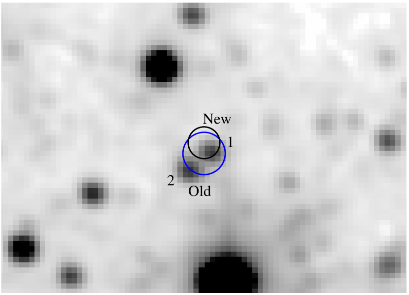
Figure 1: 2MASS K_S 1.3${}^{\prime}\times$0.9^′ image of the field around IGR J16320$-$4751. The 2 circles represent respectively the XMM-Newton position given in Rodriguez et al. (2003, large circle), and the refined position discussed in the text. Infrared sources 1 and 2 are the candidate counterparts.

3.2 Timing Analysis

The light curves of IGR J16320$-$4751 obtained in different energy ranges with the different instruments are presented in Fig. 2. As already reported, IGR J16320$-$4751 is a variable source on various time scales, from seconds-minutes (Rodriguez et al. 2003, Fig. 2), to days-months (e.g. Foschini et al. 2004). During our observations, the source shows a prominent flare around MJD 53236.6, visible in both light curves (Fig. 2). A second similar flare is visible in the ISGRI 20–60 keV light curve around MJD 53237.3. Unfortunately, our XMM-Newton observation does not cover this period.

Figure 2: Left: The 2–12 keV XMM-Newton/PN light curve of IGR J16320$-$4751. Right : The 20–60 keV INTEGRAL/ISGRI light curve of IGR J16320$-$4751. Note that the two data sets have different lengths and the light curves have different time resolutions. The time bin of the XMM-Newton light curve is 100 s, while that of INTEGRAL/ISGRI is about 3200 s (length of a SCW). Upper limits are given at the 3-$\sigma$ level.

We used the EPIC cameras to study the pulsations of IGR J16320$-$4751 already reported in Lutovinov et al. (2005). We performed a period search on the MOS and PN light curves using the XRONOS tool efsearch. Because the source is highly absorbed Rodriguez et al. (2003), and in order to improve the detection of the pulsation we restricted our period search to the 2–12 keV range for all EPIC cameras. The Lomb-Scargle of the PN 2–12 keV light curve is reported on Fig. 3.

Figure 3: Lomb-Scargle periodogram of the 2–12 keV PN light curve. The insert shows the pulse profile of the 2–12 keV light curve obtained by folding the PN light curve at a period of 1303 s.

A very prominent peak is visible with both PN and MOS detectors. Fitting the peak with Gaussian profiles lead to best values of 1303.8$\pm$0.9 s ($7.669\pm 0.005\times 10^{-4}$ Hz) and 1302.0$\pm$1.1 s ($7.680\pm 0.006\times 10^{-4}$ Hz) for MOS and PN respectively. The errors are calculated from the periodograms using the method developed by Horne & Baliunas (1986). These values are in complete agreement with the best value reported by Lutovinov et al. (2005), therefore confirming the identification of the pulsation at $\sim$1300 s.A fainter peak, is found at a period half that of the main feature (Fig. 3), that identifies it as a first harmonic of the pulse period. We then folded the PN light curve with a period of 1303 s (the mean of the of the PN and MOS values). The folded light curve is shown in Fig. 3 (insert). The pulse fraction (defined as $P=\frac{I_{max}-I_{min}}{I_{max}+I_{min}}$, where $I_{max}$ and $I_{min}$ represent respectively the intensities at the maximum and the minimum of the pulse profile) is $18.11\pm 0.7\%$ between 2 and 12 keV for the main pulse. The pulsation is also visible in the ISGRI 20–60 keV light curve. Folding the light curve at a period of 1303 s leads to a pulse fraction between 20 and 60 keV of $17\pm 4\%$. We produced light curves in several energy ranges and folded them with a period of 1303 s, in order to study the energetic dependence of the pulse fraction. As can be seen on Fig. 4 apart from the possible non-detection of pulsations below 2 keV, the pulse amplitude is compatible with being flat from 2 to 60 keV. The reported upper limit below 2 keV is 10.5%.

Figure 4: Energy dependence of the pulse fraction, obtained after folding the XMM-Newton and INTEGRAL light curves. The upper limit at low energy is given at the 3-$\sigma$ level.

3.3 Spectral Analysis

In order to avoid mixing different spectral properties together, we separated the observation in two different time regions, the first corresponding to the first flare (where we isolated $\sim 3.6$ ks), and the second corresponding to the end of the simultaneous coverage by XMM-Newton and INTEGRAL, i.e. the last $\sim 30$ ks of the XMM-Newton observation. The spectra were fitted between 0.6 and 12 keV (XMM-Newton), and 20 and 80 keV (INTEGRAL). No relative normalization constant was included in any of the fits.

3.3.1 Spectral analysis of the non-flaring period

Several models were tested in the course of the analysis starting first with phenomenological models. A single absorbed power law leads to a poor reduced $\chi^{2}$ (in the remaining of the paper $\chi^{2}_{\nu}$ stands for reduced $\chi^{2}$). In fact a large deviation is seen at high energy, indicative of a high energy cut-off. Replacing the single (absorbed) power law by a power law with a high energy cut-off improves the fit, although the $\chi^{2}_{\nu}$ is still poor, and high residuals are found around 6.4 keV. We obtain a relatively acceptable fit with a model consisting of an absorbed power law with a high energy cut-off, and a Gaussian emission line at $\sim 6.4$ keV. The $\chi^{2}_{\nu}$ is 1.48 for 441 degrees of freedom (dof). This value and some remaining significant residuals indicate that an improvement is achievable. This is particularly true below 2 keV, where a significant excess is detected, and around 7 keV. To account for the latter we included an iron edge in the model. The fit is significantly improved with $\chi^{2}_{\nu}$=1.20 (for 439 dof). The best fit parameters are reported in Table 2 (all errors on the spectral parameters are given at the 90% confidence level). The 2-10 keV unabsorbed flux is 9.22$\times 10^{-11}$ erg cm^-2 s^-1, and the 20-100 keV flux is 2.33$\times 10^{-10}$ erg cm^-2 s^-1.
The large excess still visible below 2 keV (Fig. 5) seems to be reminiscent of several of the so-called highly-absorbed sources detected by INTEGRAL (e.g. IGR J17252$-$3616, Zurita et al. 2005, IGR J16393$-$4643, Bodaghee et al. 2005), and has been seen in other X-ray Binaries containing pulsars (e.g. Hickox, Narayan & Kallman 2004). In order to try to understand its origin, we fitted the spectra with different types of absorption. The first one ($N_{\mathrm{H}}$_ext) corresponds to the absorption on the line of sight by the Galaxy and was modeled with the phabs model in XSPEC, while the second ($N_{\mathrm{H}}$) is modeled by photo-electric absorption with variable abundance cross-sections. All the abundances where frozen to the solar values except that of iron given the presence of an emission line and an absorption edge in the simple model presented earlier. The soft excess is modeled by a blackbody emission. The spectral model is phabs*(bbody+vphabs*highecut*(powerlaw+gauss)) in the XSPEC terminology. The value of the interstellar absorption ($N_{\mathrm{H}}$_ext) was fixed to the value obtained from Dickey & Lockman (1990) in the direction of the source, i.e. $N_{\mathrm{H}}$_ext=2.1$\times 10^{22}$ cm^-2 while the abundances of elements are set to solar values. The fit is good with $\chi^{2}_{\nu}$=1.13 (438 dof). The intrinsic absorption is 11.8${}_{-0.4}^{+0.5}\times 10^{22}$ cm^-2, the blackbody temperature is $0.07_{-0.01}^{+0.04}$ keV, and the iron abundance is Z_Fe=1.50${}_{-0.15}^{+0.25}$ Z_⊙. The other parameters are compatible with those returned from the previous fit. The (extrapolated) 0.01–10 keV unabsorbed flux of the blackbody (soft excess) is 3.7 $\times 10^{-10}$ erg cm^-2 s^-1, while the 0.01–100 keV unabsorbed flux of the power law component is $\sim 4.7\times 10^{-10}$ erg cm^-2 s^-1.

Figure 5: XMM-Newton/PN and INTEGRAL/ISGRI count spectra left: non-flare spectra right: flare spectra. In both cases the continuous line represents the best fit model (edge*wabs*highecut*(powerlaw+gauss) see the text for the details of the fitting). Note that the same vertical scale is used for both.

Table 2: Best fit parameters obtained from the fit to the 0.6–12 keV and 20–80 keV XMM-Newton and INTEGRAL flare and non-flare spectra with the simple phenomenological model consisting of an absorbed power law with a high energy cut-off a Gaussian and an iron edge. Errors and limits are given at the 90% confidence level.

Spectra	$N_{\mathrm{H}}$	Cut-off Energy	e-folding	$\Gamma$	Line (centroid)	Line width	Line eq. width	Edge	Max $\tau$
	($\times 10^{22}$ cm-2)	(keV)	(keV)		(keV)	(keV)	(eV)	(keV)
Non-Flare	15.5${}_{-0.6}^{+0.1}$	7.1$\pm 0.4$	13.4${}_{-0.9}^{+0.7}$	$0.24_{-0.12}^{+0.02}$	$6.409_{-0.005}^{+0.027}$	$<0.03$	$100_{-14}^{+20}$	7.21$\pm 0.04$	0.14$\pm 0.04$
Flare	11.5$\pm 0.5$	11.4${}_{-0.5}^{+0.9}$	10.1$\pm 0.7$	0.28${}_{-0.03}^{+0.07}$	6.419$\pm 0.014$	$0.046_{-0.029}^{+0.025}$	$116_{-37}^{+39}$	7.3${}_{-0.1}^{+0.3}$	0.15${}_{-0.05}^{+0.02}$

Since a cut-off power law is usually interpreted as a signature for thermal Comptonisation, we replaced the phenomenological model by a more physical model of Comptonisation (comptt, Titarchuk 1994). The choice of this model is also dictated by the fact that it gave a good representation of the XMM-Newton spectrum of a previous observation Rodriguez et al. (2003), although the lack of high energy data had prevented us from obtaining a good constraint on the temperature of the electrons. A simple absorbed comptt model (plus a Gaussian) represents the data rather well ($\chi^{2}_{\nu}$=1.54 for 442 dof), although the soft excess and an iron edge are here again clearly visible. We therefore fitted the data with a model consisting of an (externally-) absorbed blackbody plus intrinsically-absorbed Comptonisation (all abundances are set to solar values except the iron density of the local (vphabs) absorption that was left as a free parameter) and a Gaussian line (phabs(bbody+vphabs(comptt+gauss)) in XSPEC). Similarly to the previous case, $N_{\mathrm{H}}$_ext is frozen to the Galactic value along the line of sight. We obtain a good representation of the spectrum with $\chi^{2}_{\nu}$=1.15 for 438 dof. The best fit parameters are reported in Table 3, while the “$\nu$-$F_{\nu}$” spectrum is presented in Fig. 6. The blackbody (unabsorbed) bolometric flux is 2.2 $\times 10^{-10}$ erg cm^-2 s^-1, while the 0.01–100 keV unabsorbed (i.e. external plus intrinsic absorption corrected) comptt flux is 4.4 $\times 10^{-10}$ erg cm^-2 s^-1.

Table 3: Best fit parameters obtained from the fit to the 0.6–12 keV and 20–80 keV XMM-Newton and INTEGRAL flare and non-flare spectra with the physical models involving thermal Comptonisation. $N_{\mathrm{H}}$ is the absorption intrinsic to the source, kT_bb represents the temperature of the soft excess, kT_inj the temperature of the injected photon for Comptonisation and kT_e the temperature of the Comptonising cloud. Errors represent the 90% confidence level.

Spectra	$N_{\mathrm{H}}$	ZFe	kTbb	kTinj	kTe	$\tau_{\rho}$	Line (centroid)	Line width	Line eq. width
	($\times 10^{22}$ cm-2)	Z⊙	(keV)	(keV)	(keV)		(keV)	(keV)	(eV)
Non-Flare	8.9${}_{-0.7}^{+0.2}$	1.83${}_{-0.26}^{+0.30}$	$0.075_{-0.018}^{+0.024}$	$1.98_{-0.10}^{+0.15}$	8.0${}_{-0.7}^{+1.0}$	4.9${}_{-0.4}^{+0.5}$	6.411$\pm 0.006$	$<0.03$	$100_{-20}^{+24}$
Flare	7.6${}_{-1.4}^{+1.2}$	2.2${}_{-0.6}^{+0.9}$	0.075 frozen	1.30${}_{-0.24}^{+0.31}$	6.5${}_{-0.3}^{+0.4}$	9.8${}_{-1.4}^{+1.2}$	6.419${}_{-0.015}^{+0.014}$	$0.04\pm 0.02$	$112_{-44}^{+42}$

Figure 6: XMM-Newton/PN and INTEGRAL/ISGRI unfolded spectra left: non-flare spectra right: flare spectra. In both cases the continuous line represents the best fit model (phabs*(bbody+vphabs*(comptt+gauss)) see the text for the details of the fitting). Individual components are also represented. Note that the same vertical scale is used for both.

We also tried an alternative model involving partial covering by an ionised absorber (pcfabs in XSPEC). When leaving the disc temperature free to vary, non-realistic values are obtained for its normalization. We then froze $kT_{bb}$ to the best value obtained with the other models, i.e. 0.075 keV. The fit is good with $\chi^{2}_{\nu}$= 1.17 for 444 dof. The spectral parameters are compatible with those obtained with the previous model except that the intrinsic absorption is slightly higher here (Table 4). Note that the fit indicates that the central source is almost completely covered by the absorber.

Table 4: Best fit parameters from the thermal Comptonisation model, modified by a partial-covering absorber applied to the 0.6–12 keV and 20–80 keV XMM-Newton and INTEGRAL flare and non-flare spectra. Errors and limits denote the 90% confidence level. In both cases the blackbody temperature of the soft excess is frozen to 0.075 keV.

Spectra	$N_{\mathrm{H}}$	kTinj	kTe	$\tau_{\rho}$	Covering fraction
	($\times 10^{22}$ cm-2)	(keV)	(keV)		%
Non-flare	12.2$\pm 0.6$	1.5${}^{+0.05}_{-0.11}$	7.0${}^{+0.5}_{-0.4}$	6.4$\pm$0.7	$98.4_{-0.7}^{+0.3}$
Flare	9.2${}^{+1.1}_{-1.3}$	1.0$\pm 0.2$	6.6$\pm 0.2$	9.9${}_{-0.7}^{+0.5}$	$98.0_{-0.5}^{+1.8}$

3.3.2 The initial flare

We started to fit the spectra with the best (first) phenomenological model obtained in the previous case, namely an absorbed power law with a high energy cut-off, a Gaussian line and an iron edge. The $\chi^{2}_{\nu}$ is 1.06 for 439 dof. The best fit parameters are reported in Table 2, while the spectra are shown in Fig. 5 with those of the non-flare period. The 2–10 keV unabsorbed flux is 2.39$\times 10^{-10}$ erg cm^-2 s^-1, and the 20–100 keV flux is 4.20$\times 10^{-10}$ erg cm^-2 s^-1. It is interesting to note that no soft excess is obvious here, while the value of $N_{\mathrm{H}}$ has significantly decreased. It is possible that the soft excess is still present, although at a level compatible with the emission from the source (Fig. 5). This could then affect the results of the fits, in particular the value of the absorption. In order to compare with the non-flare period, we fitted the data with the same types of models. We first started with the phabs*(bbody+vphabs*highecut*(powerlaw+gauss)) model, fixing $N_{\mathrm{H}}$_ext to the Galactic value along the line of sight. Given the presence of an iron edge in the simple previous fit, we also left the iron abundance free to vary. As one could expect, the parameters of the blackbody are poorly constrained, and the values of the parameters are close to those found without the inclusion of the blackbody. In a second run, we fixed the blackbody temperature to the value found during the non-flare period ($0.07$ keV, with the phenomenological model). A good fit is achieved with $\chi^{2}_{\nu}$=1.06 (439 dof). The value of the intrinsic absorption is still lower than in the non-flare case with $N_{\mathrm{H}}$=$7.8_{-0.8}^{+0.9}\times 10^{22}$ cm^-2. The cut-off energy is now 16.2${}_{-1.7}^{+1.6}$ keV, while the folding energy is 11.8${}_{-1.1}^{+1.2}$ keV. The iron abundance is quite higher (although compatible within the errors) than in the non-flare case with Z_Fe=1.97${}_{-0.52}^{+0.64}$. The other parameters are compatible with those obtained with the simple model. We also allowed the temperature of the blackbody to vary while fixing the value of the intrinsic absorption to that found during the non-flare period (11.8$\times 10^{22}$ cm^-2). In this case, however, non credible parameters are obtained for the blackbody.
Replacing the phenomenological model by a comptt also leads to a good representation of the spectra with $\chi^{2}_{\nu}$=1.07 for 438 dof. In a first fit the blackbody parameters are left free to vary. We obtain an upper limit on the temperature of 0.11 keV (90% confidence), but the normalization is poorly constrained. We therefore froze the temperature to the best value obtained during the non-flare period (0.075 keV) and refitted the spectra. The $\chi^{2}_{\nu}$ is 1.07 for 439 dof. The best fit parameters are almost identical to those obtained when kT_bb is free to vary, and are reported in Table 3. Contrary to the phenomenological case, the $N_{\mathrm{H}}$ value obtained, is marginally compatible with the value obtained from the fit to the non flare period.
As in the non-flare case, we replaced the previous model by a model involving partial covering. Here again, to fit the soft excess well, a blackbody component is required. Since no constraints are obtained on the blackbody parameters if the blackbody temperature is left free to vary, we froze the latter to 0.075 keV. The fit is good with $\chi^{2}_{\nu}$=1.11 for 442 dof, and the best fit parameters are reported in Table 4.

3.4 Phase Resolved Spectroscopy

To study the dependence of the spectrum along the phase, we extracted PN spectra from the non-flare period in the low part of the phase diagram (hereafter low phase) and from the high part of the phase diagram (hereafter high phase) as illustrated in Fig. 7, i.e. the high phase corresponds to the time when the count rate is higher than 3.4 cts/s, while the low phase corresponds to the time when the count rate is lower than 3 cts/s. The origin of the phase is taken here as the start of the non-flare period, which we consider as the start of the good time intervals for the phase resolved spectroscopy. The shift of the phase diagram of Fig. 7 as compared to that of Fig. 3 is simply due to the fact that the origin of the phase in the former is equal to the beginning of the entire observation. Also in Fig. 7, the vertical axis is “real” mean counts per second rather than normalized ones as it is the case in Fig. 3.
We focus on the 2–12 keV energy range, since the 0.6–2 keV does not show the presence of the pulsation with a rather constraining 3-$\sigma$ upper limit of 10.5 %. We fitted the spectra directly with the phabs(vphabs(comptt+gauss)) model. The Galactic absorption ($N_{\mathrm{H}}$_ext) was again fixed to $2.1\times 10^{22}$ cm^-2. Since we only consider the XMM-Newton spectra here, no constraint can be obtained for the temperature of the Comptonising electrons. We therefore fixed $kT_{e}$ to the value obtained during the fit to the entire non-flare spectra, i.e. 7.8 keV. In both cases the fits are good with $\chi^{2}_{\nu}$=1.18 and $\chi^{2}_{\nu}$=1.01 (422 dof) for the low and high phases, respectively. The best fit parameters are reported in Table 5.

Table 5: Best fit parameters obtained from the fit to the 2–12 keV high and low phase PN spectra, with the phabs(vphabs(comptt+gauss)) model. Errors are given at the 90% level.

Spectra	$N_{\mathrm{H}}$	ZFe	kTinj	$\tau_{\rho}$	Fe Centroid	Eq. width	2-10 unabs. Flux
	($\times 10^{22}$ cm-2)	Z⊙	(keV)	(keV)	keV	eV	($\times 10^{-10}$ erg cm-2 s-1)
Low phase	9.2${}_{-0.8}^{+0.4}$	1.7$\pm 0.3$	$1.93_{-0.11}^{+0.17}$	5.1${}_{-0.6}^{+0.4}$	6.411$\pm 0.006$	104${}_{-17}^{+20}$	0.86
High phase	9.4$\pm 1.4$	1.8${}_{-0.5}^{+0.3}$	$1.9\pm 0.3$	4.8${}_{-1.5}^{+1.0}$	6.44$\pm 0.02$	72${}_{-31}^{+38}$	1.04

It is obvious from Table 5 that the spectral parameters of both the high and low phase are completely compatible. The only change is clearly related to a change of the source flux. Although the errors on the line equivalent width may indicate this parameter does not evolve with the pulse, it is interesting to note the possible decrease of this parameter by $\sim 30\%$ between the low and high phase. This may suggest that the iron is unpulsed.

4 Discussion

We report here the analysis of simultaneous XMM-Newton and INTEGRAL observations of the enigmatic source IGR J16320$-$4751. We focus on the time of strict simultaneous coverage by both satellites. We detect very significant X-ray pulsations at a period of around 1300 s confirming previous findings Lutovinov et al. (2005). The pulsation is seen in the INTEGRAL/ISGRI light curve above 20 keV. Apart from the non-detection of the pulsation below 2 keV, no particular dependence of the pulse amplitude with the energy is seen. When studying the phase dependent XMM-Newton spectra of the source (in the non-flare) period, we observe no particular spectral differences between the high-phase and low-phase spectra. In particular, the intrinsic absorption, temperature of seed photons for Comptonisation, and plasma optical depth remain relatively constant. This is compatible with a model of polar accretion by a pulsar. The modulation of the X-ray flux is due to the misalignment of the pulsar spin axis and the pulsar magnetic axis. When the pulsar magnetic axis points towards us, the X-ray flux we detect is enhanced. The pulse period would then be the spin period as already suggested by Lutovinov et al. (2005). The weak amplitude of the pulse (as compared to other absorbed source as e.g. IGR J16393$-$4643, Bodaghee et al. 2005) may indicate that the spin axis and the magnetic axis are not highly misaligned, or simply that the angle of the pulsar equator with the line of sight is quite low. The constancy of the pulse amplitude above 20 keV indicates that the Comptonised component is also pulsed. This shows that Comptonisation occurs very close to the site of production of the soft photons.
Using two independent XMM-Newton observations, we could refine the X-ray position to the source. This allowed us to further suggest that the infrared source labeled #1 in Rodriguez et al. (2003), and in Fig. 1 here was the most likely counterpart to IGR J16320$-$4751. As discussed in Rodriguez et al. (2003), the magnitudes of this object could be indicative of some infrared excess possibly due to circumstellar matter, either a hot plasma or some dust.
We provide for the first time a spectral analysis of IGR J16320$-$4751 up to 80 keV, with significant detection by INTEGRAL/ISGRI. The hard X-ray spectrum of the source is indicative of a high energy cut-off, whose parameters can not be constrained when focusing on the soft X-rays only (Rodriguez et al. 2003). The main emission mechanism in the source seems to be Compton up-scattering of soft X-ray photons by a hotter plasma. The spectral parameters we obtained either with phenomenological fits (Table 2) or more physical fits to the data are similar to those obtained for several High Mass X-ray Binaries (HMXB) (e.g. 4U 1700$-$37, Boroson et al. 2003). If we assume the source is associated with the Norma arm located between 5 and 10 kpc from the Sun, with a tangent at 8 kpc, we can estimate its bolometric luminosity. During the non-flare period, the extrapolated bolometric flux of the source is $4.12\times 10^{-10}$ erg cm^-2 s^-1. This leads to a luminosity of $3.15\times 10^{36}$ erg/s at 8 kpc, and $1.23\times 10^{36}$ (resp. $4.92\times 10^{36}$) for a distance of 5 (resp. 10) kpc. We note that this estimate of the luminosity is compatible with the typical ionising luminosity of accretion driven X-ray ($1.2\times 10^{36}$ erg/s) pulsars suggested by Bildsten et al. (1997).
Our spectral analysis allowed us to reveal the presence of a soft excess that may be indicative of an additional medium. This soft excess is well fitted with a blackbody which temperature is quite low and found around 0.07 keV. Such a soft excess seems to be commonly observed in X-ray binaries Hickox et al. (2004), and some other highly absorbed INTEGRAL sources Zurita et al. (2005); Bodaghee et al. (2005); Walter et al. (2005). This soft excess can have different origins from one system to another Hickox et al. (2004). It could be for example the signature of thermal reprocessing of the harder X-rays produced by the accretion of material onto the pulsar either by the inner boundary of an optically thick accretion disc, or by an optically thin diffuse cloud. Whatever is the exact origin of the medium responsible for the soft excess, the fact that the temperature of the soft excess is different than that of the seed photon for Comptonisation rules out a model where this medium would be contained in the Comptonising cloud. It seems difficult to consider that this medium could be the Comptonising medium giving birth to the hard X-ray emission. Given that the Comptonised component shows the pulsation with an amplitude similar to that of the soft X-rays, it is very likely that Comptonisation occurs in the close vicinity of the pulsar, the seed photons being then probably emitted by the hot surface of the compact object, and the up-scattered pulsed Comptonised component emitted by the channeled accretion flow.

Figure 7: Phase diagram of the non-flare period. Only one cycle is represented. The horizontal lines represent the limit above (respectively below) which the high phase (resp. low phase) PN spectrum has been extracted.

Given the high quality of our data and the long exposure time, we detect for the first time a narrow iron line in IGR J16320$-$4751. This kind of feature is again reminiscent in many HMXB, and is also detected in most of the highly-absorbed sources unveiled by INTEGRAL, the extreme case being IGR J16318$-$4848 Matt & Guainazzi (2003); Walter et al. (2003, 2004); Kuulkers (2005). The presence of a narrow fluorescence line, as in e.g. Vela X-1, GX 301$-$2, 4U 1700$-$37, or even Cen X-3 (e.g Boroson et al. 2003; Wojdowski et al. 2003), is usually interpreted as fluorescence of iron in a wind or circumstellar matter. This indicates that accretion occurs (at least partly) through a wind. This points towards a high mass companion in IGR J16320$-$4751 rather than a low mass one. The value of the centroid obtained during the fit to the non-flare spectra corresponds to Fe XIII (House 1969). We can estimate the distance $R$ between the irradiating source and the inner radius of the fluorescent shell using $\xi=L/(\rho\times R^{2})$, with $L$ the luminosity of the source, $\rho$ the density of the gas, and $\xi$ the ionisation parameter. From Fig. 5 of Kallman et al. (2004) we can estimate $log(\xi)<2$ therefore $\xi<100$. Knowing that $\rho\times R=$$N_{\mathrm{H}}$, we obtain

$$R>\frac{L}{N_{\mathrm{H}}\times\xi}=10^{11}~{}\mathrm{cm}\sim 0.07~{}\mathrm{AU}$$

using the value of the luminosity found assuming a distance of 5 kpc i.e. $1.23\times 10^{36}$ erg/s, and $R>0.18$ AU (resp $0.28$ AU) for a distance of 8 (resp. 10) kpc. The inner edge of the fluorescent shell seems therefore quite far from the inner accretion flow which is again compatible with the presence of an additional medium responsible for the soft excess. It is interesting to note that when leaving the iron abundance free to vary, it tends to values greater than the solar abundance (using the values of the abundance of Anders & Grevesse 1989). This could be indicative of the iron origin and the cloud itself since both seem linked. Iron could have been produced by the evolution of the proto pulsar in IGR J16320$-$4751.
Given the fact that in all the energy ranges the pulse fraction is roughly constant, it is very probable that the non-detection of the pulsation below 2 keV indicates that the X-ray flux below 2 keV, and consequently the soft excess, do not pulsate. As discussed in Hickox et al. (2004), this clearly rules out the accretion column as the origin of the soft excess. This property would suggest that the soft excess is either the emission by a collisionally energised cloud or simply the reprocessing of the hard X-rays by a diffuse cloud. In the latter case it seems quite natural to think that the absorbing material is the cloud itself. Because of energy conservation, $F_{bb}\lesssim\Delta F_{comptt}$ where $F_{bb}$ is the unabsorbed bolometric flux of the blackbody and $\Delta F_{comptt}$ the difference of the unabsorbed to the absorbed ($\sim$bolometric) flux of the Comptonised component. In the non-flare case (when the blackbody components are well constrained), our fits lead to $\Delta F_{comptt}\sim 0.4\times 10^{10}$ erg cm^-2 s^-1. The unabsorbed bolometric flux of the blackbody component is 2.2 $\times 10^{-10}$ erg cm^-2 s^-1. Hence, the origin of the black body emission cannot be due to reprocessing of the hard X-rays. The soft excess would rather be the signature of a collisionally energised cloud.
We also studied the spectral properties of the source during a flare period and compared it to the non-flare period. Although a strict comparison is rendered delicate by the presence of the soft excess which is very poorly constrained during the flare, it seems that the change during the flare is accompanied by a slight decrease of the absorption column density, while the injected temperature of the photons for Comptonisation and that of the Comptonising electrons decrease significantly. Given the degeneracy of those two parameters, the contour plots of $\tau$ vs kT_e are reported in Fig. 8 for both periods. This plot shows that the evolution of the Comptonising plasma optical depth and temperature is genuine.

Figure 8: Error contour for the optical depth $\tau$ vs. the electron temperature kT_e from the fit with the comptt model and the absorption with variable abundances. The crosses mark the location of the best values, while the contour are the 68, 90 and 99% confidence region.

The ratio of the $y$($\propto kT_{e}\tau^{2}$, e.g. Titarchuk 1994) parameters between the flare and non flare spectra is $y_{noflare}/y_{flare}$=0.30, indicating a much more efficient Compton up-scattering in the case of the flare period. The short time scale on which the flare occurs is more compatible with free-falling phenomena, rather than phenomena occuring in an accretion disc where times are of the order of the viscous time scale. This argument again points to radial accretion in IGR J16320$-$4751, therefore further suggesting that the system is a HMXB.
We note that in order to test other possibilities and explain the soft excess, a model involving partial covering was tested in the course of the analysis. However although it can lead to good results, it has to be noted that this model requires the addition of the blackbody to account for the soft excess. The result of the fits indicate that the covering of the central source of X-ray is quite high and close in both cases to its maximum value. The high values of the covering fraction would tend to confirm a picture in which the X-ray source is embedded in a dense material responsible for the soft X-ray. The fact that this covering fraction undergoes few variations between the flare and the non-flare periods seem to suggest that the flare is not caused by a huge geometrical change of this medium. This does not exclude that the flare is powered by inhomogeneities in the density of the stellar wind close to the neutron star. As the size of the region responsible for the absorption and fluorescence is of the order of the orbital radius, this is where such inhomogeneities in the wind are in fact expected. The evolution of the absorbing column density in the model involving partial covering would tend to be in agreement with a picture, where variations of the local wind density are responsible for both the variations of the column density and of the hard X-ray flux. Clearly more observations on this and other highly absorbed sources will shed light on the origin of the soft excess in accreting X-ray pulsars.

References

- Aharonian et al. (2005) Aharonian et al. (the HESS collaboration) 2005, accepted for publication in ApJ, astro-ph 0510397
- Anders & Grevesse (1989) Anders, E. & Grevesse, N. 1989, GeCoA, 53, 197
- Arnaud (1996) Arnaud, K.A. 1996, in Astronomical Data Analysis Software an Systems V, A.S.P. Conference Series, G. H. Jacoby & J. Barne eds., 101, 17.
- Bodaghee et al. (2005) Bodaghee, A., Walter, R., Zurita, et al. 2005, accepted for publication in A&A, astro-ph 0510112
- Bildsten et al. (1997) Bilsten, L., Chakrabarti, D., Chiu, J., et al. 1997, ApJS, 113, 367
- Boroson et al. (2003) Boroson, B., Vrtilek, S.D, Kallman, T., Corcoran, M. 2003, ApJ, 592, 516
- Corbet et al. (2005) Corbet, R., Barbier, L., Barthelmy, S., et al. 2005, Atel 649
- Courvoisier et al. (2003) Courvoisier, T.J.-C., Walter, R., Beckmann, V., et al. 2003, A&A, 411, L53
- Dickey & Lockman (1990) Dickey, J.M. & Lockman F.J. 1990, ARA&A, 28, 215
- Foschini et al. (2004) Foschini, L., Tomsick, J.A., Rodriguez, J., et al. 2004 in ”Proceedings of the V INTEGRAL Workshop: The INTEGRAL Universe”, eds. V. Sch nfelder, G. Lichti, and C. Winkler. ESA-SP552 (2004), p. 247.
- Goldwurm et al. (2003) Goldwurm, A., David, P., Foschini, L. et al. 2003, A&A, 411, L223
- Hickox et al. (2004) Hickox, R.C., Narayan, R. & Kallman, T.R. 2004, ApJ, 614, 881
- Horne & Baliunas (1986) Horne, J.H. & Baliunas, S.L. 1986, ApJ, 302, 757
- House (1969) House, L.L. 1969, ApJS, 18, 21
- in’t Zand et al. (2003) in’t Zand J.J.M, Ubertini P., Capitanio F., Del Santo M., 2003, IAUC 8077
- Kallman et al. (2004) Kallman, T.R., Palmeri, P., Bautista, M.A., Mendoza, C. & Krolik, J.H. 2004, ApJS, 155, 675
- Kuulkers (2005) Kuulkers, E. 2005, in “Interacting Binaries: Accretion, Evolution and Outcomes”, Eds. L.A. Antonelli, et al., Proc. of the Interacting Binaries Meeting of Cefalu, Italy, July 2004, AIP, in press/ astro-ph 0504625
- Lebrun et al. (2003) Lebrun, F., Leray, J.-P., Lavocat, P., et al. 2003, A&A, 411, L141
- Lebrun et al. (2004) Lebrun, F., Terrier, R., Bazzano, A., et al. 2004, Nature,
- Lutovinov et al. (2005) Lutovinov, A.A., Rodriguez, J., Revnivtsev, M., Shtykovskiy, P. 2005, A&A, 433, L41.
- Matt & Guainazzi (2003) Matt, G. & Guainazzi, M. 2003, MNRAS, 343, L13.
- Rodriguez et al. (2003) Rodriguez, J., Tomsick, J.A., Foschini, L., et al. 2003, A&A, 407, L41
- Rodriguez et al. (2005) Rodriguez, J., Cabanac, C., Hannikainen, D.C., et al. 2005, A&A, 432, 235
- Strüder et al. (2001) Strüder L. et al., 2001, A&A, 365, L18.
- Sugizaki et al. (2001) Sugizaki, M., Mitsuda, K., Kaneda, H., et al. 2001, ApJS, 134, 77
- Tomsick et al. (2003) Tomsick, J.A., Rodriguez, J., Foschini, L., et al. 2003, IAUC 8096
- Tomsick et al. (2005) Tomsick, J.A., Corbel, S., Goldwurm, A., Kaaret, P. 2005 ApJ, 630, 413
- Titarchuk (1994) Titarchuk, L. 1994, ApJ, 434, 570
- Turner et al. (2001) Turner, M. et al., 2001, A&A, 365, L27
- Ubertini et al. (2003) Ubertini, P., Lebrun, F., Di Cocco, G. et al. 2003, A&A, 411, L131
- Walter et al. (2003) Walter, R., Rodriguez, J., Foschini, L. et al. 2003, A&A, 411, L427
- Walter et al. (2004) Walter,R., Courvoisier, T. J.-L., Foschini, L. et al. 2004, in ”Proceedings of the V INTEGRAL Workshop: The INTEGRAL Universe”, eds. V. Sch nfelder, G. Lichti, and C. Winkler. ESA-SP552 (2004), p417
- Walter et al. (2005) Walter, R., et al. 2005, submitted to A&A
- Winkler et al. (2003) Winkler, C., Courvoisier, T.J.-L., Di Cocco, G., et al. 2003, A&A, 411, L1
- Wojdowski et al. (2003) Wojdowski, P.S.,Liedahl, D.A., Sako, M., et al. 2003, ApJ 583, 959
- Zurita et al. (2005) Zurita, J., De Cesare, G., Walter, R. et al. 2005 accepted for publication in A&A, astro-ph 0511115