Abstract

Various flame tracking techniques are often used in hydrodynamic simulations. Their use is indispensable when resolving actual scale of the flame is impossible. We show that parameters defining “artificial flame” propagation found from model systems may yield flame velocities several times distinct from the required ones, due to matter expansion being ignored in the models.

Integral effect of material expansion due to burning is incorporated into flame capturing technique (FCT) [Khokhlov(1995)]. Interpolation formula is proposed for the parameters governing flame propagation yielding 0.2% accurate speed and width for any expansion (and at least 0.01% accurate for expansions typical in type Ia supernova explosions.) Several models with simple burning rates are studied with gas expansion included. Plausible performance of the technique in simulations is discussed. Its modification ensuring finite flame width is found. Implementation suggestions are summarized, main criterion being the scheme performance being insensitive to expansion parameter (thus absence of systematic errors when the burning progresses from inner to outer layers); in this direction promising realizations are found, leading to flame structure not changing while flame evolves through the whole range of densities in the white dwarf.

1 Introduction

In modeling astrophysical flames one is often faced with the necessity to properly track discontinuity surfaces. A classical situation is simulating deflagration in a near Chandrasekhar-mass white dwarf (WD), in currently a “standard model” of Ia-type supernova (SN Ia) phenomenon. Typical width of a flame is $<1$mm [Timmes et al.(1992)], which cannot be resolved, as a total size of the box for hydrodynamic simulations is of the star scale, $>10^{8}$cm.

To get energetics right one needs somehow recreate flame geometry evolution without resolving responsible for the latter microscales. Such a problem is not untypical in physics; one hopes to mimic the processes without a cutoff (= crude grid cells, of size $\Delta$) by cleverly prescribing velocity of the flame $D_{f}(\Delta)$ and perhaps other parameters, making them cutoff-dependent, so that the resulting evolution coincided with (discretized) evolution of the exact system. At the current stage several prescriptions for $D_{f}(\Delta)$ are in use. They are based on simple physical models of hydrodynamic instability development (essentially a Rayleigh-Taylor instability modified by burning; see [Khokhlov(1994)] and [Khokhlov(1995)], where the proposed $D_{f}(\Delta)$ is also verified numerically by modeling turbulent burning in uniform gravity and grid resolving instability scale), yielding $D_{f}$ of order of turbulent velocities on scale $\Delta$, $S_{\mathrm{t}}\simeq 0.5\sqrt{\mbox{$\mathcal{A}$}g\Delta}$, $\mathcal{A}$ denoting the Atwood number for fuel–ash, $g$ being the gravitational acceleration (or its projection onto the flame normal). For more general recipes for $D_{f}$ for an arbitrary grid (giving essentially the same values for uniform Cartesian grids) see [Clement(1993), Niemeyer & Hillebrandt(1995)]; “renormalization invariance” of these prescriptions was numerically checked in [Reinecke et al.(2002)], though few details are provided. Global performance of the numerical integration scheme at different resolutions is presented in detail in [Gamezo et al.(2003), Gamezo et al.(2005)]. With $D_{f}(\Delta)$ defined as a maximum of the above $S_{\mathrm{t}}(\Delta)$ and laminar flame speed these simulations (3D with octahedral symmetry) show that the energy released at $\Delta_{\mathrm{min}}=5.2\times 10^{5}\>$cm (adaptive grid used) differs from that at $\Delta_{\mathrm{min}}=10.4\times 10^{5}\>$cm by $<8$% within the first 2 seconds after ignition (and is practically indistinguishable before $t=1.62\>$s, the moment when detonation was triggered). Perhaps, more direct checks would be desirable (this is particularly important for showing the validity of adaptive-grid simulations), but it is questionable if the program outlined in the beginning of the paragraph is workable at all in view of intrinsic non-stationarity of the problem, instabilities and numerical noise. The cited works provide evidence of this invariance in statistical sense, which seems adequate in this kind of problems. All these treatments share (in 3D, on scales $\Delta>10^{5}$ cm) a remarkable property of actual $D_{f}(\Delta)$ being insensitive to microphysics, with no direct dependence on laminar flame speed.

After having chosen the favorite prescription for $D_{f}(\Delta)$ one starts evolving the flame surface in time; basically, each element of the flame is advected by the local material velocity field plus propagates with $D_{f}$ normal to itself into the fuel. One approach (level set method, LSM) is to represent a flame surface as the zero-level of a certain function $G$: flame manifold$|_{t}=\{\mathbf{r}(t):G(\mathbf{r},t)=0\}$; one then prescribes time evolution for $G$ ensuring the needed evolution of the flame surface plus some additional physical conditions, usually taking care of $G$ not developing peculiarities hindering computations. Thus at any time the flame is infinitely thin, grid cells it intersects contain partly fuel, partly ash. While such a picture seems physically-motivated, the exact fractions of fuel/ash concentrations, fluxes, etc. are computed rather crudely, the PPM-based hydrodynamic solvers used [Woodward & Colella(1984)] spread discontinuities over several grid spacings anyway. In the present paper I will stick to another flame-tracking prescription [Khokhlov(1994)].

This flame-capturing technique (FCT) is a “physical” way of evolving the flame. On increasing dissipative terms (and, actually, reintroducing them, as the only relevant in degenerate fuel burning thermal conductivity term is negligible any far from the discontinuity) in hydrodynamic equations one broadens the flame. Hence the strategy to choose such terms so that to make the flame width equal to a few grid spacings while the flame propagation velocity having the desired value. One can then smoothly turn the dissipative terms off far from the flame. In [Khokhlov(1995)] this idea was implemented by adding an equation for conventional “fuel” concentration (denoted $1-f(\mathbf{r})$ there) to basic hydrodynamic set of equations (continuity with known sources for the species concentrations, momentum and energy),

$$\frac{\partial f}{\partial t}+\mathbf{u}\cdot\nabla f=K\nabla^{2}f+\Phi(f)$$ (1)

with the simplest second space-coordinate derivative diffusion-like term and step-function burning rate $\Phi(f)\sim\theta(f-f_{0})(1-\theta(f-1))$; $\,f\in[0;1]$, $f=0$ corresponding to pure “fuel”; u is a local gas velocity. The source term in the energy conservation equation then read $q\,df/dt$, $q$ being total heat production under burning of the fuel (C+O). $K$ and $\Phi$ were chosen as described above: dependence of the velocity of the flame (1) on $K$ and $\Phi$ was obtained by analytically solving (1) in 1 dimension, with $\mathbf{u}$ being constant, simply related to the $D_{f}$; flame width was in effect estimated crudely to be of order $\sqrt{K/R}$, its dependence on $f_{0}$ was not studied. This scheme has been used essentially verbatim by several groups since then.

Apart from an insignificant (at the value $f_{0}=0.3$ used) error in determining $D_{f}(K,\Phi)$ in [Khokhlov(1995)] there are good reasons to study system (1) further:

• As described above, the technique is quite crude. The prescription for $D_{f}$ must vary along the flame front. As applied before (see thorough description in [Khokhlov(2000)]), the only factors influencing the $D_{f}$ were local gravity and mutual orientation of the front element and gravitational field. In reality the flame structure/speed are influenced by other factors as well, even neglecting the role of thermodynamic parameters variation along the front: curvature of the front; independent of the curvature flame stretch, resulting from shear velocity gradients. Aside from these, even in 1D the above procedure has flaws. Gas velocity $\mathbf{u}$ in (1) will change significantly within the flame due to the gas expansion as a result of burning, this will make the actual flame propagation speed less than the designed $D_{f}$, based on which $K$ and $\Phi$ were constructed as described above. We suggest that the above factors affect the $D_{f}$ in some universal way, independent of the underlying microstructure; that is model system (1) must be affected in much the same way as intricately wrinkled thin flame provided the widths and velocities of resulting burning regions coincide on scale $\Delta$.

  Ultimately this study would provide one with the prescription how to modify the parameters in (1) based on local density, gravity, flame curvature, background velocity fields, etc. so that to match the response of the flame region to major hydrodynamic factors in real life.

• Apart from improving the FCT reliability this study will show the amplitude/relevance of the mentioned effects in flame systems, a matter of constant attention [Markstein 1964, Dursi et al.(2003)], and how different is the effect of these on different test systems.

In this paper I study the effect of gas expansion on different realizations of system (1) in 1D. The higher-dimensionality effects require completely different methods, the results will be reported separately. In Section 2 the problem is formulated, the numerical procedure is described. In Section 3 we qualitatively analyze the master equation (1) of FCT with matter expansion for parabolic (KPP) and step-function $\Phi(f)$; difference in flame profiles helps to formulate criteria for selecting a viable realization of (1) promising adequate performance in non-stationary simulations. Section 4 contains analytic investigation of the problem for $\Phi$ being step-function, confirms accuracy of the numerical procedure and provides much faster way of getting the parameters; a new form of the diffusion term is proposed, ensuring finite flame width. Section 5 includes simple astronomically-accurate fits for the data obtained in Sec. 4 valid for any expansion; these are then refined to the SN Ia problem, we summarize a few “best” (in our opinion) schemes, explicit prescriptions for coding are provided. We conclude in Sec. 6. Appendix contains a simple analysis of performance of the scheme in real simulations.

This work expands an earlier investigation by the author presented at FLASH Center site review (University of Chicago, Oct. 2004; unpublished), comments on the performance in non-steady simulations and approximate formulae for parameter values are added. Different from [Khokhlov(1995)] form of the diffusion term (first term on the R.H.S. of (1)) is also studied here for the first time.

2 Formulation and the numerical method

2.1 Boundary problem for finding $D_{f}[\Phi(f);\Lambda]$

In this paper we restrict ourselves to a simple one dimensional model, the one where all the quantities can be expressed algebraically as functions of the fuel concentration field only. The pressure is considered hydrostatic, as in deflagrations matter velocities are at least an order of magnitude smaller than the sound speed, apart maybe from the outer regions of the WD [Timmes et al.(1992)]. The diffusion equation we consider reads

$$\frac{\partial(\rho f)}{\partial t}+\frac{\partial(\rho fu)}{\partial x}=\rho K\frac{\partial^{2}f}{\partial x^{2}}+\rho\Phi(f),$$ (2)

$f$ being the concentration of the reaction product ($1-f$ that of the fuel), $u$ local velocity, $\rho$ density of the mixture and $K$ the diffusivity.

We are searching for self-similar solutions (all quantities depending on $x-D_{f}t$ only); as applied in FCT this means we neglect thermodynamical variables changing (w.r.t. flame position) on timescales of establishing such a steady-state burning regime. In the system of reference where the flame rests the gas velocity $u(x)$ monotonically changes from $-u_{0}-D_{f}$ as $x\to-\infty$ to $-D_{f}$ at $x=+\infty$, most of this change happening within the flame width; mass conservation allows to express $u$

$$u(x)\rho(x)=-D_{f}\rho_{0},$$ (3)

($\rho_{0}$ being the density of the fuel far ahead of the front.) Substituting the self-similar form of solution and the $\rho$

$$\frac{\rho_{0}}{\rho}=1+\frac{\gamma-1}{\gamma}\,\frac{q\rho_{0}}{P_{0}}f$$ (4)

(enthalpy conservation; ideal gas EOS used in this section, $q$ signifies the heat produced in the reaction) into (2) yields a nonlinear equation for $f$:

$$-D_{f}\frac{\rho_{0}}{\rho}\frac{df}{dx}=K\frac{d^{2}f}{dx^{2}}+\Phi(f);$$ (5)

$\Phi$ throughout stands for the burning rate. We mainly consider two model $\Phi$: [Khokhlov(1995)]

$$\Phi=\left\{\begin{array}[]{ll}R&\>\mathrm{for\ }f_{0}<f<1\\ 0&\>\mathrm{otherwise}\end{array}\right.$$ (6)

and [Kolmogorov et al.(1937)]

$$\Phi=R\,f(1-f)\quad(\mathrm{for\ }0<f<1).$$ (7)

The goal is to find eigenvalues of $D_{f}$ for the boundary problem, (5) (rewritten using (4) as

$$\frac{d}{dx}\left\{K\frac{df}{dx}+D_{f}\left(f+\frac{f^{2}}{2\Lambda}\right)\right\}=-\Phi(f),$$ (8)

for analytic consideration) with requirements

$$f(-\infty) = 1$$ (9)

$$f(+\infty) = 0$$ (10)

$$0\leq f\leq 1 \forall x\in\mathbb{R}.$$ (11)

For applications in the FCT $\Lambda$ in (8) must be chosen based on the integral density jump across the flame,

$$\Lambda=\frac{\rho_{\mathrm{ash}}}{\rho_{\mathrm{fuel}}-\rho_{\mathrm{ash}}}\equiv 0.5(\mathcal{A}^{-1}-1).$$ (12)

To typical WD densities $\rho_{\mathrm{fuel}}\in[3\times 10^{7};3\times 10^{9}]$ $g/cm^{3}$ correspond $\Lambda$ from 0.69 to 6.3 (data adapted from [Khokhlov(1995)], for 0.5C+0.5O composition).

Bearing in mind the localized character of heat production/expansion under real (Arrhenius-type) burning, it may seem logical to improve our linear (4) like

$$\frac{\rho_{0}}{\rho}=1+\frac{f-f_{0}}{\Lambda(1-f_{0})}\,\theta(f-f_{0})$$ (13)

with $\rho$ remaining unchanged in the region $f\leq f_{0}$ without burning (even though $f$ changes with $x$ due to diffusion); fuel not expanding in long diffusion tail (see below) really yields $D_{f}$ significantly less sensitive to $\Lambda$; this is accompanied with broader flames. Though the latter situation may seem more convenient there is no clear way to generalize (13) to more general $\Phi$; moreover, as shown in the Appendix, (4) is far better motivated. Below we study both models (called I and II for short) to get feeling of the sensitivity of the results to the EOS.

2.2 Numerical procedure

Upon separating $\Phi$ into a product of scale- and form-factors, $\Phi(f)=R\Phi_{0}(f)$ one may deduce the explicit dependence of $D_{f}$ (supposedly existing eigenvalues) on $R$ and $K$: namely

$$D_{f}=d\sqrt{KR},$$ (14)

where $d$ is to be found as an eigenvalue of the boundary problem for $f$ considered a function of a dimensionless coordinate

$$\chi=x\sqrt{\frac{R}{K}}$$

satisfying the following equation:

$$\frac{d^{2}f}{d\chi^{2}}+d\left(1+\frac{f}{\Lambda}\right)\frac{df}{d\chi}+\Phi_{0}(f)=0,$$ (15)

and boundary conditions like (9–11).

As (15) is invariant under translations in $\chi$ it can generically be reduced to a first order equation by rewriting it in terms of

$$p=-\frac{df}{d\chi}$$

considered a function of $f$:

$$\frac{dp}{df}-d\left(1+\frac{f}{\Lambda}\right)+\frac{\Phi_{0}(f)}{p}=0.$$ (16)

This form is used below for qualitative and numerical analysis of the problem. Corresponding boundary conditions are $p(0)=p(1)=0$. Eigenfunctions $p(f)$ are nonnegative.

To diminish the effect of singularity at $p=0$, (16) was rewritten in terms of $v=p^{2}$,

$$\frac{1}{2}\frac{dv}{df}=d\sqrt{v}(1+f/\Lambda)-\Phi_{0}(f).$$ (17)

In order not to pay extra attention to locating $v=0$ points, $\sqrt{v}$ was replaced with $\sqrt{|v|}\>$. (17) was integrated by the fourth order Runge-Kutta algorithm starting from $f=1,p=0$. Grid spacing was constant ($\Delta f=10^{-5}$ for most of the runs), except near the starting point and wherever a relative change in $v$ as a result of a single iteration exceeded $1/16$ where it was refined further.

The $d$ eigenvalue was then found for step-function $\Phi_{0}(f)$ by requiring $p|_{f=1}=0$. Namely, Newton-Raphson algorithm (see, e.g. [Press et al.(1992)]) was applied, $\frac{\partial\left(\vphantom{p^{2}}v(f=1)\right)}{\partial d}$ was found simultaneously with $p(f)$, ensuring fast convergence. $d(\Lambda=\infty)$ (found beforehand by solving (23)) was used as a seed at each new $f_{0}$ value for the first $\Lambda$ in the row, for subsequent $\Lambda$’s the previous one provided seed value for $d$; 4–13 iterations were enough to get $d$ with $10^{-8}$ precision.

3 Qualitative behavior at different burning rates

3.1 Step-function

We start with the model described by (15) with $\Phi_{0}(f)=(1-\theta(f-1))\theta(f-f_{0})$. The self-similar solution describing flame propagation we are interested in must behave as follows:

$$f=1\;\forall x<x_{1},\,\;df/dx\,(x_{1})=0,\;0<f<1\mbox{ at }x>x_{1},\;\lim\limits_{x\to\infty}f(x)=0$$ (18)

(moreover, it is monotonically decreasing, in accord with physical expectations; see typical flame profiles in Fig. 1). Proof: as any solution of (15) equal to 1 at any point with non-zero $df/d\chi$ would necessarily exceed 1 nearby, the only other possible behavior near $f=1$ would have been a solution approaching $f=1$ asymptotically as $\chi\to-\infty$. The behavior of the solution of (15) in that region would have coincided with that of the linearized equation,

$$f=\bar{c}_{1}-\chi/\bar{d}+\bar{c}_{2}\exp(-\bar{d}\chi),$$ (19)

where

$$\bar{d}=d\left(1+1/\Lambda\right).$$ (20)

The latter does not remain in the vicinity of 1 as $\chi\to-\infty$ (in fact is unbounded) for any values of the integration constants $\bar{c}_{1,2}$; the only possibility for a solution to stay in $[0;1]$ is to become identically 1 at $\chi$ smaller than some $\chi_{1}$, differentiably glued to $f$ behaving like (19) as $\chi\to\chi_{1}+$.

Similar analysis in the region where $|f|\ll 1$ yields general solution of linearized equation

$$f=c_{1}+c_{2}\exp(-d\chi),$$ (21)

which tends to 0 at $\chi\to-\infty$ iff $c_{1}=0$. This completes the proof.

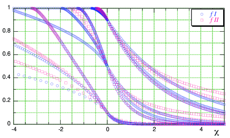
Figure 1: Flame profiles ($=$numerically found eigenfunctions). For each $f_{0}$ (the ordinate of the curve intersection with $\chi=0$) 3 pairs of profiles are depicted, for $1/\Lambda=0.05,\,4,$ and 20, larger $1/\Lambda$ corresponding to the curves intersecting $\chi=0$ axis at larger angles. Blue circles represent profiles for model I, red squares those for model II.

Summing up, the desired eigenfunction asymptotically behaves like (21) with $c_{1}=0$ as $\chi\to+\infty$, and like (19) as $\chi\to\chi_{1}+$ ($\chi_{1}=x_{1}\sqrt{R/K}$), with $\bar{c}_{1,2}$ such that

$$f(\chi_{1})=1,\;df/d\chi(\chi_{1})=0.$$ (22)

Presence of the three restrictions on the two-parameter set of functions (general solution of (15)) provides a hint that only under special circumstances does the required solution exist. As it is shown below, this actually leads to a unique value for $d$ for any fixed values of the other parameters ($\Lambda$ and $f_{0}$ here), for which there exist solutions of the boundary problem.

In the $q=0$ ($\Rightarrow\rho(x)=\rho_{0}=\mbox{const}$) case (15) actually is piecewise linear, thus the above three restrictions immediately yield $d(\Lambda=\infty,f_{0})$ as the solution of equation (cf. (30); $f(\chi_{1})$ is then expressed in elementary functions as $\Lambda=\infty$)

$$f_{0}d^{2}=1-e^{-d^{2}}.$$ (23)

One can write the solution in the limit $f_{0}\to 0$ asymptotically as $d^{2}=\frac{1}{f_{0}}-\frac{e^{-1/f_{0}}}{f_{0}}-\frac{e^{-2/f_{0}}}{f_{0}^{2}}-\left(\frac{3}{2f^{3}_{0}}+\frac{2}{f^{2}_{0}}+\frac{2}{f_{0}}\right)e^{-3/f_{0}}+O\left((f_{0}e^{1/f_{0}})^{-4}\right)$; at $f_{0}=0.3$ this yields $d$ 2% smaller than the value in [Khokhlov(1995)]; at $\Lambda$’s of interest the difference will be more significant. In the limit $f_{0}\to 1$ $d$ vanishes as $d^{2}=2(1-f_{0})+\frac{2}{3}(1-f_{0})^{2}+\frac{7}{9}(1-f_{0})^{3}+\ldots\;$(leading term agreeing with an estimate in [Zeldovich et al.(1985)], p.266).

With minor changes all said above applies to the model (13) with $\rho=\rho_{0}\;\forall f<f_{0}$, qualitative conclusions being the same.

3.2 Burning rate (7)

It is known (see [Zeldovich et al.(1985)] for detailed discussion) that the spectrum of eigenvalues of the KPP problem is continuous, comprising all reals above some $d_{1}$. In this section we show that the same holds if one includes the term arising from gas expansion, find similar spectrum for a wide range of $\Phi$’s and verify these conclusions numerically.

One can qualitatively analyze the spectrum for the burning rate (7) along the same lines as for the (6) described in the previous section. Upon linearization in the region where $1-f\ll 1$ ($\chi\to\infty$) (15) yields

$$f=1-\bar{b}_{+}e^{-\bar{\lambda}_{+}\chi}-\bar{b}_{-}e^{-\bar{\lambda}_{-}\chi},\quad{\bar{\lambda}}_{\pm}=\frac{\bar{d}}{2}\pm\sqrt{\frac{\bar{d}^{2}}{4}+1},$$ (24)

$\bar{d}=d(1+1/\Lambda)$ as before; thus there is a one parameter subset of physical solutions, those behaving asymptotically like (24) with $\bar{b}_{+}=0$.

By linearizing (15) in the region where $f\ll 1$ one gets asymptotic behavior of a solution

$$f\approx{b}_{+}e^{-{\lambda}_{+}\chi}+{b}_{-}e^{-{\lambda}_{-}\chi},\quad\lambda_{\pm}=\frac{d}{2}\pm\sqrt{\frac{d^{2}}{4}-1}.$$ (25)

There are a priori three different situations for drawing further conclusions:
1) $d<2$: any solution getting to the neighborhood of 0 necessarily becomes negative.
2) $d>2$: any $b_{+},b_{-}\geq 0$ describe physically acceptable behavior, as does a certain subset of $b_{+}<0,\;b_{-}>0$. Thus one may conjecture that for all $d>2$ there is an eigenfunction: it belongs to the described above 1-parameter subset of solutions asymptotically approaching 1 as $\chi\to-\infty$ and on becoming small at larger $\chi$ it behaves asymptotically like (25), exponentially approaching zero as $\chi\to+\infty$. Essentially, this 1-parameter set of solutions corresponds to one of them translated arbitrarily along $\chi$, i.e. there is a unique flame profile for any $d$ (the term “unique” is used below in this sense, i.e. up to translations).

One can show that the solution cannot approach any value in $(0;1)$ as $x\to+\infty$ (say, by linearizing (15) near such a value; this is of course obvious on physical grounds), and by analyzing (16) one expects the $f$ to decrease monotonically. Thus for the conjecture to fail, the solution of the above set (“physical” near 1) must have an asymptote near 0 with unphysical $b_{\pm}$ ($b_{-}<0$ in part). The numerical results below show that this does not happen and confirm the conjectured form of the flame profile.
3) $d=2$: (25) must be rewritten as $f(\chi)=(b+b_{0}\chi)e^{-\frac{d}{2}\chi}$, and there is again a 2D domain of physical $(b,b_{0})$, yielding $f>0$, $f\to 0$ as $\chi\to+\infty$. In this case a meaningful burning profile exists as well.

Analysis in this section can be straightforwardly generalized as follows:
i) If $\Phi_{0}(f)$ goes to some (positive) constant as $f\to 0$ there are no solutions going to 0 as $x\to+\infty$. From the physical viewpoint the system reacting with finite rate in the initial state is unstable and self-similar solutions cannot exist. Interestingly, some problems with $\Phi_{0}(0+)=\nu<0$ do have eigenvalues. Corresponding eigenfunctions are identically zero on the right of some $\chi_{2}$, $f(\chi)\sim\bigl{(}\nu(\chi-\chi_{2})/2\bigr{)}^{2}$ as $\chi\to\chi_{2}-$.
ii) For $\Phi_{0}(f)=\mu f+o(f)$ at $f\to 0$ non-negative solutions going to 0 as $x\to+\infty$ exist iff $d\geq 2\sqrt{\mu}$, $\mu>0$ for positiveness of $\Phi_{0}(f)$. General solution getting to a vicinity of $f=0$ decays exponentially. Analysis near $f=1\Leftrightarrow\bar{f}=1-f\ll 1$ then suggests the following for $\Phi_{0}=\bar{\nu}+\bar{\mu}\bar{f}+o(\bar{f})$ (below $d\geq 2\sqrt{\mu}$ is assumed; $f(-\infty)=1$ required):
   $\bullet$ $\bar{\nu}>0,\bar{\mu}>0$ – for all $d$ (the above $d\geq 2\sqrt{\mu}$ assumed) a unique profile exists and $\exists x_{1}:\forall x<x_{1}\;f(x)\equiv 1$.    $\bullet$ $\bar{\nu}>0,\bar{\mu}\leq 0$ – a unique profile whenever $\bar{d}\equiv d(1+\frac{1}{\Lambda})\geq 2\sqrt{-\bar{\mu}}$ (i.e. for $|\bar{\mu}|>\mu(1+1/\Lambda)^{2}$ the spectrum is additionally shrinked); again identically 1 on a half-line.
   $\bullet$ $\bar{\nu}=0,\bar{\mu}>0$ – a unique solution exponentially approaching 1 as $x\to-\infty\;\forall d$.
   $\bullet$ $\bar{\nu}=\bar{\mu}=0$. If $\Phi_{0}(f)=\bar{q}\bar{f}^{r}+o(\bar{f}^{r})$, $r>1$, $\forall d$ a unique solution exists. The solution of (16) may be written as $p=\frac{\bar{q}}{\bar{d}}\bar{f}^{r}\bigl{(}1+\frac{\bar{f}}{\Lambda+1}-\frac{r\bar{q}}{\bar{d}^{2}}\bar{f}^{r-1}+O(\bar{f}^{2}+\bar{f}^{r})\bigr{)}$, leading to $\bar{f}\sim\bigl{(}(1-r)\bar{q}\chi/\bar{d}\bigr{)}^{\frac{1}{1-r}}$. If $\Phi_{0}(f)\equiv 0$ in some neighborhood of $f=1$ bounded solutions exist but $f\to 1$ at $x\to-\infty$ from above. Not catastrophic for FCT, but unpleasant.
   $\bullet$ $\Phi_{0}\sim\bar{q}\bar{f}^{r}$, but $r\in(0;1)$. $\bar{f}$ vanishes identically on the left of some $\chi_{1}$, in its right neighborhood $\bar{f}\sim\bigl{(}\sqrt{\bar{q}/2(1+r)}(1-r)(\chi-\chi_{1})\bigr{)}^{\frac{2}{1-r}}$.
iii) For $\Phi_{0}(f)=qf^{r}$ near $f=0$ ($q>0$) there are no solutions of (16) with $p(+0)=0$ when $r<1$ – a situation analogous to i). When $r>1$ on the other hand, there are multiple solutions going to 0 (the ODE’s peculiarity), hence one expects the same behavior as in ii), depending on the $\Phi_{0}$ shape near $f=1$. When $\Phi_{0}(f)\equiv 0$ in some neighborhood of $f=0$ one would expect a discrete spectrum of $d$, with corresponding eigenfunctions behaving near $f=1$ according to the $\Phi_{0}(f)$ near 1 as in ii).

Summing this up, the KPP-like behavior is quite universal for $\Phi_{0}(f)$ going to 0 linearly or faster at $f\to 0$; on the other hand, $\Phi_{0}(f)\equiv 0$ near $f=0$ leads to the spectrum similar to that in the previous section; positive $\Phi_{0}(f)$ decreasing slower than linearly (or not going to zero) as $f\to 0$ lead to absence of steady-state solutions. Profile $f(x)$ has an infinite tail at $f=1$ iff $\Phi_{0}|_{f\to 1}$ decreases linearly or faster.

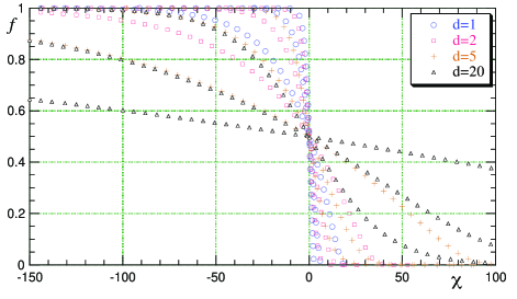
Figure 2: Flame profiles at different $\Lambda$ and $d$. For each $d$ 3 curves are depicted, for $1/\Lambda=0.05,\,5,$ and 20, larger $1/\Lambda$ corresponding to the curves intersecting $\chi=0$ axis (where $f$ was set to 0.5) at larger angles, and having larger widths.

Flame profiles $f(\chi)$ found numerically for $\Phi_{0}(f)=f(1-f)$ are shown in Fig. 2 for four values of $d$. These seem to satisfy the boundary conditions for $d\geq 2$, whereas the profiles for $d=1$ (each integrated from $p(1)\equiv-df/d\chi|_{f=1}=0$) intersect $f=0$ at finite $\chi$ with non-zero $df/d\chi$. Corresponding integral curves $p(f)$ at the same values of $d$ and $\Lambda$ are represented in Fig. 3. Note that for $d=1$  $p|_{f=0}\neq 0$, whereas for $d\geq 2$ it was checked that by refining the grid $p(0)$ became correspondingly closer to 0, down to $p(0)\approx 10^{-10}$ at the bulk grid spacing of $10^{-7}$ (at finer grid rounding errors in real(8) dominated). This numerically confirms our qualitative conclusions.

Note that the flame width grows fast with $d$. As in the original model [Kolmogorov et al.(1937)] (only asymptotes near $f=0$ are essential for the argument to hold, and these have the same exponential form regardless of $\Lambda$) one may conclude that only propagation with the smallest velocity is stable. Of course, if the $f(x)$ at some time corresponds to some eigenfunction above, such a profile will propagate with corresponding $d$. But if one considers a process of setting up the steady-state propagation, with initial $f(x)$ corresponding to pure fuel on a half-line (or $f$ decaying with $x$ faster than the fastest exponent $\lambda_{-}(d=2)=1$ in (25)) the conclusion will be that the resulting self-similar front will be the eigenfunction with the smallest velocity. More generally, by considering the evolution of some superposition $\Psi$ of the steady-state profiles found above one concludes that amplitudes of all of them but one will (asymptotically) decrease in time in favor of the one with the smallest $d$ in the spectrum of $\Psi$ (they interact due to nonlinearity of the system), decay rate being proportional to difference of corresponding $\lambda$’s. As a generic perturbation is a superposition of all the eigenfunctions, however small it is it will eventually reshuffle the profile into that for smallest $d$.

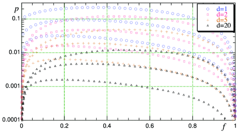
Figure 3: $p(f)$, integrated from $f=1,\,p=0$ at $\Lambda$ and $d$ as in Fig. 2; larger $1/\Lambda$ correspond to smaller $p$. Note that at $d=1$ $p(f=0)$ is non-zero, in contrast with the $d\geq 2$ curves.

It does not seem feasible to use KPP-like profile in FCT because of the continuous spectrum of the velocities, thus long times of relaxing to steady state and large widths with two exponential tails.

4 Step-function: velocities and widths

4.1 Analytic solution. Model I

Let us fix the solution (thus eliminating the translational invariance) such that $f(0)=f_{0}$. By going to dimensionless

$$\xi=d\chi=\frac{D_{f}}{K}x,\;\phi=f/\Lambda$$ (27)

and integrating once over $\xi$ one gets the first order equation for $\phi(\xi)$:

$$\frac{d\phi}{d\xi}+\phi\left(1+\frac{\phi}{2}\right)+\frac{\Phi_{0}\xi}{d^{2}\Lambda}=A.$$ (28)

Somewhat frivolous notation allows using this for two regions: where $\phi\leq f_{0}/\Lambda$ (using $\Phi_{0}=1$) and where $f_{0}/\Lambda<\phi<1/\Lambda$ ($\Phi_{0}=0$). $A$ is an integration constant, a priori different for these two regions. The boundary condition $\phi=d\phi/d\xi=0$ at $\xi=+\infty$ fixes $A=0$ for the right half-line ($\xi\geq 0$); one can further see that for model I left $A$ is zero as well, by enforcing continuous differentiability of $\phi(\xi)$ at $\xi=0$.

One can thus evaluate the flame width as (in the original units)

$$W_{1}=\frac{f_{0}}{\left|df/dx\right|_{f=f_{0}}}=\frac{K}{D_{f}}\left(1+\frac{f_{0}}{2\Lambda}\right)^{-1}=\sqrt{\frac{K}{R}}\left(d\left(1+\frac{f_{0}}{2\Lambda}\right)\right)^{-1}\equiv\sqrt{\frac{K}{R}}w_{1},$$ (29)

as well as the $\xi_{1}$ ($\xi_{1}\equiv\chi_{1}/d$ is the rightmost point where $\phi=1/\Lambda$: $\phi^{-1}(\{1/\Lambda\})=(-\infty;\xi_{1}]\,$)

$$\xi_{1}=-d^{2}\left(1+\frac{1}{2\Lambda}\right).$$ (30)

Note that the solution at positive $\xi$ is (in the original variables)

$$f=2\Lambda\left(\Bigl{(}1+\frac{2\Lambda}{f_{0}}\Bigr{)}e^{\frac{D_{f}}{K}x}-1\right)^{-1}\approx\Bigr{(}\frac{1}{2\Lambda}+\frac{1}{f_{0}}\Bigr{)}e^{-\frac{D_{f}}{K}x},$$ (31)

the last estimate is for $|x|\gg\bigl{|}\frac{K}{D_{f}}\bigr{|}\ln\bigl{(}1+{2\Lambda}/{f_{0}}\bigr{)}$; thus for small $d$ (achieved, say, at small $\Lambda$ – see below) the region where solution decays slower than asymptotic exponential is wide (may be wider than $w_{1}$ at physically reasonable parameter values), and the definition of width is ambiguous (more so taking into account complicated $f(x)$ dependence on the left half-line, cf. (35)). Therefore we will employ another definition for comparison

$$w_{2}=\frac{\chi(f=0.1)-\chi(f=1)}{0.9}$$ (32)

in numerical estimates. Analytically one finds (for $f_{0}\geq f_{-}\equiv 0.1$)

$$w_{2}=\frac{1}{d}\left(\ln\frac{1+2\Lambda/f_{-}}{1+2\Lambda/f_{0}}+d^{2}\Bigl{(}1+\frac{1}{2\Lambda}\Bigr{)}\right),$$ (33)

the first term derived from the form (31) and the second one from the above $\xi_{1}$.

In the region $(\xi_{1},0)$ one can express general solution of (28) in terms of Airy (or Bessel) functions by substitution

$$\phi=-1+\frac{2}{y}\frac{dy}{d\xi};$$ (34)

one gets

$$\phi=-1-\left(\frac{6\sigma}{d^{2}\Lambda}\right)^{1/3}\left(\frac{1}{3\sigma}+\frac{d}{d\sigma}\ln\left(\mathrm{I}_{1/3}+B\mathrm{K}_{1/3}\right)(\sigma)\right).$$ (35)

Here

$$\sigma=\left(\frac{2}{\Lambda}\right)^{1/2}\left(\xi-\frac{d^{2}\Lambda}{2}\right)^{3/2}$$ (36)

and $\mathrm{I},\mathrm{K}$ are modified Bessel functions. By imposing boundary conditions

$$\phi=\left\{\begin{array}[]{ll}f_{0}/\Lambda&\mbox{at }\sigma_{0}=d^{2}\Lambda/6\\ 1/\Lambda&\mbox{at }\sigma_{1}=\left(1+\frac{1}{\Lambda}\right)^{3}\sigma_{0}\end{array}\right.,$$ (37)

one can get the following equation, determining eigenvalues of $d$:

$$\left(\mathrm{I}_{0}\Bigl{(}1+\frac{f_{0}}{\Lambda}+\frac{1}{3\sigma_{0}}\Bigr{)}+\mathrm{I}_{0}^{\prime}\right)\left(\mathrm{K}_{1}\Bigl{(}1+\frac{1}{3\sigma_{1}}\Bigr{)}+\mathrm{K}_{1}^{\prime}\right)-\mathrm{I}\leftrightarrow\mathrm{K}=0.$$ (38)

The notation is $\mathrm{I}_{0}=\mathrm{I}_{1/3}(\sigma_{0})$, $\mathrm{K}_{1}=\mathrm{K}_{1/3}(\sigma_{1})$, etc.; the second term differs from the first one by switching functions $\mathrm{I}\leftrightarrow\mathrm{K}$, i.e. it reads $\Bigl{(}\mathrm{K}_{0}\bigl{(}1+\ldots\bigr{)}+\mathrm{K}^{\prime}_{0}\Bigr{)}\Bigl{(}\mathrm{I}_{1}\ldots\Bigr{)}$. With the above definitions this equation has a unique solution for $d$ for every $f_{0},\>\Lambda$.

4.2 Model II

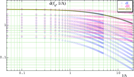
Figure 4: Flame velocities. The nine sequences $d(\Lambda)$ for each model (blue circles and red squares for model I and II respectively) correspond (top to bottom) to $f_{0}=0.1,$…0.9 with step 0.1. The worst $(f_{0}$=0.1) fit (48) for model I is shown.

In a similar way one may analyze the boundary problem with $\rho$ given by (13). ($\tilde{D}_{f}$ below denotes the eigenvalue of (5) with (9–11), $\tilde{d}$ – corresponding dimensionless speed, e.v. of (5).) One gets exponential decay of $f$ in $(0;f_{0})$, $f=f_{0}e^{-\frac{\tilde{D}_{f}}{K}x}$, the widths being

$$\tilde{W}_{1}=\textstyle{K/{\tilde{D}_{f}}},\quad\tilde{W}_{2}=\frac{K}{\tilde{D}_{f}}\left(\ln\frac{f_{0}}{f_{-}}+\tilde{d}^{2}\left(1+\frac{1-f_{0}}{2\Lambda}\right)\right).$$

The equation for

$$\tilde{\phi}(\xi)=\frac{f(\xi)-f_{0}}{\tilde{\Lambda}}\equiv\frac{f(\xi)-f_{0}}{\Lambda(1-f_{0})}$$

in the region $(\tilde{\xi}_{1};0)$,

$$\frac{d\tilde{\phi}}{d\xi}+\tilde{\phi}\Bigl{(}1+\frac{\tilde{\phi}}{2}\Bigr{)}+\frac{\Phi_{0}\xi}{d^{2}\tilde{\Lambda}}+\frac{f_{0}}{\tilde{\Lambda}}=0,$$

again has a general solution in terms of Airy functions:

$$\tilde{\phi}=-1-(\tilde{d}^{2}\tilde{\Lambda}/4)^{-1/3}\frac{d}{ds}\ln\left(\mathrm{Ai}+\tilde{B}\,\mathrm{Bi}\right)(s),$$ (39)

which after imposing the boundary conditions as above yields the equation for $\tilde{d}:$

$$\left(\mathrm{Bi}_{1}\sqrt{s_{1}}+\mathrm{Bi}^{\prime}_{1}\right)\left(\mathrm{Ai}_{0}\sqrt{\frac{s_{0}}{1-2f_{0}/\tilde{\Lambda}}}+\mathrm{Ai}^{\prime}_{0}\right)-\mathrm{Ai}\leftrightarrow\mathrm{Bi}=0.$$ (40)

In the above

$$s=-(2\tilde{d}^{2}\tilde{\Lambda})^{-1/3}\biggl{(}\xi-\frac{\tilde{d}^{2}\tilde{\Lambda}}{2}(1-2f_{0}/\tilde{\Lambda})\biggr{)},$$

and subscripts at functions again represent arguments (subscript “0” means argument $s_{0}=(\tilde{d}^{2}\tilde{\Lambda}/4)^{2/3}(1-2f_{0}/\tilde{\Lambda})$, “1” similarly implies $s_{1}=(\tilde{d}^{2}\tilde{\Lambda}/4)^{2/3}\bigl{(}1+\frac{1-f_{0}}{\tilde{\Lambda}}\bigr{)}^{2}$).

4.3 Results for velocities and widths

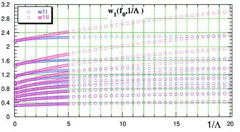
Figure 5: Flame width $w_{1}$ at the same $\Lambda$ and $f_{0}$. Larger widths correspond to larger $f_{0}$.

Numeric solutions of (40) and of (38) are presented in Fig. 4. Figs. 5 and 6 show the $w_{1}$ and $w_{2}$ for these two models. Flame profiles in Fig. 1 were obtained by direct numerical integration of (17) with the $d$ from Fig. 4. Relative difference between $d$’s found numerically and analytically is less than $5\times 10^{-3}$%. It was that large for $f_{0}\geq 0.7$; for $f_{0}\in[0.3;0.6]$ the difference was of order $10^{-8}$, the accuracy required of the $d$ in numeric procedure (that for solving (38) and (40) was set to $4\times 10^{-16}$ and apparently these errors played no role), and monotonically increased to $20\times 10^{-8}$ with $f_{0}$ further decreasing to $0.1$. Quite similar numerical integration errors were observed for model II, reaching $8.4\times 10^{-3}$% (again, with bulk integration step in $f$ being $10^{-5}$). These largest errors dropped to $10^{-3}$% when the bulk integration step was 8 times decreased. Errors in widths followed similar trends (and “numerical” widths were consistently larger than “analytical” ones, whereas velocities were smaller), though there was additional contribution from crude estimation (up to the whole grid) from integral curves $x(f)$ obtained from $p(f)$ via further trapezium integration; the discrepancy in $w_{1,2}$ in both models was less than $8\times 10^{-3}$%.

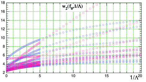
Figure 6: Flame width $w_{2}(f_{0},\Lambda)=-\chi|_{f=0.1}^{1}\Bigm{/}0.9$. For model I the order of $f_{0}$ (from larger to smaller $w_{2}$ at $1/\Lambda=20$) is 0.9, 0.1, 0.8, 0.7, 0.2, 0.6, 0.5, 0.3, $0.4\,$. That for model II is 0.1, 0.2, 0.3, 0.4, 0.9, 0.5, 0.8, 0.6, $0.7\,$.

For the problem of immediate interest (deflagration in SN Ia) matter expansion is not large, thus it is worth trying to treat $1/\Lambda$ as a small parameter. Resulting asymptotic expansion looks most natural in $h=1/d^{2}$:

$$(f_{0}-h)e^{1/h}+h - \frac{1}{2\Lambda}\left[4h+5h^{2}+e^{1/h}\left((f_{0}-h)^{2}-5h^{2}-2(f_{0}-h)\Bigl{(}1+\frac{1}{h}\Bigr{)}\right)\right.$$ (41)

$$- \left.\vphantom{e^{2/h}\frac{1}{h}}(f_{0}-h)^{2}e^{2/h}\right]+O(\Lambda^{-2})=0,$$

from which one finds a first-order correction to the solution $h_{0}\equiv d^{-2}$ of (23),

$$h=h_{0}\left(1+\frac{h_{1}}{2\Lambda}+O(\Lambda^{-2})\right),\;h_{1}=5h_{0}-e^{-1/h_{0}}\frac{2+h_{0}-h_{0}f_{0}}{f_{0}-e^{-1/h_{0}}}.$$ (42)

When $f_{0}$ is small as well this may be estimated with the aid of expansion from the end of Sec. 3.1 for $h_{0}$:

$$h_{1}=5f_{0}-e^{-1/f_{0}}\left(\frac{2}{f_{0}}+1-6f_{0}\right)-e^{-2/f_{0}}\left(\frac{4}{f_{0}^{2}}+\frac{2}{f_{0}\vphantom{f_{0}^{2}}}-6-6f_{0}\right)+O(e^{-3/f_{0}}/f_{0}^{3}),$$ (43)

this is usable up to $f_{0}\approx 0.3$. Error of using (42) does not exceed 1% for $1/\Lambda\leq 1$ (but $d=h^{-1/2}$ must be used. Expanding $d$ up to $O(1/\Lambda)$ leads to far worse agreement.) At $1/\Lambda=3$ the error grows to 6.7% for $f_{0}=0.3$ (1.8% for $f_{0}=0.2$); at $\Lambda>0.69$ (SN Ia problem) it is within 2.1% for $f_{0}=0.3$, 0.16% for $f_{0}=0.2$. At these $f_{0}$ both expressions for $h_{1}$ give the same agreement.

A very similar $1/\Lambda$ correction to (23) may be written for model II by observing that factors in front of $\tilde{\Lambda}^{0}$ and $\tilde{\Lambda}^{-1}$ under $1/\tilde{\Lambda}$ decomposition of (40) (rewritten in terms of $\mathrm{I}$ and $\mathrm{K}$ functions) coincide with the factors at the corresponding powers of $\Lambda$ in the decomposition of (38); therefore (41–43) with $\Lambda$ switched to $\tilde{\Lambda}$ provide corresponding estimates of $\tilde{d}(f_{0},\tilde{\Lambda})$.

4.4 Finite width flames

As we saw in the previous section an important drawback of KPP-like burning rates is related to exponential tails in the corresponding eigenfunctions $f(\chi)$. Behavior of the FCT models based on $\Phi_{0}(f)$ vanishing identically near $f=0$ in non-stationary simulations is better as they admit only one steady-state solution, yet for these $f(x)$ still has an infinite tail thus creating unphysically wide preheating zone in simulations hindering performance in the presence of large gradients. In this section we modify the diffusion term in (2) to make the total flame width finite.

Several possibilities have been investigated,

$$\frac{\partial(\rho f)}{\partial t}+\frac{\partial(\rho fu)}{\partial x}=\rho\frac{\partial}{\partial x}\left(\tilde{K}K_{0}(f)\frac{\partial f}{\partial x}\right)+\rho R\Phi_{0}(f)$$ (44)

with $K_{0}(f)=f^{r}$, $r\in(0;1)$ seems the simplest one providing promising results. With $\rho_{0}/\rho=1+f/\Lambda$ this problem admits a unique steady-state solution with $D_{f}=d\sqrt{\tilde{K}R}$, $d$ being the eigenvalue of

$$\frac{d}{df}\bigl{(}K_{0}(f)p\bigr{)}-d\Bigl{(}1+\frac{f}{\Lambda}\Bigr{)}+\frac{\Phi_{0}(f)}{p}=0$$ (45)

with $p(0)=p(1)=0$ (as before $p=-df/d\chi\equiv-\sqrt{\tilde{K}/R}\,df/dx$). The above $K_{0}(f)$ leads to $f(\chi)$ $C^{1}$-smoothly monotonically interpolating between $f=1\>\forall\chi<\chi_{1}=-d(1+1/2\Lambda)$ (fixing $f(0)=f_{0}$; $f=1-(\chi-\chi_{1})^{2}/2+d(\chi-\chi_{1})^{3}/2+\ldots$ at $\chi\to\chi_{1}+$) and $f=0\>\forall\chi>\chi_{2}$ ($f=(rd(\chi_{2}-\chi))^{1/r}(1+O(\chi_{2}-\chi))$ at $\chi\to\chi_{2}-$).

$\chi_{2}$ and the total width $w_{3}=\chi_{2}-\chi_{1}$ may be expressed in elementary functions of $f_{0}$, $\Lambda$ and $d$ for rational $r$ (or as incomplete $\Gamma-$function in general). Values $r=1/2$ and $r=3/4$ seem most adequate. Corresponding widths are

$$w_{3,\frac{1}{2}} = \frac{1}{d}\int_{0}^{f_{0}}f^{r-1}\left(1+\frac{f}{2\Lambda}\right)^{-1}\,df\biggr{|}_{r=1/2}-\chi_{1}=\frac{2}{d}\sqrt{2\Lambda}\arctan\sqrt{\frac{f_{0}}{2\Lambda}}+d\left(1+\frac{1}{2\Lambda}\right)$$ (46)

$$w_{3,\frac{3}{4}} = 2^{5/4}\Lambda^{3/4}d^{-1}\left[\textrm{Arctan}\,\frac{(2f_{0}/\Lambda)^{1/4}}{1-(f_{0}/2\Lambda)^{1/2}}+\ln\frac{(f_{0}/2\Lambda)^{1/2}-(2f_{0}/\Lambda)^{1/4}+1}{(f_{0}/2\Lambda+1)^{1/2}}\right]+d\left(1+\frac{1}{2\Lambda}\right)$$ (47)

In the last expression the branch of Arctan used is Arctan$\,\in[0;\pi)$.

For any $r$ in the limit $\Lambda\to\infty$

$$w_{3,r} = \frac{f_{0}^{r}}{dr}\left(1-\frac{f_{0}}{2\Lambda}\,\frac{r}{r+1}+\Bigl{(}\frac{f_{0}}{2\Lambda}\Bigr{)}^{2}\,\frac{r}{r+2}+O\Bigl{(}\frac{f_{0}}{2\Lambda}\Bigr{)}^{3}\right)+d\Bigl{(}1+\frac{1}{2\Lambda}\Bigr{)}$$

$$= \Bigl{(}\frac{f_{0}^{r}}{rd_{0}}+d_{0}\Bigr{)}+\frac{1}{2\Lambda}\left(d_{0}\Bigl{(}1-\frac{h_{1}}{2}\Bigr{)}-\frac{f_{0}^{r}}{rd_{0}}\Bigl{(}\frac{f_{0}r}{r+1}-\frac{h_{1}}{2}\Bigr{)}\right)+O(\Lambda^{-2})$$

(as in the $r=0$ case $d(f_{0},r|\Lambda)\equiv h^{-1/2}=d_{0}(1+\frac{h_{1}}{2\Lambda}+\ldots)^{-1/2}$; $d_{0}=h_{0}^{-1/2}$, $h_{1}$, etc. are now some functions of $f_{0}$ and $r$); as $\Lambda\to 0$ $w_{3}$ diverges as

$$w_{3,r}=\frac{(2\Lambda)^{r}}{d}\,\frac{\pi}{\sin\pi r}-\frac{f_{0}^{r-1}}{1-r}\,\frac{2\Lambda}{d}+O(\Lambda^{r})-\chi_{1}=\frac{2^{r}\pi}{G_{0}\sin\pi r}\Lambda^{r-1}(1-G_{1}\Lambda)+\frac{G_{0}}{2}-\frac{2}{G_{0}}\,\frac{f_{0}^{r-1}}{1-r}+O(\Lambda).$$

We used $d=G_{0}\Lambda(1+G_{1}\Lambda+o(\Lambda))$ as in the step-function model with a standard diffusion term: $d(\Lambda)$ dependence is qualitatively very similar. The fits of $d(\Lambda)$ for $r=3/4$ and various $f_{0}$ are presented in the next section.

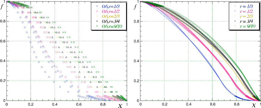
Figure 7: Normalized to unit width flame profiles with $f_{0}=0.6$ (left) and $f_{0}=0.2$ (right). The three curves for each $r$ correspond to $1/\Lambda\in\{0.16;0.6;3\}$, lower near $f=0$ profiles for larger $1/\Lambda$.

For a range of $\{f_{0},r\}$ flame profiles deliver what they were expected to originally. Their width $w_{3}$ may consistently serve as a measure of $f$ gradients, and upon coupling (44) to the hydrodynamic equations one would really get reasonably uniform heat release within the flame width. On the contrary, for the models with traditional diffusion term $w_{2}$ was somewhat arbitrary quantity, most of it (for larger $f_{0}$ and KPP to a greater degree) might correspond to “tails” of a profile, and the heat release in FCT would remain localized, contrary to the intention to more-or-less uniformly distribute it over a few cells near the modelled flame front. Some representative flame profiles are shown in Fig. 7; they are normalized to unit width (that is, reexpressed in terms of a new $X=(\chi-\chi_{1})/(\chi_{2}-\chi_{1})$; resulting supp$(df/dX)=[0;1]$); they illustrate our “top 3 picks” to be used in SN Ia simulations:
   $\bullet$ $r=1/2$. This has advantage that $f(x)$ behavior near $f=0$ is the same as near $f=1$, thus we are unlikely to introduce new problems (compared to the original $r=0$ scheme). $f_{0}=0.2$ is then convenient as the $f(x)$ shape is least sensitive to $\Lambda$ in its range of immediate interest, $1/\Lambda\in[0;2]$.
   $\bullet$ $r=3/4$, $f_{0}=0.6$. For the $\Lambda$’s of interest corresponding flame profiles seem most symmetric overall w.r.t. $f\mapsto 1-f$; this is perhaps a better realization of the above idea: as the whole $w_{3}$ width will be modelled by 3–4 integration cells this approximate global symmetry seems more adequate to consider than the symmetry of minute regions near $f=0$ and $f=1$.
   $\bullet$ $r=3/4$, $f_{0}=0.2$. Profile gradients are still uniform enough on $[0.1;0.9]$, they drop to zero in a regular manner within reasonable $\Delta\chi\leq 0.25w_{3}$. At $f_{0}=0.2$ the profiles seem least sensitive to $\Lambda$, ensuring consistent performance in all regions of the star.

5 Implementation suggestions

Analytically found asymptotes for $d(\Lambda)$ (Sec. 4.3) at small $1/\Lambda$ do not provide enough accuracy to be used for flame tracking in the outer layers of WD. Next order in $1/\Lambda$ seems marginally sufficient at $f_{0}\leq 0.2$ yet computations become too involved in $r\neq 0$ case (Sec. 4.4). More importantly, flame capturing as presented is a general method, thus it is desirable to get results with larger range of validity in a ready to use form. In this section we present fits neatly interpolating between small and large $\Lambda$ regions and then summarize the procedure for getting $K$ ($\tilde{K}$) and $R$ for (1) (respectively (44)) in the SN Ia simulations.

For model I and its modification in Sec. 4.4

$$d(\Lambda)=\frac{m_{1}}{1+m_{2}/\Lambda}+\frac{m_{3}}{(1+m_{4}/\Lambda)^{2}}$$ (48)

with $m_{1\ldots 4}$ obtained at each $f_{0}$ to minimize the mean square deviation (with weights proportional to actual $d(\Lambda)$) was the simplest fit found. The values shown in the graph below guarantee 0.2% accuracy for each $f_{0}\in\{0.01;0.025(0.025)0.975\}$ and $\Lambda\in[10^{-3};10^{5}]$ studied (for any $\Lambda$ in fact, as comparison of asymptotes shows). For $f_{0}>0.3$ agreement is significantly better.

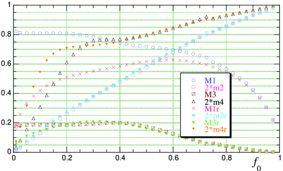
Figure 8: Fit (48) parameters for $r=0$ and $r=3/4$ (the last 4 curves according to the legend). $M_{1,3}=m_{1,3}\sqrt{f_{0}}$.

I have not succeeded to find a simple expression for $m_{1\ldots 4}(f_{0})$ providing good agreement for all expansions; this is due to delicate interplay between the two terms near $1/\Lambda=0$. To overcome this a number of other possible fits were tested. In short, 3-parameter fits were significantly less accurate (though 3% accuracy was achieved, uniformly on $\Lambda\in(0;\infty)$), fits with more than 4 parameters did not yield significant improvements; none of accurate fits admitted simple expressions for its coefficients in terms of $f_{0}$.

This is not a major issue as $f_{0}$ is a parameter one can fix at some convenient value throughout the simulation. In [Khokhlov(1995)] $f_{0}$ was fixed at 0.3, which essentially yielded thinnest flames throughout the $\Lambda$ range in the problem. The values for $K$ and $R$ used there result in actual flame speed $D_{f}=d(f_{0},\Lambda)\sqrt{f_{0}}S$, reasonably close to $S$ at small $1/\Lambda$ and $f_{0}=0.3$ (7% smaller in the WD center, however $\sim 1.45$ times smaller when $\rho=3\times 10^{7}$, 0.5C+0.5O), and flame width $W\simeq w_{2}(f_{0},\Lambda)\beta\Delta x$; $\beta=1.5$ was used, $\Delta x$ is a grid size. Now, the prescription we advocate for normalizes width as well as the flame speed, thus the logical criterion for $f_{0}$ to suggest would be the fastest tail (near $f=0$) decay in the profile normalized to unit width $w_{2}$ (we discuss traditional FCT realization (1) here; logic is the same as in 4.4). This translates to smallest $1/w_{2}d$. This, however, can be made arbitrarily small by taking sufficiently small $f_{0}$; I would suggest to stick to $f_{0}=0.2$, as this yields $1/w_{2}d$ least sensitive to $\Lambda$ in its interval of interest, from 0.4 to $\infty$; normalized this way flame profiles also exhibit fairly low sensitivity to $\Lambda$. At smaller $f_{0}$ at small $\Lambda\,(\leq 0.5)$ profile shapes on $f\in[0.1;1]$ become rather nonlinear, making the choice of $w_{2}$ as a measure for “width” more questionable.

One can observe that $\bigl{(}m_{1}+m_{3}\bigr{)}(f_{0})$ is a significantly smoother function than both terms separately (for any $r$). This sum obviously equals $d_{0}\equiv d(f_{0},r|\Lambda=\infty)$ with stated above accuracy ($\leq 0.2$%). The latter is perfectly well-defined (and is a solution of (23) in the $r=0$ case). $d(f_{0},0|\Lambda=\infty)$ can be approximated as

$$d_{0}=\left[\left(1-f_{0}^{1.4448}\exp(0.58058(1-f_{0}^{-1})\,)\right)\Bigm{/}f_{0}\right]^{0.5},$$

with accuracy of 0.64%; for $r=1/2$ and $r=3/4$ $d_{0}=\left[2\left(1-f_{0}\right)f_{0}^{r-1}\right]^{1/2}$ provides 1.5% accurate fits.

$f_{0}$	$r\;$	$m_{1}\;\;$	$m_{2}\;\;$	$m_{3}\;\;$	$m_{4}\;\;$	$\epsilon_{d},\,10^{-4}\%$
0.1		2.9248	0.081016	0.23690	0.32153	90
0.2		1.9588	0.14574	0.26929	0.42824	66
0.3		1.4620	0.19389	0.32605	0.39759	11
0.4		1.1889	0.24193	0.30495	0.39044	6.1
0.5		1.0312	0.29358	0.23117	0.40545	11
0.6		0.90646	0.34328	0.15479	0.42613	7.2
0.9		0.44817	0.46634	0.015034	0.48381	5.3
0.2	3/4	1.1683	0.14139	0.40205	0.37378	56
0.6	3/4	0.81846	0.34834	0.14334	0.42779	9.0
0.2	1/2	1.3969	0.14439	0.35064	0.39886	52

Table 1: Parameters of fit (48). The last column shows the maximum relative discrepancy between the $d(\Lambda)$ and its fit (with $m_{1\ldots 4}$ truncated exactly as in the Table) at $\Lambda\in[1/3;20]$, $\epsilon_{d}=(|\Delta d|/d)_{\mathrm{max}}$. The first seven entries correspond to model (1), $r=0$ effectively.

The fit parameters $m_{1\ldots 4}$ for $f_{0}=0.1\ldots 0.9$, as well as for the $\{f_{0},r\}$ values suggested in 4.4 optimized for $\Lambda\in[1/3;50]$ are summarized in Table 1. The final strategy is to pick one’s favorite $f_{0}$ (or $\{f_{0},r\}$) and corresponding $m_{1\ldots 4}$ from the table; then at each computation step determine the local $\Lambda$ (12) and needed $D_{f}(\Delta)$ (based on local density, gravity, etc.); (48) then defines $d$, and (33) (respectively (46) or (47)) determines dimensionless width $w$ ($w_{2}$ or $w_{3}$). Then

$$K=\frac{D_{f}}{d}\cdotp\frac{W}{w},\quad R=\frac{D_{f}}{d}\Bigm{/}\frac{W}{w},$$ (49)

(where $W$ is a desired flame width, say 3 or 4 computational cells) will lead to a flame with the desired speed $D_{f}$ and width $W$ within the approximation adopted in this paper (see Appendix).

6 Conclusions

We studied a steady state 1D burning governed by a diffusion equation for one species (fuel) with a source term representing fuel consumption; the latter depended on fuel concentration $1-f(\in[0;1])$ only. A 3D generalization of this system is widely used as a fiducial field governing the flame position and heat release in non-steady 3D simulations. Finding correct parameters of this generalization was the principal goal of the paper.

A numerical code was written for integrating the equation and finding the flame velocity $D$ and width $W$. The problem was reduced (by factoring out artificial diffusivity and burning rate normalization) to finding dimensionless $d$ and $w$ depending on the burning rate shape $\Phi_{0}(f)$ and Atwood number $\mathcal{A}$ only. Several $\Phi_{0}$’s were studied to estimate the accuracy of the technique. The results of [Kolmogorov et al.(1937)] were generalized for the system with gas expansion, the spectrum of $d$ was found continuous as in the original paper (spectrum dependence on the $\Phi_{0}(f)$ behavior near 0 and 1 was investigated in general as well; KPP-like velocity spectrum and flame profiles were found characteristic of the burning rates decreasing linearly or faster at $f\to 0$ and 1); this was confirmed numerically. Analytic solution for two other burning rate – equation of state combinations were obtained, reducing the parameters finding to solving a transcendental equation (in Bessel functions). Taking bulk integration step of 0.001 (smaller near peculiarities) in direct integration (in $f$) was enough to ensure coincidence of the results with these analytic ones within 1% for both $d$ and $w$.

Asymptotic behavior of $d$ and $w$ at $\mathcal{A}$ near 1 (no expansion) and $\infty$ (large expansion) was established. Interpolating formulae were proposed for these quantities valid for any expansion coefficient, thus providing an efficient method for finding the parameters for the equation describing flame propagation in 3D simulations. Another variation of the scheme was proposed and studied, which reslulted in finite flame width, hence promising better performance in non-stationary simulations. Specific realizations were pointed out, effectively uniformizing flame profiles (further improvement beyond widths normalization, advocated for with any variation of (1)), thus ensuring the same performance at all stages of simulation.

Brief analysis showed that the flame shall propagate with the prescribed velocity $D_{f}$ and shall have the prescribed width $W$ with high accuracy, being insensitive to details of the actual burning rate as long as most of the energy is released within its width and as long as the matter enthalpy scaling $H\propto 1/\rho$ holds on flame width scale. This is the case in the SN Ia problem, one usually defines a “flame” for the first condition to hold, and the second one is true for the first stage of deflagration in a white dwarf (while all the effectively coupled components of the matter can be considered as ultrarelativistic gas), in which virtually all of the nuclear energy is released.

We argued that the restriction of burning rate depending on $f$ only is a good approximation; burning inside the flame in most simulations is described by accurately modeling burning out of one element, while effect of burning of other species estimated crudely. This is physical — if several reactions have comparable rates, they can be effectively described by one $f$ variable; if one reaction is significantly faster, the flame is influenced by it to a higher degree, and the approximate estimate is enough.

For the boundary case, when different reactions may be important in different flame zones (or when $H\rho$ changes significantly within the flame) actual velocity of the artificial flame speed may differ from the value based on which the FCT was modeled. One might then try to consider steady state solutions of case-specific generalizations of (1) with several species and temperature involved. As another class of effects caused by finite flame width are effects of flame curvature and matter velocity gradients on the flame propagation. These will be a subject of future publications, as will be testing of the results.

Appendix
Here I present some expectations of the FCT performance with the new parameters in real-world simulations. Basic setup is the following: the physical system consists of some reactant, its concentration denoted $g(\mathbf{r},t)$, $\mathbf{u},\rho$ denote its velocity and density fields. The burning is modeled as described in Introduction. First consider a steady state burning; in such the quantities are distributed according to (5) and (1D without loss of generality)

$$\frac{dg}{dx} = \frac{G(H,g)}{\rho_{0}D_{f}}$$ (50)

$$\frac{dH}{dx} = q\frac{df}{dx},$$ (51)

continuity equation and equation of state having been used to eliminate $u(x)$ and express burning rate of $g$ as a function of enthalpy $H$ instead of the temperature (considering the pressure constant $H$ and $g$ are the only thermodynamically independent quantities. Equation for $g$ effectively decouples because of (51) form, dictated by FCT. $g$ is generally a vector, describing concentrations of all the species modelled. In some realizations instead of (50) one simply determines $g$ as some pre-defined function of $f$, that making the analysis here more straightforward).

A crucial observation at this point is that $H=\frac{const}{\rho}$ would be enough to get (from (51)) an expression for $u$ in (2) coincident with that used in model I of Sec. 2, thus tautologically yielding the same $D$ (and then the same $W$). Rest of the equations would not matter: given $f$ (51) would determine $H(x)$, while (50) would define $g(x)$. The boundary conditions for $H$ and $g$ are satisfied automatically: gradient of $H$ tends to zero at infinities; that of $g$ behaves the same at $+\infty$, assuming as usual fast reaction rate decay at low temperatures; and $g(-\infty)=0$ for usually considered $G(H,g)\propto g^{m},m\geq 2$ and $G(H(-\infty),g(+\infty))$ not very small (otherwise no reaction proceeds). On the other hand, different $H(\rho)$ would yield different $u(x)$, and the resulting eigenvalue for $D$ might differ drastically. As a ready example consider model II of Sec. 2 for prescribing $K,R$. Suppose in reality $H$ does scale $\propto 1/\rho$. One can check that the actual flame speed will be $d_{\mathrm{II}}/d_{\mathrm{I}}$ times smaller (that is 7.6 times smaller for $f_{0}=0.9$,$\>1/\Lambda=20$); one can expect comparable discrepancy for model I used for modeling a system with $d\frac{1}{\rho}/dH|_{p=const}$ being much smaller at $H(+\infty)$ (cold fuel) than at $H(-\infty)$ (hot ash). Thus, the distribution of density within the flame is important, not just an integral jump.

Fortunately for the method, $H=\frac{4p}{\rho}$ for ideal (=non-interacting in statistical physics sense, degeneracy and statistics do not matter) ultrarelativistic gas, and the matter in WD core can reasonably be considered as such. It remains ultrarelativistic during the burning, thus making assumptions behind model I applicability fulfilled. There are no clear preferences as to what value for $f_{0}$ to use at this stage.

In non-stationary burning, (8) (which would have yielded the prescribed flame velocity, time-dependent in this case) cannot be derived from (1), $\mathbf{u}$ will explicitly depend on coordinates and time. Far from caustics though one may hope that dependence to be a small correction to $|\mathbf{u}(f)|$ from the previous paragraph. Changing cross-section of streamlines (due to flame curvature and stretch), pressure changes in the gravitational field (and thus violation of $H\rho=const$ relation) are examples of this phenomenon; quasi-steady state burning is possible in this case, and the flame speed of such is a likely real flame speed in the coupled system of hydrodynamic equations and (1). Linearizing the perturbed $\mathbf{u}$ near the flame position one might find the effect of nonstationarity being possible to model with some equivalent flame with curvature. We found the geometric effects not very pronounced, being $\leq 5\%$ for flames with radius of curvature 10 times their width and above. However this whole discussion is superficial in that conditions far from the flame may still have a strong effect on its speed, as the boundary conditions are at infinities (however the models with finite width, like those studied in Sec. 4.4, must be more robust). This was seen in Section 3, similar complications occur in the problems with flame curvature. Real field-testing of the flame evolution is needed for the final verdict.

Acknowledgements
I am grateful to Alexei Khokhlov for proposing this problem, for fruitful discussions, suggestions and encouragement during the work. This work was supported by the Department of Energy under Grant No. B523820 to the Center for Astrophysical Thermonuclear Flashes at the University of Chicago.

References

- [Timmes et al.(1992)] Timmes, F. X., & Woosley, S. E. 1992, ApJ, 396, 649
- [Khokhlov(1995)] Khokhlov, A. M. 1995, ApJ, 449, 695
- [Khokhlov(1994)] Khokhlov, A. 1994, ApJ, 424, L115
- [Clement(1993)] Clement, M. J. 1993, ApJ, 406, 651
- [Niemeyer & Hillebrandt(1995)] Niemeyer, J. C., & Hillebrandt, W. 1995, ApJ, 452, 769
- [Woodward & Colella(1984)] Woodward, P., & Colella, P. 1984, J. Comp. Phys., 54, 174
- [Von Neumann & Richtmyer(1950)] Neumann, J. Von, & Richtmyer, R. D. 1950, J. of Applied Physics, 21, 232
- [Khokhlov(2000)] Khokhlov, A. M., astro-ph/0008463
- [Reinecke et al.(2002)] Reinecke, M., Hillebrandt, W., & Niemeyer, J. C. 2002, A&A, 386, 936
- [Gamezo et al.(2005)] Gamezo, V. N., Khokhlov, A. M., & Oran, E. S. 2005, ApJ, 623, 337
- [Gamezo et al.(2003)] Gamezo, V. N., Khokhlov, A. M., Oran, E. S., Chtchelkanova, A. Y., & Rosenberg, R. O. 2003, Science, 299, 77
- [Niemeyer et al.(2002)] Niemeyer, J. C., Reinecke, M., & Hillebrandt, W., astro-ph/0203369
- [Markstein 1964] Markstein, G. H. 1964, Nonsteady Flame Propagation (New York: Pergamon Press)
- [Dursi et al.(2003)] Dursi, L. J., et al. 2003, ApJ, 595, 955; astro-ph/0306176
- [Zeldovich & Frank-Kamenetskii(1938)] Zeldovich, Ya. B., Frank-Kamenetskii, D. A. 1938, Zh. Fiz. Khim. 12, 100
- [Kolmogorov et al.(1937)] Kolmogorov, A. N., Petrovskii, I. G., & Piskunov, N. S. 1937, Bull. Moskov. Gos. Univ. Mat. Mekh., 1, 1
- [Zeldovich et al.(1985)] Zeldovich, Ya. B., et al. 1985, The Mathematical Theory of Combustion and Explosions (New York: Consultants Bureau)
- [Press et al.(1992)] Press, W. H., et al. 1992, Numerical recipes in Fortran: the art of scientific computing (New York: Cambridge University Press)