On the Detection of Magnetic Helicity

Abstract

Magnetic fields in various astrophysical settings may be helical and, in the cosmological context, may provide a measure of primordial CP violation during baryogenesis. Yet it is difficult, even in principle, to devise a scheme by which magnetic helicity may be detected, except in some very special systems. We propose that charged cosmic rays originating from known sources may be useful for this purpose. We show that the correlator of the arrival momenta of the cosmic rays is sensitive to the helicity of an intervening magnetic field. If the sources themselves are not known, the method may still be useful provided we have some knowledge of their spatial distribution.

Magnetic fields pervade all astrophysical objects ZelRuzSok ; SemSok05 and there are good theoretical reasons to believe that a weak magnetic field is present throughout the universe. In astrophysical systems the magnetic field is often helical which means that the field lines are twisted (like corkscrews), or that closed magnetic lines are linked. Mathematically, the average helicity density in a volume $V$ is defined as:

$$H=\frac{1}{V}\int_{V}d^{3}x~{}{\bf A}\cdot{\bf B}.$$

In cosmology, a number of scenarios predict the creation of a primordial field with non-zero helicity. In the scenario discussed in Refs. Vachaspati:1991nm ; Vachaspati:1994xc ; Cornwall:1997ms ; Vachaspati:2001nb , a magnetic field is produced at the electroweak phase transition. The helicity of the magnetic field is related to the cosmological baryon asymmetry arising from CP violation in the fundamental particle physics theory, and the sign of the helicity is predicted to be left-handed Vachaspati:2001nb . There are also several other scenarios for the generation of primordial helical magnetic fields that do not depend on the dynamics through a phase transition generation-helicity1 ; 2 ; 3 ; 4 ; 5 ; 6 ; 7 .

The helicity of magnetic fields in astrophysical jets can be deduced from the polarization of synchrotron radiation ensslin ; valee . In such situations, the velocity of electrons in the jets is known and this additional information is crucial to the determination of helicity. In other situations, it is much harder to find the helicity. For example, Faraday rotation only provides an estimate of the line of sight component of the magnetic field. Even by observing the Faraday rotation from different sources, the information is insufficient to estimate the helicity ensslin03 ; campanelli ; Kosowsky:2004zh . An estimate of the helicity necessarily requires sensitivity to all components of the magnetic field and hence it is a challenging theoretical problem to devise means by which it may be measured. In Ref. pogosian02 ; cdk04 ; kr05 the imprint of cosmological magnetic helicity in parity-odd cross correlations of the cosmic microwave background (CMB) fluctuations was investigated, while in Ref. kgr05 it was shown that helicity would introduce circular polarization of induced relic gravitational waves. Both these potential signatures of helicity are limited to cosmological magnetic fields since they rely on properties of the cosmic microwave background or on the cosmic gravitational wave background. Further, the signals are small for several reasons: the cosmic magnetic field is constrained to be weaker than $\sim 1$ nG, the CMB is polarized only at the 10% level, the tensor modes that enter parity-odd correlations are tiny, and the gravitational waves are extremely weak.

In the present paper, we show that correlators of the arrival momenta of charged cosmic rays from known sources carry information about the helicity of the magnetic field through which the charges propagate. The scheme has the advantage that it is not restricted to cosmological magnetic fields, and it utilizes cosmic rays which are abundant and well-studied dolag . The difficulty with our scheme is that we do not normally know the source from which an observed cosmic ray emanated. However, the scheme may be extended to situations where we have some knowledge of the distribution of sources e.g. if the sources are located within a certain region of the disk of the galaxy. We have not yet explored this possibility in detail. For the present paper, we focus on establishing an observable that is sensitive to magnetic helicity. Further work is needed to decide if the observable that we propose is practically useful.

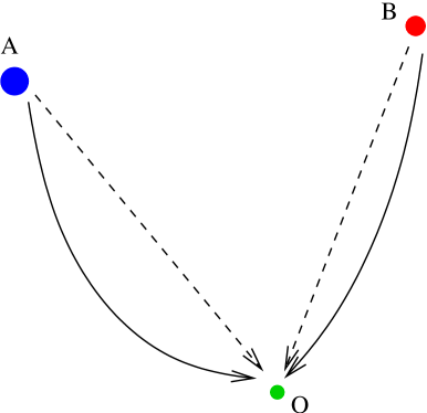
Figure 1: Two sources $A$ and $B$ emit charged particles that are observed on Earth at $O$. If there was no ambient magnetic field, the particles would follow straight trajectories (dashed lines). In the presence of a weak magnetic field, the trajectories get bent (solid curves).

Consider a situation where there are two known sources (A and B) that are emitting charged particles that arrive on Earth. The particles would propagate along straight lines from the sources to the Earth if there were no magnetic field. However, the trajectories get bent by the weak magnetic field. We work to lowest order in the magnetic field strength and consider the momenta of the particles as being perturbed due to the magnetic field:

$${\bf P}_{A}={\bf P}_{0A}+{\bf p}_{A}\ ,\ \ {\bf P}_{B}={\bf P}_{0B}+{\bf p}_{B}$$

where the $0$ in the subscript denotes an unperturbed momentum, and ${\bf p}_{A,B}$ are the momentum perturbations. The unperturbed momenta are directed along the lines of sight to the sources and the magnitudes are completely determined by the energies of the charged particles.

We are interested in the observable

$$\langle{P}_{A}^{i}(t_{f}){P}_{B}^{i^{\prime}}(t_{f}^{\prime})\rangle={P}_{0A}^{i}{P}_{0B}^{i^{\prime}}+\langle{p}_{A}^{i}(t_{f}){p}_{B}^{i^{\prime}}(t_{f}^{\prime})\rangle$$ (1)

where $i,i^{\prime}=1,2,3$ are spatial indices and $t_{f}$ and $t_{f}^{\prime}$ denote arrival times from the two sources. The ensemble average refers to an average over many realizations of the magnetic field for the same locations of the two sources. We will discuss ways in which an ensemble average can be implemented toward the end of the paper. In writing Eq. (1) we have implicitly considered particles for which the energies are fixed. Otherwise we would also have to average the unperturbed momenta since these depend on the energies of the particles. We have also taken $\langle{\bf p}_{A,B}\rangle=0$ which holds for a stochastic magnetic field with zero mean.

The first term in Eq. (1) contains the unperturbed momenta. To evaluate this contribution, it is essential that we have some knowledge of the locations of the two sources. We begin by assuming that we know the locations exactly and later comment on the case where the sources are distributed in a plane. We now evaluate the correlator for the momentum perturbations

$$C^{ii^{\prime}}=C^{ii^{\prime}}({\bf X}_{A},{\bf X}_{B})\equiv\langle{p}_{A}^{i}(t_{f}){p}_{B}^{i^{\prime}}(t_{f}^{\prime})\rangle.$$

where ${\bf X}_{A}$ and ${\bf X}_{B}$ are the vectors from $O$ to sources $A$ and $B$ respectively. We find that certain components of $C^{ii^{\prime}}$ are sensitive only to the helicity of the intervening magnetic field and vanish if the helicity is zero.

To proceed, we use the Lorentz force law to find ${\bf p}$ to linear order in the magnetic field ${\bf B}$,

$${\bf p}(t)={\bf p}_{i}+q\int_{t_{i}}^{t}dt^{\prime}~{}{\bf v}_{0}\times{\bf B}({\bf x}(t^{\prime})),$$ (2)

where we have temporarily suppressed the subscripts specifying the source for convenience. The unperturbed velocity ${\bf v}_{0}$ may be related to the unperturbed momentum using ${\bf v}_{0}={\bf P}_{0}/E$, where $E$ is the energy. The initial momentum perturbation ${\bf p}_{i}\equiv{\bf p}(t_{i})$ need not vanish and also depends on the intervening magnetic field. To determine ${\bf p}_{i}$ we integrate ${\bf P}={\bf P}_{0}+{\bf p}(t)$ over proper time

$${\bf x}(t) = {\bf x}_{i}+\frac{{\bf P}_{0}+{\bf p}_{i}}{E}(t-t_{i})$$ (3)

$$+ \frac{q}{E}\int_{t_{i}}^{t}dt^{\prime}\int_{t_{i}}^{t^{\prime}}dt^{\prime\prime}~{}{\bf v}_{0}\times{\bf B}({\bf x}(t^{\prime\prime})),$$

where ${\bf x}_{i}\equiv{\bf x}(t_{i})$ and $E$ is the energy of the particle.

We know that the charged particle arrives at the detector at $t=t_{f}$. Taking the origin of the coordinate system to be at the position of the detector, we find

$${\bf p}_{i} = -\frac{q}{T}\int_{t_{i}}^{t_{f}}dt^{\prime}\int_{t_{i}}^{t^{\prime}}dt^{\prime\prime}~{}{\bf v}_{0}\times{\bf B}({\bf x}(t^{\prime\prime}))$$ (4)

where $T\equiv t_{f}-t_{i}$ and we have used ${\bf P}_{0}=-E{\bf x}(t_{i})/T$. Going back to Eq. (2), we can write

$${\bf p}(t_{f})={\cal I}[{\bf v}_{0}\times{\bf B}({\bf x})]$$ (5)

where the action of the operator ${\cal I}$ on a function $F(t)$ is defined by

$${\cal I}[F] \equiv -\frac{q}{T}\int_{t_{i}}^{t_{f}}dt^{\prime}\int_{t_{i}}^{t^{\prime}}dt^{\prime\prime}F(t^{\prime\prime})+q\int_{t_{i}}^{t_{f}}dt^{\prime}F(t^{\prime})$$ (6)

$$= -\frac{q}{T}\int_{t_{i}}^{t_{f}}dt^{\prime}[1-T\delta(t^{\prime}-t_{f})]\int_{t_{i}}^{t^{\prime}}dt^{\prime\prime}F(t^{\prime\prime})$$

Therefore

$$C^{ii^{\prime}}={\cal I}_{A}{\cal I}_{B}\biggl{[}\epsilon_{ijk}\epsilon_{i^{\prime}j^{\prime}k^{\prime}}v_{0A}^{j}v_{0B}^{j^{\prime}}\langle B^{k}({\bf x}_{A}(t))B^{k^{\prime}}({\bf x}_{B}(t^{\prime}))\rangle\biggr{]}$$ (7)

where, for generality, we consider different species of charged particles arriving from sources $A$ and $B$ with different energies $E_{A}$, $E_{B}$ and travel times $T_{A}$, $T_{B}$.

The auto-correlator of an isotropic, stochastic, time-independent magnetic field can be written as my75

$$\langle B_{i}({\bf{x+r}})B_{j}({\bf{x}})\rangle = M_{N}(r)\left[\delta_{ij}-\frac{r_{i}r_{j}}{r^{2}}\right]+M_{L}(r)\frac{r_{i}r_{j}}{r^{2}}$$ (8)

$$+ M_{H}(r)\varepsilon_{ijl}r_{l},$$

where $M_{N}(r)$, $M_{L}(r)$, and $M_{H}(r)$ are the correlation functions for the “Normal”, “Longitudinal”, and “Helical” parts of the magnetic field. We assume that spacetime curvature can be neglected on the length scales of interest and use a Minkowski metric, so $B_{i}=-B^{i}$. All correlation functions depend only on $r=|{\bf r}|$, reflecting the statistical isotropy of the field. The divergence-less condition requires

$$M_{N}(r)=\frac{1}{2r}\frac{d}{dr}(r^{2}M_{L}(r)).$$

The ensemble averaging in Eq. (8) is over all locations ${\bf x}$ but for fixed ${\bf r}$.

The magnetic field two-point correlation function is often given in Fourier space, so it is useful to express $M_{N}(r)$, $M_{L}(r)$, and $M_{H}(r)$ in terms of a magnetic field wave number ${\bf k}$ space power spectrum defined by:

$$\langle B_{i}^{\star}({\bf{k}})B_{j}({\bf{k^{\prime}}})\rangle = (2\pi)^{3}\delta^{(3)}({\bf k}-{\bf{k^{\prime}}})$$

$$\times \left[P_{ij}{F}_{N}(k)+i\varepsilon_{ijl}\frac{k_{l}}{k}F_{H}(k)\right]$$

where the projector $P_{ij}({\mathbf{\hat{k}}})\equiv\delta_{ij}-\hat{k}_{i}\hat{k}_{j}$, and the unit vector $\hat{k}_{i}=k_{i}/k$. $F_{N}(k)$ and $F_{H}(k)$ are the symmetric and helical parts of the magnetic field power spectrum, related to the average energy density and helicity of the magnetic field. The functions $F_{N}(k)$ and $F_{H}(k)$ can be related to the correlation functions $M_{N}(r)$, $M_{L}(r)$ and $M_{H}(r)$ as in Ref. my75 .

The correlator $C^{ii^{\prime}}$, Eq. (7), may be decomposed into normal, longitudinal, and helical parts,

$$C^{ii^{\prime}}=C^{ii^{\prime}}_{N}+C^{ii^{\prime}}_{L}+C^{ii^{\prime}}_{H}$$

The remaining calculation involves inserting Eq. (8) into (7) and simplifying. Let us define

$${\bf n}={\bf v}_{0A}\times{\bf v}_{0B}.$$ (9)

A straightforward computation gives the correlator induced by the normal component of the magnetic field power spectrum,

$$C^{ii^{\prime}}_{N} = {\cal I}_{A}{\cal I}_{B}\biggl{[}M_{N}(r)\biggl{(}\delta^{ii^{\prime}}{\bf v}_{0A}\cdot{\bf v}_{0B}-{\bf v}_{0A}^{i^{\prime}}{\bf v}_{0B}^{i}$$ (10)

$$\hskip 56.9055pt-[{\bf v}_{0A}\times{\bf{\hat{r}}}]^{i}[{\bf v}_{0B}\times{\bf{\hat{r}}}]^{i^{\prime}}\biggr{)}\biggr{]}$$

where ${\bf r}(t,t^{\prime})={\bf x}_{A}(t)-{\bf x}_{B}(t^{\prime})$ and the unit vector ${\bf{\hat{r}}}={\bf r}/r$. The longitudinal piece of correlator is

$$C^{ii^{\prime}}_{L}={\cal I}_{A}{\cal I}_{B}\biggl{[}M_{L}(r)[{\bf v}_{0A}\times{\bf{\hat{r}}}]^{i}[{\bf v}_{0B}\times{\bf{\hat{r}}}]^{i^{\prime}}\biggr{]}$$ (11)

Similarly for the helical component we get:

$$C^{ii^{\prime}}_{H} = {\cal I}_{A}{\cal I}_{B}\biggl{[}M_{H}(r)\biggl{(}\epsilon^{ii^{\prime}l}[({\bf v}_{0A}\cdot{\bf r})v_{0B}^{l}+v_{0A}^{l}({\bf v}_{0B}\cdot{\bf r})]$$

$$\hskip 71.13188pt+[{r}^{i}{n}^{i^{\prime}}+{r}^{i^{\prime}}{n}^{i}]\biggr{)}\biggr{]}$$

The helical part of correlator, $C_{H}^{ii^{\prime}}$, vanishes for $i=i^{\prime}$, and the trace of the momentum perturbation correlator contains contributions only from the normal and longitudinal parts of the magnetic field spectrum:

$$C^{{\rm{TR}}} = {\cal I}_{A}{\cal I}_{B}\biggl{[}2M_{N}(r){\bf v}_{0A}\cdot{\bf v}_{0B}$$

$$\hskip-28.45274pt+(M_{L}(r)-M_{N}(r))[({\bf v}_{0A}\cdot{\bf v}_{0B})-({\bf v}_{0A}\cdot{\bf{\hat{r}}})({\bf v}_{0B}\cdot{\bf{\hat{r}}})]\biggr{]}$$

Let us take our coordinate system so that the triangle $ABO$ lies in the $xy-$plane (see Fig. 1) and ${\bf n}$ is in the ${z}-$direction. We find that all components of the helical correlator vanish except for:

$$C^{iz}_{H} = -2({\bf v}_{0B}\cdot{\bf M}_{H})({\bf v}_{0A}\times{\bf{\hat{z}}})^{i}$$ (12)

$$C^{zi}_{H} = +2({\bf v}_{0A}\cdot{\bf M}_{H})({\bf v}_{0B}\times{\bf{\hat{z}}})^{i}$$ (13)

where

$${\bf M}_{H}\equiv{\cal I}_{A}{\cal I}_{B}[M_{H}(r(t,t^{\prime})){\bf r}(t,t^{\prime})]$$ (14)

After doing the integrations, any dependence of ${\bf M}_{H}$ on $t_{f}$ and $t_{f}^{\prime}$ can be traded for a dependence on the position of the particles at the final time using: ${\bf x}_{A}(t_{f})={\bf x}_{B}(t_{f}^{\prime})=0$. A neat combination of the two components in Eqs. (12) and (13) is

$${\bf C}_{H}^{i}\equiv\frac{1}{2}[C_{H}^{iz}+C_{H}^{zi}]={\bf M}_{H}^{i}|{\bf v}_{0A}\times{\bf v}_{0B}|$$ (15)

where we have used ${\bf M}_{H}\cdot{\hat{\bf z}}=0$.

The normal component $C^{ii^{\prime}}_{N}$ vanishes if $i$ or $i^{\prime}$ (but not both) are in the ${z}-$direction. The trace of momentum correlator has the contribution only from $M_{N}$ and $M_{L}$, and in $xy-$plane $C^{\rm{Tr}}_{{\rm{xy}}}=\sum_{\alpha}C^{\alpha\alpha}$ ($\alpha=x,y$) depends only on the normal component $M_{N}(r)$,

$$C^{\rm{Tr}}_{{\rm{xy}}}={\cal I}_{A}{\cal I}_{B}[M_{N}(r)]~{}{\bf v}_{0A}\cdot{\bf v}_{0B}$$

The longitudinal component $C^{ii^{\prime}}_{L}$ vanishes if $i\neq i^{\prime}$ and has only one non-zero component when $i=i^{\prime}$ is along the $z$ direction,

$$C^{zz}_{L}={\cal I}_{A}{\cal I}_{B}\biggl{[}M_{L}(r)\{{\bf v}_{0A}\cdot{\bf v}_{0B}-({\bf v}_{0A}\cdot{\bf{\hat{r}}})({\bf v}_{0A}\cdot{\bf{\hat{r}}})\}\biggr{]}$$

On the other hand, $C^{ii^{\prime}}_{H}$ is non-zero only if one (and only one) of $i$, $i^{\prime}$ is along the $z-$direction. This can be understood on physical grounds as follows. If the magnetic field is not helical, a charged particle is as likely to be deflected in the $+z$ direction as it is to be in the $-z$ direction by the stochastic magnetic field. By symmetry, the components $C^{iz}$ must then vanish. However, a helical magnetic field breaks the symmetry and these components become non-zero. So we see that only the helical contribution enters the $xz$, $yz$, $zx$ and $zy$ components of $C^{ii^{\prime}}$, and further, only the non-helical contributions enter the other components. Therefore the normal and helical pieces of the correlator do not mix.

The other components of the correlator (e.g. $C_{xy}^{\rm{Tr}}$) can be used to find the normal and longitudinal correlation functions, $M_{N}$ and $M_{L}$. Correlations of the rotation measure due to Faraday rotation of polarized light from different sources can also be used as an independent method to determine $M_{N}$ and $M_{L}$ ensslin03 .

The above analysis relies on an average over an ensemble of random magnetic field realizations for fixed source and detector positions (triangle ABO in Fig. 1). In our universe, however, only one realization of the magnetic field is available and so we need to discuss a practical scheme for doing the ensemble average and thus estimating the correlator, $C^{ii^{\prime}}$. The ensemble average would necessarily involve averaging over many pairs of sources that we denote by $(A,B)_{\alpha}$, $\alpha=1,2,...,N$ from which we assume that cosmic rays are observed with average momenta $({\bf P},{\bf P}^{\prime})_{\alpha}$. Going back to the magnetic field correlation function, Eq. (8), we see that the ensemble average is over all ${\bf x}$ for fixed point separation ${\bf r}$. Since $C^{ii^{\prime}}$ depends on integrals of the magnetic field along the line of sight, this suggests that we find pairs of sources such that ${\bf r}(t,t^{\prime})$ is the same function of $t$ and $t^{\prime}$ for all of them. Together with the constraint that the position of the detector is fixed at O, such an ensemble has only one element and is not useful. Instead of holding ${\bf r}(t,t^{\prime})$ fixed, it is more useful to choose pairs with a less restrictive condition. There are many such possible conditions, each with its own advantage. As an example, one such condition is that the source separation vector, ${\bf\Delta}\equiv{\bf X}_{B}-{\bf X}_{A}$, be held fixed for all pairs in the ensemble. The corresponding observable is

$${\cal P}^{ii^{\prime}}({\bf\Delta})=\frac{1}{N}\sum_{\alpha=1}^{N}{\bf P}_{\alpha}^{i}{\bf P}_{\alpha}^{\prime i^{\prime}}$$ (16)

This observable quantity is an estimator for an average of the total correlator $C^{ii^{\prime}}$ discussed above, where the average is over sources with fixed separation vector $\bf\Delta$. As we have noted before, the helical part, and only the helical part, of the magnetic field enters certain components of the total correlator (see Eqs. (12) and (13)). So to get an estimator for the helical components of the correlator we should only look at those components of the estimator (16) that involve momentum in a direction in the source-observer plane and the second momentum in a direction perpendicular to this plane. Since different pairs of sources (with the same ${\bf\Delta}$) may lie in different planes, an estimator for the helical part of the correlator is

$${\cal P}_{H}({\bf\Delta})=\frac{1}{N}\sum_{\alpha=1}^{N}({\bf n}_{\alpha}\cdot{\bf P}_{\alpha})({\bf e}_{\alpha}\cdot{\bf P}_{\alpha}^{\prime})$$ (17)

where ${\bf n}_{\alpha}$ is the normal to the plane of the source pair labeled by $\alpha$ and the observer as defined in Eq. (9), and ${\bf e}_{\alpha}$ is some chosen unit vector within the plane.

To extract the magnetic helicity from a measurement of ${\cal P}_{H}({\bf\Delta})$, we must evaluate the corresponding theoretical quantity, which is given by

$${\bf\bar{C}}_{H}({\bf\Delta})=\frac{1}{V}\int_{V}d^{3}X_{A}{\bf C}_{H}({\bf X}_{A},{\bf X}_{A}+{\bf\Delta})$$

The above integral is quite involved but can be done numerically for different choices of ${\bf M}_{H}(r)$.

To summarize, a non-vanishing observed value of ${\cal P}_{H}({\bf\Delta})$ will give a measure of ${\bf\bar{C}}_{H}({\bf\Delta})$ and hence will lead to the magnetic helicity, ${\bf M}_{H}(r)$.

At present we do not have any known sources of charged cosmic rays. However, it is likely that a large fraction of cosmic rays that we see arise in the galactic disk (or sources confined in the cosmic large-scale structure ds05 ). It may be possible to usefully extend the ensemble average to include pairs of locations in the galactic disk. Such an averaging could still yield information about the helicity of the galactic magnetic field. We plan to consider this extension of our result in future work, together with other observational issues.

- (1) “Magnetic Fields in Astrophysics”, Ya. B. Zeldovich, A. A. Ruzmaikin, and D. D. Sokoloff, Gordon and Breach, New York, (1983).
- (2) V. B. Semikoz and D. D. Sokoloff, Inter. J. Mod. Phys. 14, 1839 (2005).
- (3) T. Vachaspati, Phys. Lett. B 265, 258 (1991).
- (4) T. Vachaspati, in the Proceedings of the NATO Workshop on “Electroweak Physics and the Early Universe”, Sintra, Portugal (1994); Series B: Physics Vol. 338, Plenum Press, New York (1994) [arXiv:hep-ph/9405286].
- (5) J. M. Cornwall, Phys. Rev. D 56, 6146 (1997) [arXiv:hep-th/9704022].
- (6) T. Vachaspati, Phys. Rev. Lett. 87, 251302 (2001) [arXiv:astro-ph/0101261].
- (7) M. Giovannini and M. Shaposhnikov, Phys. Rev. D 57, 2186 (1998) [arXiv:astro-ph/9710234].
- (8) G. B. Field and S. M. Carroll, Phys. Rev. D 62, 103008 (2000) [arXiv:astro-ph/9811206].
- (9) M. Giovannini, Phys. Rev. D. 61, 063004 (2000) [arXiv:astro-ph/9905358].
- (10) A. Brandenburg and E. Blackman, astro-ph/0212019.
- (11) R. Banerjee and K. Jedamzik, Phys. Rev. D 70, 123003 (2004) [arXiv: astro-ph/0410032].
- (12) V. B. Semikoz and D. D. Sokoloff, Astron. Astrophys. 433, L53 (2005) [arXiv:astro-ph/0411496].
- (13) L. Campanelli and M. Giannotti, arXiv:astro-ph/0508653.
- (14) T. A. Ensslin, Astron. & Astrophys. 401, 499 (2003).
- (15) J. P. Vallée, New Astron. Rev. 48, 763 (2004).
- (16) T. Ensslin and C. Vogt, Astron. Astrophys. 401, 835 (2003) [arXiv:astro-ph/0302426].
- (17) L. Campanelli, A. D. Dolgov, M. Giannotti, and F. L. Villante, Astrophys. J. 616, 1 (2004) [arXiv:astro-ph/0405420].
- (18) A. Kosowsky, T. Kahniashvili, G. Lavrelashvili and B. Ratra, Phys. Rev. D 71, 043006 (2005) [arXiv:astro-ph/0409767].
- (19) L. Pogosian, T. Vachaspati, and S. Winitzki, Phys. Rev. D 65, 3264 (2002) [arXiv:astro-ph/0101261].
- (20) C. Caprini, R. Durrer, and T. Kahniashvili, Phys. Rev. D 69, 063006 (2004) [arXiv:astro-ph/0304566].
- (21) T. Kahniashvili and B. Ratra, Phys. Rev. D 71, 103006 (2005) [arXiv:astro-ph/0503709].
- (22) T. Kahniashvili, G. Gogoberidze, and B. Ratra, Phys. Rev. Lett. 95, 151301 (2005) [arXiv:astro-ph/0505628].
- (23) K. Dolag, D. Grasso, V. Springel, and I. Tkachev, JETP Lett. 79, 583 (2004) [Pis’ma Zh. Eksp. Theor. Fiz., 79, 719 (2004)], [arXiv: astro-ph/0310902].
- (24) A. S. Monin and A. M. Yaglom, Statistical Fluid Mechanics: Mechanics of Turbulence, Vol. 2 (MIT Press, Cambridge, MA, 1975), Sect. 12.2.
- (25) M. Karcheiriess and D. V. Semikoz, astro-ph/0512498. .