Epicyclic oscillations of fluid bodies
Paper II. Strong gravity

Abstract

Fluids in external gravity may oscillate with frequencies characteristic of the epicyclic motions of test particles. We explicitly demonstrate that global oscillations of a slender, perfect fluid torus around a Kerr black hole admit incompressible vertical and radial epicyclic modes. Our results may be directly relevant to one of the most puzzling astrophysical phenomena — high (hundreds of hertz) frequency quasiperiodic oscillations (QPOs) detected in X-ray fluxes from several black hole sources. Such QPOs are pairs of stable frequencies in the $3/2$ ratio. It seems that they originate a few gravitational radii away from the black hole and thus observations of them have the potential to become an accurate probe of super-strong gravity.

1 Introduction: QPOs and epicyclic frequencies

High frequency (hundreds of hertz), quasiperiodic variations in X-ray fluxes have been detected in several Galactic black hole sources by X-ray telescopes on spacecraft (e.g. van der Klis 2000, 2005; McClintock & Remillard, 2004). They are called QPOs and have frequencies corresponding to orbital frequencies a few gravitational radii away from black holes. Of special interest are the twin peak QPOs that come in pairs of two frequencies in the $3/2$ ratio.

Kluźniak, Abramowicz (2000, 2001) and their collaborators developed a model of twin peak QPOs in terms of a non-linear resonance in epicyclic oscillations of nearly geodesic motion of matter close to the black hole (see Abramowicz 2005 for information and references). In this paper we extend the model by studying epicyclic oscillations of relativistic fluid tori. We prove that in an axially symmetric stationary spacetime, an equilibrium perfect fluid torus with small cross-section always admits global epicyclic eigenmodes of oscillations. In Newtonian theory, the same was proved recently by Blaes & al. (2005). We follow closely their method, adapting it to general relativity. We start with a short reminder of how to construct an equilibrium model of the torus (after Abramowicz & al., 1978).

2 Equilibrium of the torus

The line element of a stationary, axially symmetric spacetime is given in the spherical coordinates $(t,r,\theta,\phi)$ by

$$ds^{2}=g_{tt}dt^{2}+2g_{t\phi}dtd\phi+g_{rr}dr^{2}+g_{\theta\theta}d\theta^{2}+g_{\phi\phi}d\phi^{2}.$$ (1)

We use the $-+++$ signature. The metric coefficients depend on $r$ and $\theta$, but not on $t$ and $\phi$, and for this reason it is convenient to introduce two Killing vectors $\eta^{\alpha}=\delta^{\alpha}_{~{}t}$ and $\xi^{\alpha}=\delta^{\alpha}_{~{}\phi}$. Note that, obviously, $\eta^{\alpha}\eta_{\alpha}=g_{tt}$, $\xi^{\alpha}\eta_{\alpha}=g_{t\phi}$, $\xi^{\alpha}\xi_{\alpha}=g_{\phi\phi}$. We assume in addition, reflection symmetry, i.e. that all odd $\theta$-derivatives of the metric coefficients vanish in the symmetry plane $\theta=\pi/2$.

2.1 Circular orbits and circular geodesics

We start by briefly recalling some known results (see e.g. Wald, 1984) concerning circular orbits and circular geodesics. A circular orbit is given by

$$u^{\alpha}=A(\eta^{\alpha}+\Omega\xi^{\alpha}),$$ (2)

with $\Omega$ being the angular velocity, and $1/A^{2}=-(\eta^{\alpha}\eta_{\alpha}+2\Omega\eta^{\alpha}\xi_{\alpha}+\Omega^{2}\xi^{\alpha}\xi_{\alpha})$. The conserved energy and angular momentum are given by $\mathcal{E}=-\eta^{\alpha}u_{\alpha}$, $\mathcal{L}=\xi^{\alpha}u_{\alpha}$, and the conserved specific angular momentum by $\ell=\mathcal{L}/\mathcal{E}$. The acceleration at the circular orbit is

$$a_{\alpha}\equiv u^{\beta}\nabla_{\beta}u_{\alpha}=-\frac{1}{2}\left({\partial_{\alpha}g^{tt}-2\ell\partial_{\alpha}g^{t\phi}+\ell^{2}\partial_{\alpha}g^{\phi\phi}\over g^{tt}-2\ell g^{t\phi}+\ell^{2}g^{\phi\phi}}\right)=-{1\over 2{\cal U}}\left({\partial{\cal U}\over\partial x^{\alpha}}\right)_{\ell},$$ (3)

where $\mathcal{U}=g^{tt}-2\ell g^{t\phi}+\ell^{2}g^{\phi\phi}$ is the effective potential.

The geodesic circle is defined by the condition $a_{\alpha}=0$. Radial $\omega_{r}$ and vertical $\omega_{\theta}$ epicyclic frequencies for circular geodesics around black holes have been derived first by Kato & Fukue (1980), see also Silbergleit & al. (2001). They may be expressed in terms of the second derivatives of the effective potential (Wald 1984, Abramowicz & Kluźniak 2002),

$$\omega^{2}_{r}=\frac{{\cal E}^{2}}{2A^{2}g_{rr}}\left(\frac{\partial^{2}\mathcal{U}}{\partial r^{2}}\right)_{\ell},~{}~{}~{}~{}\omega^{2}_{\theta}=\frac{{\cal E}^{2}}{2A^{2}g_{\theta\theta}}\left(\frac{\partial^{2}\mathcal{U}}{\partial\theta^{2}}\right)_{\ell}.$$ (4)

These are frequencies measured by an observer at infinity. Note that these expressions are invariant — independent of the choice of metric signature and coordinates.

2.2 Perfect fluid

The torus is made of perfect fluid with stress-energy tensor $T^{\alpha}_{~{}\beta}=(e+p)u^{\alpha}u_{\beta}+p\delta^{\alpha}_{~{}\beta}$, where $e$ and $p$ are the energy density and pressure of the flow. The energy density consists of rest mass density $\rho$ and thermodynamic internal energy density $U$.

The dynamics is governed by the conservation law $\nabla_{\alpha}T^{\alpha}_{~{}\beta}=0$. Projection of this into the 3-space perpendicular to the 4-velocity, together with the 4-acceleration formula (3), gives

$$- \frac{\nabla_{\alpha}p}{e+p}-\frac{1}{2}\mathcal{E}^{2}_{0}\nabla_{\alpha}\mathcal{U}=$$ (5)

$$\frac{1}{2}(\mathcal{E}^{2}-\mathcal{E}^{2}_{0})\nabla_{\alpha}g^{tt}-(\mathcal{E}^{2}\ell-\mathcal{E}^{2}_{0}\ell_{0})\nabla_{\alpha}g^{t\phi}+\frac{1}{2}(\mathcal{E}^{2}\ell^{2}-\mathcal{E}^{2}_{0}\ell^{2}_{0})\nabla_{\alpha}g^{\phi\phi}.$$

From (5) it follows that the pressure maximum $\nabla^{\alpha}p=0$ is a geodesic circle $a^{\alpha}=0$ and lies in the equatorial plane $\cos\theta=0$. We shall call this circle the torus center and indicate by subscript 0 quantities evaluated there; in particular $\mathcal{E}_{0}$, $\ell_{0}$ are the energy and specific angular momentum at the torus center.

2.3 Barotropic Fluid

For a barotropic fluid $p=p(e)$, the left hand side of this equation is a gradient of a scalar function. Thus, the right hand side must also be a gradient of a scalar function. We denote it by $\nabla_{\alpha}\Psi$. Obviously, both sides of equation (5) are gradients in the particular case of a relativistic polytrope (which we now assume), i.e. when $e=np+\rho$ and $p=K\rho^{1+1/n}$. In this case the enthalpy $H$ equals,

$$H\equiv\int\frac{dp}{e+p}=$$ (6)

$$\int\frac{dp}{(1+n)p+(p/K)^{n/n+1}}= \ln\left[(1+n)\frac{p}{\rho}+1\right]\approx(1+n)\frac{p}{\rho}.$$

The last approximation is valid when the local sound speed $c_{\mathrm{s}}^{2}\propto p/\rho$ is negligible with respect to the speed of light $c^{2}=1$. Substituting $H$ into equation (5) and integrating, we find the Bernoulli equation in the form

$$\Psi+\frac{1}{2}\mathcal{E}_{0}^{2}\mathcal{U}+(1+n)\frac{p}{\rho}=\mathrm{const}.$$ (7)

We define the function $f=f(r,\theta)$ by,

$$\frac{p}{\rho}=\frac{p_{0}}{\rho_{0}}f(r,\theta),\quad f(r,\theta)=1-\frac{1}{nc_{s0}^{2}}\left[\frac{\mathcal{E}_{0}^{2}}{2}\left(\mathcal{U}-\mathcal{U}_{0}\right)+\Psi\right],$$ (8)

where $c_{s0}^{2}=(n+1)p/(n\rho)$ is the square of the sound speed at the torus center. We now calculate the function $f$ in the vicinity of the center of the torus. For this purpose, we introduce new coordinates $x$ and $y$ by $dx=\sqrt{g_{rr}}dr/r_{0}$ and $dy=-\sqrt{g_{\theta\theta}}d\theta/r_{0}$, and the condition that $x=0=y$ at the torus center. The metric coefficients in the above definition are evaluated at the center of the torus. For the effective potential we obtain in terms of $x,\,y$,

$$\mathcal{U}-\mathcal{U}_{0}=\frac{r_{0}^{2}}{2}\left[\frac{1}{g_{rr}}\left(\frac{\partial^{2}\mathcal{U}}{\partial r^{2}}\right)_{0}x^{2}+\frac{1}{g_{\theta\theta}}\left(\frac{\partial^{2}\mathcal{U}}{\partial\theta^{2}}\right)_{0}y^{2}\right],$$ (9)

where all metric coefficients are evaluated at the torus center. In the vicinity of the equilibrium point the potential $\Psi$ can be expressed as

$$\Psi=-\frac{\mathcal{E}_{0}^{2}}{2g_{rr}}(g^{tt}_{,r}-\ell_{0}g^{t\phi}_{,r})\frac{1}{\ell_{0}}\left(\frac{\partial\ell}{\partial r}\right)_{0}r_{0}^{2}x^{2}.$$ (10)

Finally, by substitution into equation (8) and using equation (4), we obtain

$$f=1-\frac{1}{\beta^{2}}\left\{\left[\bar{\omega}_{r}^{2}-\frac{2{\cal R}_{0}}{\ell_{0}}\left(\frac{\partial\ell}{\partial r}\right)_{0}\right]x^{2}+\bar{\omega}_{\theta}^{2}y^{2}\right\},$$ (11)

where

$$2{\cal R}_{0}\equiv\frac{(g_{tt}+\Omega_{0}g_{t\phi})^{2}}{\Omega_{0}^{2}g_{rr}}(g^{tt}_{,r}-\ell_{0}g^{t\phi}_{,r}),\quad\beta^{2}\equiv{{(2nc_{\mathrm{s0}}^{2})}\over{(A_{0}^{2}r_{0}^{2}\Omega_{0}^{2})}},$$ (12)

and $\bar{\omega}_{r}$ and $\bar{\omega}_{\theta}$ are ratios of the epicyclic frequencies to the orbital frequency $\Omega_{0}$ at the center of the torus.

The torus is slender when $\beta\ll 1$. The approximation used in (6) is obviously correct for slender tori. It is interesting to note that slender tori with constant angular momentum distributions $\ell(r,\theta)=\ell_{0}$ have elliptical cross-sections with semiaxes in the ratio of the epicyclic frequencies. The same is valid for Newtonian slender tori (Blaes & al., 2005). In the particular case of the Newtonian $1/r$ gravitational potential, $\omega_{r}=\omega_{\theta}$ and slender tori have exactly circular cross-section (Madej & Paczyński, 1977).

3 Perturbed Equilibrium and Epicyclic Modes

3.1 Barotropic Tori and the Papaloizou-Pringle Equation

We consider small perturbations around the stationary and axially symmetric equilibrium of the torus (slender or not), in the form $\delta X(r,\theta,\phi,t)=\delta X_{*}\,(r,\theta)e^{i(m\phi-\omega t)}$. The equation that governs these perturbations was derived in Newtonian theory by Papaloizou & Pringle (1984) in terms of a single quantity $W$. Its general relativistic version has the form

$$W=\frac{\delta p}{u^{t}\rho(m\Omega-\omega)}.$$ (13)

For simplicity we assume for now that the fluid angular momentum $\ell={\rm const}$. We also assume that the flow is potential in the sense that

$$u^{\alpha}=\frac{\rho}{e+p}\nabla^{\alpha}\Phi,$$ (14)

where $\Phi$ is some scalar field. Linearizing this equation along with the normalization of the four-velocity, we find that $\delta\Phi=iW$, so that

$$\delta u_{\alpha}=\frac{\rho}{e+p}\left[iW_{,\alpha}-u_{\alpha}u^{t}(m\Omega-\omega)W\right].$$ (15)

Combining these with the perturbed continuity equation, $\nabla_{\mu}(\rho u^{\mu})=0$,

$$\nabla_{\mu}(\rho\delta u^{\mu})=-i(m\Omega-\omega)u^{t}\delta\rho,$$ (16)

we arrive at the relativistic version of the Papaloizou-Pringle equation

$${1\over(-g)^{1/2}}{\partial\over\partial x^{i}}\left[(-g)^{1/2}g^{ik}f^{n}{\partial W\over\partial x^{k}}\right]$$ (17)

$$- (m^{2}g^{\phi\phi}-2m\omega g^{t\phi}+\omega^{2}g^{tt})f^{n}W+\frac{2nA^{2}(m\Omega-\omega)^{2}}{\beta^{2}A_{0}^{2}r_{0}^{2}\Omega_{0}^{2}}f^{n-1}W=0,$$ (18)

where $g$ is the determinant of the metric and we used $c_{s}^{2}\ll c^{2}$. In the slender torus limit $\beta\rightarrow 0$, this equation becomes

$$f\frac{\partial^{2}W}{\partial\bar{x}^{2}}+n\frac{\partial f}{\partial\bar{x}}\frac{\partial W}{\partial\bar{x}}+f\frac{\partial^{2}W}{\partial\bar{y}^{2}}+n\frac{\partial f}{\partial\bar{y}}\frac{\partial W}{\partial\bar{y}}+2n(m-\nu)^{2}W=0,$$ (19)

where $\bar{x}\equiv x/\beta$, $\bar{y}\equiv y/\beta$, and $\nu\equiv\omega/\Omega_{0}$.

Equation (19) is identical in form with the nonrelativistic Papaloizou-Pringle equation for oscillations of the constant angular momentum slender torus (cf. Blaes & al., 2005), so one could take advantage of Feynman’s reminder, “the same equations have the same solutions”. In the particular case $\omega_{r}=\omega_{\theta}$ the nonrelativistic Papaloizou-Pringle equation was fully solved in exact analytic form by Blaes (1985) who gave a complete set of its eigenmodes, with a complete analytic description of all eigenfunctions and all eigenfrequencies. Blaes’ solution cannot be directly applied to the relativistic Papaloizou-Pringle equation (17), because for relativistic tori $\omega_{r}\not=\omega_{\theta}$.

More recently, Blaes & al. (2005) found that in the general Newtonian case (non spherically symmetric potential, $\omega_{r}\not=\omega_{\theta}$), there are two particular solutions of the general Papaloizou-Pringle equation,

$$W_{r}\equiv C_{r}\bar{x}e^{i(m\phi-\omega_{r}t)}\quad W_{z}\equiv C_{z}\bar{y}e^{i(m\phi-\omega_{\theta}t)},$$ (20)

with $C_{r},\,C_{z}$ being two arbitrary constants. We claim that they are also solutions of the relativistic Papaloizou-Pringle equation (19). One may check this by a direct substitution of the solution (20) into equation (19).

The solution (20) is consistent with epicyclic modes. Indeed, the fluid velocity is spatially constant on the torus cross-sections, entirely radial in the case of the radial epicyclic mode $W_{r}$ and entirely vertical in the case of the vertical epicyclic mode $W_{z}$. The radial and vertical oscillations are sinusoidal, with frequencies equal to the epicyclic frequencies $\omega_{r}$ and $\omega_{\theta}$.

3.2 Baroclinic Tori

We assumed previously that the tori had constant specific angular momentum and were isentropic. This simplifies the perturbation equations enormously by removing the local restoring forces that give rise to internal inertial modes. We now consider more general configurations, and show that global epicyclic modes are still present even here.

The equilibrium of a relativistic baroclinic torus is described by equation (5), and the equations for axisymmetric perturbations are those of conservation of rest mass, momentum, and adiabatic flow:

$$u^{t}{\partial\delta\rho\over\partial t}+\rho g^{tt}{\partial\delta u_{t}\over\partial t}+\rho g^{t\phi}{\partial\delta u_{\phi}\over\partial t}=$$

$$-{1\over(-g)^{1/2}}{\partial\over\partial r}\left[{(-g)^{1/2}\rho\delta u_{r}\over g_{rr}}\right]-{1\over(-g)^{1/2}}{\partial\over\partial\theta}\left[{(-g)^{1/2}\rho\delta u_{\theta}\over g_{\theta\theta}}\right],$$ (21)

$$u^{t}{\partial\delta u_{i}\over\partial t}=\mathcal{E}\left[\left(g^{tt}_{,i}-\ell g^{t\phi}_{,i}\right)\delta u_{t}+\left(g^{t\phi}_{,i}-\ell g^{\phi\phi}_{,i}\right)\delta u_{\phi}\right]$$

$$+{p_{,i}\over(e+p)^{2}}(\delta e+\delta p)-{1\over e+p}\delta p_{,i},$$ (22)

$$u^{t}g^{\phi\phi}{\partial\delta u_{\phi}\over\partial t}+u^{t}g^{t\phi}{\partial\delta u_{t}\over\partial t}=$$

$$\mathcal{E}^{3}\left[g^{\phi\phi}g^{tt}-(g^{t\phi})^{2}\right]\delta{\bf u}\cdot\nabla l-{u^{t}u^{\phi}+g^{t\phi}\over e+p}{\partial\delta p\over\partial t},$$ (23)

and

$$u^{t}{\partial\delta p\over\partial t}-u^{t}c_{s}^{2}\left({e+p\over\rho}\right){\partial\delta\rho\over\partial t}+\delta{\bf u}\cdot\nabla p-c_{s}^{2}\left({e+p\over\rho}\right)\delta{\bf u}\cdot\nabla\rho=0.$$ (24)

Here $g$ is the determinant of the metric, $i=r$ or $\theta$, and

$$c_{s}^{2}=\left({\partial p\over\partial e}\right)_{s}={\rho\over e+p}\left({\partial p\over\partial\rho}\right)_{s}$$ (25)

is the adiabatic sound speed. These equations form a closed system when we include the perturbed normalization of the four-velocity,

$$\delta u_{t}=-\Omega\delta u_{\phi},$$ (26)

and a perturbed equation of state,

$$\delta e=\left({\partial e\over\partial p}\right)_{\rho}\delta p+\left({\partial e\over\partial\rho}\right)_{p}\delta\rho.$$ (27)

The relativistic perturbation equation for rest mass conservation can be simplified by neglecting derivatives of the metric in the slender torus limit. Equation (21) therefore becomes

$$u^{t}{\partial\delta\rho\over\partial t}+\rho g^{tt}{\partial\delta u_{t}\over\partial t}+\rho g^{t\phi}{\partial\delta u_{\phi}\over\partial t}=-{1\over g_{rr}}{\partial\over\partial r}\left(\rho\delta u_{r}\right)-{1\over g_{\theta\theta}}{\partial\over\partial\theta}\left(\rho\delta u_{\theta}\right).$$ (28)

We now seek solutions of these equations in the slender torus limit in which $\delta u_{r}$ and $\delta u_{\theta}$ are spatially constant. Equations (23), (24), (26), and (28) then imply that

$${\partial\delta p\over\partial t}={1\over D}\left\{-{1\over u^{t}}\delta{\bf u}\cdot\nabla p+{(e+p)c_{s}^{2}\ell\mathcal{E}^{3}\over(u^{t})^{2}}\left[(g^{t\phi})^{2}-g^{tt}g^{\phi\phi}\right]\delta{\bf u}\cdot\nabla\ell\right\},$$ (29)

$${\partial\delta\rho\over\partial t}=-{1\over u^{t}}\delta{\bf u}\cdot\nabla\rho$$

$$+{1\over D}\left\{-{\rho\ell\over(e+p)(u^{t})^{3}}(u^{t}u^{\phi}+g^{t\phi})\delta{\bf u}\cdot\nabla p\right\}$$

$$+{1\over D}\left\{{\rho\ell\mathcal{E}^{3}\over(u^{t})^{2}}\left[(g^{t\phi})^{2}-g^{tt}g^{\phi\phi}\right]\delta{\bf u}\cdot\nabla\ell\right\},$$ (30)

and

$${\partial\delta u_{\phi}\over\partial t}=-{1\over\Omega}{\partial\delta u_{t}\over\partial t}=$$

$${1\over D}\left\{{(u^{t}u^{\phi}+g^{t\phi})\over\mathcal{E}u^{t}(e+p)\left[(g^{t\phi})^{2}-g^{tt}g^{\phi\phi}\right]}\delta{\bf u}\cdot\nabla p-\mathcal{E}^{2}\delta{\bf u}\cdot\nabla\ell\right\},$$ (31)

where

$$D\equiv 1-{c_{s}^{2}\ell\over(u^{t})^{2}}(u^{t}u^{\phi}+g^{t\phi}).$$ (32)

Now, in the slender torus limit, $c_{s}^{2}$, $p/\rho$, and $p/e$ are all very small. Gradients in pressure and density also scale as one over the small thickness of the torus. Hence $D\rightarrow 1$ and equations (29)-(31) reduce to

$${\partial\delta p\over\partial t}=-{1\over u^{t}}\delta{\bf u}\cdot\nabla p,$$ (33)

$${\partial\delta\rho\over\partial t}=-{1\over u^{t}}\delta{\bf u}\cdot\nabla\rho,$$ (34)

and

$${\partial\delta u_{\phi}\over\partial t}=-{1\over\Omega}{\partial\delta u_{t}\over\partial t}=-\mathcal{E}^{2}\delta{\bf u}\cdot\nabla\ell.$$ (35)

Differentiating equation (22) with respect to time, and using equations (27) and (33)-(35) to eliminate $\delta e$, $\delta p$, $\delta\rho$, $\delta u_{t}$, and $\delta u_{\phi}$, we obtain

$$(u^{t})^{2}{\partial^{2}\delta u_{i}\over\partial t^{2}} = \delta{\bf u}\cdot\nabla\left[{p_{,i}\over(e+p)}\right]-{1\over u^{t}}{\partial u^{t}\over\partial x^{i}}\delta{\bf u}\cdot{\nabla p\over e+p}$$ (37)

$$+u^{t}\mathcal{E}^{3}(\delta{\bf u}\cdot\nabla\ell)\left[\Omega(g^{tt}_{,i}-\ell g^{t\phi}_{,i})-g^{t\phi}_{,i}+\ell g^{\phi\phi}_{,i}\right].$$

The second term on the right hand side of this equation is negligible compared to the others in the slender torus limit. Using the fact that the four-acceleration vanishes at the pressure maximum, the following relationships are true in the slender torus limit:

$$u^{t}{\cal E}^{3}\Omega\nabla\ell={1\over 2}\nabla{\cal E}^{2}={1\over 2}\nabla({\cal E}^{2}-{\cal E}_{0}^{2}),$$ (38)

$$u^{t}{\cal E}^{3}\ell\nabla\ell={1\over 2}\nabla({\cal E}^{2}\ell^{2})={1\over 2}\nabla({\cal E}^{2}\ell^{2}-{\cal E}_{0}^{2}\ell_{0}^{2}),$$ (39)

and

$$u^{t}{\cal E}^{3}(1+\Omega\ell)\nabla\ell=\nabla({\cal E}^{2}\ell)=\nabla({\cal E}^{2}\ell-{\cal E}_{0}^{2}\ell_{0}).$$ (40)

Hence equation (37) may be rewritten as

$$(u^{t})_{0}^{2}{\partial^{2}\delta u_{i}\over\partial t^{2}} = \delta{\bf u}\cdot\nabla\left[{p_{,i}\over(e+p)}\right]+{1\over 2}g^{tt}_{,i}\delta{\bf u}\cdot\nabla({\cal E}^{2}-{\cal E}_{0}^{2})$$ (42)

$$-g^{t\phi}_{,i}\delta{\bf u}\cdot\nabla({\cal E}^{2}\ell-{\cal E}_{0}^{2}\ell_{0})+{1\over 2}g^{\phi\phi}_{,i}\delta{\bf u}\cdot\nabla({\cal E}^{2}\ell^{2}-{\cal E}_{0}^{2}\ell_{0}^{2}).$$

In the slender torus limit, the metric derivatives may be absorbed inside the gradients, so that

$$(u^{t})_{0}^{2}{\partial^{2}\delta u_{i}\over\partial t^{2}}$$

$$=\delta{\bf u}\cdot\nabla\left[{p_{,i}\over(e+p)}+{1\over 2}g^{tt}_{,i}({\cal E}^{2}-{\cal E}_{0}^{2})-g^{t\phi}_{,i}({\cal E}^{2}\ell-{\cal E}_{0}^{2}\ell_{0})+{1\over 2}g^{\phi\phi}_{,i}({\cal E}^{2}\ell^{2}-{\cal E}_{0}^{2}\ell_{0}^{2})\right]$$ (43)

$$=-{1\over 2}{\cal E}_{0}^{2}\delta{\bf u}\cdot\nabla(\nabla{\cal U})|_{0},$$ (44)

where the last equality comes from the equilibrium equation (5). Comparing equation (44) with equation (4), we see that we once again have radial and vertical modes which oscillate at the respective relativistic epicyclic frequencies.

4 Discussion and conclusions

We have shown that the equations of motion of a fluid slender torus in axially symmetric, stationary spacetimes admit small oscillations occuring at the epicyclic frequencies . For an initially axisymmetric torus, these two oscillations are exact solutions of the fluid perturbation equations in the limit of vanishing sound speed (when compared to the orbital frequency), and therefore represent two modes of oscillation of a slender torus. One of these modes corresponds to a uniform vertical displacement of the torus at the vertical epicyclic frequency, the other to a purely radial motion at the radial epicyclic frequency.

In this paper (Paper II) we considered linear deviations from circular geodesic motion. In the linear approximation the two epicyclic modes are uncoupled and independent. In reality, non-linear terms would inevitably couple the two modes. In the other papers of this series we discuss how the coupling leads naturally to the $3/2$ resonance. Because the $3/2$ resonance is the main motivation for the whole series, we summarize here an idea as to how the resonance is excited and why the ratio $3/2$ is a natural consequence of strong gravity.

For Newtonian slender tori, Paper III shows that (slightly) away from the exact slender torus limit $\beta=0$ (which corresponds to $c_{s}=0$), the frequencies of vertical and radial oscillations of fluid are (see also Lee & al., 2004),

$$(\omega_{\theta}^{2})_{\rm f}=\omega_{\theta}^{2}-A_{z}(n)\,c^{2}_{s},\quad(\omega_{r}^{2})_{\rm f}=\omega_{r}^{2}-A_{r}(n)\,c^{2}_{s},$$ (45)

where $A_{z}(n)$ and $A_{r}(n)$ are explicit positive functions of the polytropic constant $n$. In Paper I (Kluźniak & Abramowicz, 2002), the same result was derived from very general arguments, but without the specific form of $A_{z}(n)$ and $A_{r}(n)$. In Paper I we also argued that the presence of $c^{2}_{s}$ in both frequencies provides a pressure coupling between these two modes and that, accordingly, one may consider the vertical mode as being described by the Mathieu type equation,

$${{d^{2}}\over{dt^{2}}}\delta\theta+\omega_{\theta}^{2}\left[1+A\,\cos(\omega_{r}\,t)\right]\delta\theta=0,$$ (46)

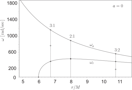
Figure 1: Resonance conditions in Schwarzschild spacetime (from Török & al., 2005)

It is well known that a parametric resonance occurs when

$$\omega_{r}=\frac{2\,\omega_{\theta}}{n},\quad n=1,2,3,{\rm...}$$ (47)

For black holes, $\omega_{\theta}>\omega_{r}$, and therefore the smallest value of $n$ consistent with the resonance is $n=3$ (Paper I), which corresponds to the $3/2$ ratio of the vertical and radial epicyclic frequencies. This is shown in Figure 1, along with a few other possible rational ratios of the vertical and radial epicyclic frequencies.

The radius (and frequency) at which the $3/2$ resonance occurs depends on the black hole spin $a$. Therefore, for sources with known mass, the observed QPO frequencies may be used for a direct measurement of the black hole spin, as was first done by Abramowicz & Kluźniak (2001).

Acknowledgments Most of the work reported here was supported by Nordita’s Nordic Project lead by M.A.A., and carried out at two Nordita workshops dedicated to the subject (with O.B. being an active participant in absentia). The paper was completed at the KITP, which is supported by the National Science Foundation under Grant No. PHY99-07949. W.K. was partially supported by KBN grant 2P03D01424.

References

References

- [1] [] Abramowicz M.A., 2005, Proceedings of the Nordita Workdays on QPOs, Astron. Nachr., 326
- [2] [] Abramowicz M.A., Jaroszyński M. & Sikora M., 1978, A&A, 63, 221
- [3] [] Abramowicz M.A. & Kluźniak W., 2001, A&A, 374, L19
- [4] [] Abramowicz M.A. & Kluźniak W., 2002, Gen. Relat. Grav., 35, 69
- [5] [] Biesiada M., 2003, Gen. Rel. Grav., 35, 1503
- [6] [] Blaes O.M., 1985, MNRAS, 216, 553
- [7] [] Blaes O.M., Abramowicz M.A., Kluźniak W. & Sramkova E., 2005, Paper III, in preparation
- [8] [] Colistete R.Jr., Leygnac C. & Kerner R. 2002, Class. Quant. Grav., 19, 4573
- [9] [] Kato S. & Fukue J., 1980, PASJ, 32, 377
- [10] [] Kerner R., van Holten J.W. & Colistete R.Jr., 2001, Class. Quant. Grav., 18, 4725
- [11] [] van der Klis M., 2000, Ann. Rev. Astr. Ap., 38, 717
- [12] [] van der Klis M., 2005, A review of rapid X-ray variability in X-ray binaries, astro-ph/0410551
- [13] [] Kluźniak W. & Abramowicz M.A., 2000, Phys. Rev. Lett., submitted, astro-ph/0105057
- [14] [] Kluźniak W. & Abramowicz M.A., 2001, Acta Phys. Pol. B, B32, 3605
- [15] [] Kluźniak W. & Abramowicz M.A., 2002, Paper I, A&A, submitted, astro-ph/0203314
- [16] [] Lee W.H., Abramowicz M.A. & Kluźniak W., 2004, ApJ, 603, L93
- [17] [] Madej J. & Paczyński B., 1977, IAU Colloq. 32, 313
- [18] [] McClintock J.E. & Remillard R.A., 2004, Black Hole Binaries astro-ph/0306213
- [19] [] Papaloizou J.C.B. & Pringle J.E., 1984, MNRAS, 208, 721
- [20] [] Remillard R.A., 2005, lectures given at the program “Physics of Astrophysical Outflows and Accretion Disks”, KITP University of California, Santa Barbara, June 2005
- [21] [] Remillard R.A., 2005, in Proceedings of the Nordita Workdays on QPOs, Astron. Nachr., ed. M.A. Abramowicz, 326 astro-ph/0510699
- [22] [] Silbergleit A.G., Wagoner R.V. & Ortega-Rodrígez M., 2001, ApJ, 548, 335
- [23] [] Synge J.L., 1960, Relativity: The general Theory, North-Holland, Amsterdam
- [24] [] Török G., Abramowicz M.A., Kluźniak W. & Stuchlík Z., 2005, A&A, 436, 1
- [25] [] Wald R.M, 1984, General Relativity, The University of Chicago Press, Chicago