Millihertz Quasi-Periodic Oscillations from Marginally Stable Nuclear Burning on an Accreting Neutron Star

Abstract

We investigate marginally stable nuclear burning on the surface of accreting neutron stars as an explanation for the mHz quasi-periodic oscillations (QPOs) observed from three low mass X-ray binaries. At the boundary between unstable and stable burning, the temperature dependence of the nuclear heating rate and cooling rate almost cancel. The result is an oscillatory mode of burning, with an oscillation period close to the geometric mean of the thermal and accretion timescales for the burning layer. We describe a simple one-zone model which illustrates this basic physics, and then present detailed multizone hydrodynamical calculations of nuclear burning close to the stability boundary using the Kepler code. Our models naturally explain the characteristic 2 minute period of the mHz QPOs, and why they are seen only in a very narrow range of X-ray luminosities. The oscillation period is sensitive to the accreted hydrogen fraction and the surface gravity, suggesting a new way to probe these parameters. A major puzzle is that the accretion rate at which the oscillations appear in the theoretical models is an order of magnitude larger than the rate implied by the X-ray luminosity when the mHz QPOs are seen. We discuss the implications for our general understanding of nuclear burning on accreting neutron stars. One possibility is that the accreted material covers only part of the neutron star surface at luminosities $L_{X}\gtrsim 10^{37}\ {\rm erg\ s^{-1}}$.

1. Introduction

Low mass X-ray binaries, in which a neutron star or black hole accretes from a low mass companion, exhibit a range of periodic and quasi-periodic phenomena, ranging in frequency from very low frequency (mHz) noise to kHz quasi-periodic oscillations (QPOs) (see van der Klis 2004 for a recent review). This variability has mostly been associated with orbiting material in the accretion flow close to the compact object. In the case of a neutron star accretor, an important question is whether any of these phenomena originate from or are associated with the neutron star surface. This is important for identifying the compact object as a neutron star or a black hole and offers a probe of the neutron star surface layers.

Unstable nuclear burning on neutron star surfaces has been studied for many years, and is observed as Type I X-ray bursts. The accreted hydrogen (H) and helium (He) fuel accumulates on the surface of the star and undergoes a thin shell instability, giving rise to a $10$–$100$ second burst of X-rays with typical energy $10^{39}$ ergs (for reviews, see Lewin, van Paradijs, & Taam 1993, 1995; Strohmayer & Bildsten 2003). Not all sources show Type I X-ray bursts, however, and in many sources the bursts are not frequent enough to burn all of the accreted fuel (van Paradijs, Penninx, & Lewin 1988; in ’t Zand et al. 2003). Bildsten (1993, 1995) suggested that a different mode of nuclear burning, involving slowly propagating fires over the neutron star surface, operates at high accretion rates, and manifests itself in the power spectrum of the source as very low frequency noise (VLFN). He found an anti-correlation between bursting and VLFN, supporting this picture.

Revnivtsev et al. (2001) discovered a new class of mHz QPOs in three Atoll sources, 4U 1608-52, 4U 1636-53, and Aql X-1, which they proposed were from a special mode of nuclear burning on the neutron star surface rather than from the accretion flow. These mHz QPOs have frequencies in the range $7$–$9\ {\rm mHz}$ (timescales of $1.9$–$2.4$ minutes). The associated flux variations are at the few per cent level, and are strongest at low photon energies ($\lesssim 5$ keV). This is in contrast to all other observed QPOs, whose amplitude generally increases with photon energy. Revnivtsev et al. (2001) showed that the centroid frequency of the mHz QPO was stable on year timescales in a given source, and the same to within tens of per cent in all three sources in which it was detected. In addition, the presence of the mHz QPOs is affected by Type I X-ray bursts: in 4U 1608-52, the mHz QPOs disappeared immediately following a Type I X-ray burst. In 4U 1608-52, a transient source whose luminosity is observed to change by orders of magnitude, the mHz QPO was only present within a narrow range of luminosity, $L_{X}\approx 0.5$–$1.5\times 10^{37}\ {\rm erg\ s^{-1}}$.

The association of the mHz QPOs with a surface phenomenon was strengthened by the results of Yu & van der Klis (2002), who showed that the kHz QPO frequency is anti-correlated with the luminosity variations during the mHz oscillation. This is opposite to the long term trend, which is that the kHz QPO frequency varies proportional to the X-ray luminosity, consistent with the inner edge of the accretion disk being pushed inwards at higher accretion rates. The anti-correlation observed by Yu & van der Klis (2002) during the mHz QPO cycle suggests that the inner edge of the disk moves outwards slightly as the luminosity increases during the cycle, perhaps consistent with enhanced radiation drag as the gas orbiting close to the neutron star is radiated by emission from the neutron star surface.

The fact that the properties of the mHz QPOs suggest that they are associated with the neutron star surface led Revnivtsev et al. (2001) to propose that a special mode of nuclear burning operates at luminosities $L_{X}\approx 0.5$–$1.5\times 10^{37}\ {\rm erg\ s^{-1}}$. The nature of the burning and the physics underlying the characteristic timescale of $\approx 2$ minutes, however, were unexplained. Bildsten (1993) gave the characteristic timescales of the burning layer that might be associated with sub-hertz phenomena. The thermal timescale of the layer is $t_{\rm therm}\approx 10$ s, the time to accrete the fuel is $t_{\rm accr}\approx 1000$ s at the Eddington accretion rate, and the time for a nuclear burning “fire” to propagate around the surface is estimated to be $\sim 10^{4}$ s. Bildsten (1993) proposed that if several fires are propagating around the star at a given time, the time-signature would be broad band noise with frequencies in the mHz range. None of the timescales he identified match the $\approx 2$ minute mHz QPO period, however.

The luminosity at which mHz QPOs are observed ($L_{X}\approx 10^{37}\ {\rm erg\ s^{-1}}$) is significant because it is similar to the luminosity at which a transition in burning behavior occurs, from frequent Type I X-ray bursting at low accretion rates to the disappearance of Type I X-ray bursts at high accretion rates. This transition is common to many X-ray bursters (e.g., Cornelisse et al. 2003), and is expected theoretically because at high accretion rates the fuel burns at a higher temperature, reducing the temperature-sensitivity of helium burning and quenching the thin shell instability. An outstanding puzzle is that theory predicts a transition accretion rate close to the Eddington rate (Bildsten 1998), which corresponds to luminosities $L_{X}\sim 10^{38}\ {\rm erg\ s^{-1}}$, much larger than observed. Paczynski (1983) pointed out that near the transition from instability to stability, oscillations are expected because the eigenvalues of the system are complex. Narayan & Heyl (2003) extended Paczynski’s one-zone analysis, calculating linear eigenmodes of truncated steady-state burning models. They too found complex eigenvalues near the stability boundary, and suggested that this might explain the mHz QPOs observed by Revnivtsev et al. (2001). The oscillation frequencies, however, were an order of magnitude too small.

In this paper, we show that the mHz QPO frequencies are, in fact, naturally explained as being due to marginally stable nuclear burning on the neutron star surface. At the boundary between unstable and stable burning, the temperature dependence of the nuclear heating rate and cooling rate almost cancel. The result is an oscillatory mode of burning, with an oscillation period close to the geometric mean of the thermal and accretion timescales for the burning layer, $(t_{\rm therm}t_{\rm accr})^{1/2}\approx 100\ {\rm s}$. In §2, we describe a simple one-zone model which illustrates this basic physics, and then present detailed hydrodynamical calculations of nuclear burning close to the stability boundary in §3. We discuss the implications of our results in §4. In particular, if the mHz QPOs are due to marginally stable nuclear burning, the local accretion rate onto the star must be close to the Eddington rate, even though the global accretion rate inferred from the X-ray luminosity is ten times lower.

2. A one-zone model

In this section, we discuss a simplified model of the burning layers which illustrates the basic physics underlying the oscillations observed in our multizone numerical simulations. Following Paczynski (1983), we consider a one-zone model of the burning layer. The temperature, $T$, and thickness of the fuel layer, $y$ (which we measure as a column depth, in units of mass per unit area), obey

$$c_{P}{dT\over dt} = \epsilon-{F\over y}$$ (1)

$${dy\over dt} = \dot{m}-{\epsilon\over E_{\star}}y.$$ (2)

(equivalent to eqns. [8] of Paczynski 1983). Equation (1) describes the heat balance, including heating of the layer by nuclear reactions $\epsilon$, and radiative cooling $-\mbox{\boldmath$\displaystyle\nabla$}\mbox{\boldmath$\displaystyle\cdot$}\,\mbox{\boldmath$\displaystyle F$}/\rho=dF/dy\approx F/y$. The heat capacity at constant pressure is $c_{P}$, and $F$ is the outwards heat flux. Equation (2) tracks the burning depth, allowing for accretion of new fuel at a rate given by the local accretion rate $\dot{m}$, as well as burning of fuel on a timescale $E_{\star}/\epsilon$, where $E_{\star}$ is the energy per gram released in the burning. Note that the pressure at the base of the layer is $P=gy$ from hydrostatic balance, where $g$ is the local gravity. We first study equations (1) and (2) analytically (§2.1), and then show some numerical integrations (§2.2).

2.1. Analytic estimates

Equations (1) and (2) constitute a nonlinear oscillator. To understand its behavior, we consider linear perturbations to the steady state solution, which has

$$\epsilon y=F=\dot{m}E_{\star}.$$ (3)

The nuclear energy generation is generally a strong function of temperature, and we will assume $\epsilon\propto T^{\alpha}$, where $\alpha\equiv d\ln\epsilon/d\ln T$. The heat flux is approximately $F\approx acT^{4}/3\kappa y$ (e.g., Bildsten 1998). To simplify the algebra in this section, we assume that $\epsilon$ depends only on temperature, and that the opacity $\kappa$ is a constant. We write the deviations from steady state as $\delta y$ and $\delta T$, giving

$$c_{P}{\partial\delta T\over\partial t} = \alpha\epsilon{\delta T\over T}-{4F\over y}{\delta T\over T}+{2F\over y}{\delta y\over y}$$ (4)

$${\partial\delta y\over\partial t} = -{\epsilon\over E_{\star}}\left(\delta y+{\alpha y\over T}\delta T\right).$$ (5)

Defining a thermal timescale for the layer $t_{\rm therm}=c_{p}T/\epsilon=c_{p}Ty/F$ and an accretion timescale $t_{\rm accr}=y/\dot{m}$, and using the steady-state relations of equation (3) gives

$${\partial\over\partial t}\left({\delta T\over T}\right) = \left({\alpha-4\over t_{\rm therm}}\right){\delta T\over T}+\left({2\over t_{\rm therm}}\right){\delta y\over y}$$ (6)

$${\partial\over\partial t}\left({\delta y\over y}\right) = -\left({1\over t_{\rm accr}}\right){\delta y\over y}-\left({\alpha\over t_{\rm accr}}\right){\delta T\over T}.$$ (7)

It is useful to write $\delta T=f(t)\exp(-t/t_{\rm accr})$ and $\delta y=g(t)\exp(-t/t_{\rm accr})$. This simplifies equations (6) and (7), allowing us to combine them into a single differential equation for $f$,

$${\partial^{2}f\over\partial t^{2}}+\left({4-\alpha\over t_{\rm therm}}-{1\over t_{\rm accr}}\right){\partial f\over\partial t}+{2\alpha\over t_{\rm accr}t_{\rm therm}}f=0.$$ (8)

Equation (8) is the equation for a damped simple harmonic oscillator. The solution is $\delta T\propto\exp(\lambda t)$, with

$$\lambda={1\over 2}\left({\alpha-4\over t_{\rm therm}}-{1\over t_{\rm accr}}\right)\pm\left[{1\over 4}\left({\alpha-4\over t_{\rm therm}}+{1\over t_{\rm accr}}\right)^{2}-{2\alpha\over t_{\rm therm}t_{\rm accr}}\right]^{1/2}.$$ (9)

Note that the “damping” term in equation (8) can be positive or negative depending on the relative temperature sensitivities of the heating and cooling.

Figure 1.— Lightcurves for the one-zone model at three different accretion rates. The system evolves from the arbitrary initial values $y=2\times 10^{8}\ {\rm g\ cm^{-2}}$ and $T=2\times 10^{8}\ {\rm K}$. At $\dot{m}=0.95\ \dot{m}_{\rm Edd}$, bursts occur with a recurrence time of 34 minutes. At $\dot{m}=0.998\ \dot{m}_{\rm Edd}$, oscillations are seen with a period of 4.7 minutes. At $\dot{m}=1.05\ \dot{m}_{\rm Edd}$, after a few transient oscillations, the burning evolves to a steady state. The steady state flux is $\dot{m}E_{\rm nuc}$, where $E_{\rm nuc}\approx 5$ MeV per nucleon.

Figure 2.— The trajectories in the temperature-column depth plane for the models shown in Figure 1. In each case, the model starts at the arbitrary point $y=2\times 10^{8}\ {\rm g\ cm^{-2}}$ and $T=2\times 10^{8}\ {\rm K}$.

The key to understanding the behavior of the burning is to note that the timescales $t_{\rm therm}$ and $t_{\rm accr}$ are very different. Steady burning at accretion rates near Eddington leads to ignition at a column depth $y\approx 10^{8}\ {\rm g\ cm^{-2}}$ and temperatures $T\approx 5\times 10^{8}\ {\rm K}$ (Schatz et al. 1999). The accretion timescale is therefore $y/\dot{m}\approx 1000\ {\rm s}$ for accretion at $\dot{m}\approx 10^{5}\ {\rm g\ cm^{-2}\ s^{-1}}$ (roughly the Eddington rate). For stable burning $F=\dot{m}E_{\star}$, giving $t_{\rm therm}=c_{P}Ty/F=(c_{P}T/E_{\star})(y/\dot{m})\approx 0.01\ t_{\rm accr}\approx 10\ {\rm s}$, since for an ideal gas, $c_{P}T\approx(5/2)(k_{B}T/m_{p})=7.2\ {\rm keV}\ T_{8}$ per nucleon, whereas $E_{\star}\approx 5\ {\rm MeV}$ per nucleon (Schatz et al. 1999).

Because $t_{\rm therm}\ll t_{\rm accr}$ the damping term is usually much larger than the oscillatory term, and the system is either positively or negatively overdamped depending on the sign of $(\alpha-4)$. When $\alpha>4$, the damping coefficient is negative, leading to strong exponential growth: the steady state solution is linearly unstable. When $\alpha<4$, the damping coefficient is positive, leading to strong damping: the steady-state solution is linearly stable. Close to marginal stability when $\alpha\approx 4$, however, the effective thermal timescale $t_{\rm therm}/\left|\alpha-4\right|$ becomes much longer than the accretion time, and the inequality is reversed, giving weakly damped or excited oscillations with oscillation frequency $\omega\approx(2\alpha/t_{\rm accr}t_{\rm therm})^{1/2}$. The condition to observe oscillations is that the oscillation frequency should be larger than the damping rate,

$$\left({2\alpha\over t_{\rm accr}t_{\rm therm}}\right)^{1/2}>{1\over 2}\left({\alpha-4\over t_{\rm therm}}+{1\over t_{\rm accr}}\right).$$ (10)

Note that this condition can be satisfied when $\lambda$ has either positive or negative real part, so that the oscillations may be excited or damped.

Neglecting the slight modification from the damping term, the oscillation period is $P_{\rm osc}=2\pi/\omega$, or

$$P_{\rm osc} \approx {2\pi\over(2\alpha)^{1/2}}\left({c_{P}T\over E_{\star}}\right)^{1/2}\left({y\over\dot{m}}\right)$$ (11)

$$= 3.1\ {\rm mins}\ \left({T_{8}\over 5}\right)^{1/2}y_{8}\left({\dot{m}\over\dot{m}_{\rm Edd}}\right)^{-1},$$

where we set $\alpha=4$ at marginal stability, and take $E_{\star}=5$ MeV per nucleon. This estimate is remarkably close to the observed mHz QPO period of $2$ minutes.

The physics of the oscillations can be understood by considering equations (6) and (7). For most accretion rates, the effective thermal time is much smaller than the accretion timescale, or $t_{\rm therm}/\left|4-\alpha\right|\ll t_{\rm accr}$. The perturbations are then effectively at constant pressure, or $\delta y=0$, as commonly assumed (see, e.g., Fujimoto, Hanawa, & Miyaji 1981; Bildsten 1998), and equation (6) leads directly to exponential growth or decay depending on the relative temperature sensitivities of the heating and cooling rates. Close to marginal stability, $(\alpha-4)\approx 0$, however, the effective thermal timescale becomes very long compared to the accretion time. Equations (6) and (7) in this limit are

$${\partial\over\partial t}\left({\delta T\over T}\right)\approx{2\over t_{\rm therm}}{\delta y\over y}$$ (12)

$${\partial\over\partial t}\left({\delta y\over y}\right)\approx-{\alpha\over t_{\rm accr}}{\delta T\over T}.$$ (13)

These equations nicely summarize the physics of the oscillations. Consider an upwards fluctuation in temperature $\delta T>0$. At the point of marginal stability, the increase in heating rate almost exactly cancels the $T^{4}$ dependence of the cooling rate. The main effect is that the hotter temperature leads to faster burning of the accreting fuel, and a decrease in thickness $\delta y<0$ on a timescale $\sim t_{\rm accr}$ (eq. [13]). But a thinner layer cools faster since $F/y\propto 1/y^{2}$. Therefore, the temperature fluctuation now begins to decrease, this time on the faster timescale $\sim t_{\rm therm}$ (eq. [12]). These changes are out phase, driving an oscillation on the intermediate timescale $\approx(t_{\rm therm}t_{\rm accr})^{1/2}$.

The behavior we describe here is shown by the canonical example of a nonlinear oscillator, the van der Pol oscillator (e.g., Abarbanel, Rabinovich, & Sushchik 1993). This oscillator consists of an LC circuit with an active element that can behave as a “negative resistor”, originally a vacuum tube. The governing equation is of the form $\ddot{x}+k(x^{2}-1)\dot{x}+\omega^{2}x=0$. Depending on the choice of control parameter $k$, the behavior of this circuit is a limit cycle (relaxation oscillations) with fast and slow timescales dominating at different parts of the cycle ($k>1$), a strongly damped system which evolves to a steady-state ($k<-1$), or oscillatory with growing or damped oscillations ($|k|<1$). These three states are analogous to bursting, stable burning, and oscillations near the stability boundary in the one-zone model.

2.2. Numerical integrations

We have integrated equations (1) and (2) in time to determine the non-linear evolution of the one-zone model. For the nuclear burning, we use the triple alpha reaction ($3\alpha\rightarrow^{12}$C) rate as given by Fushiki & Lamb (1987). We allow for the presence of hydrogen in the accreted fuel, however, by enhancing the energy release from the triple alpha reaction by a factor $E_{\rm nuc}/E_{3\alpha}$, where $E_{3\alpha}=0.606$ MeV per nucleon is the energy release from the triple alpha reaction, and $E_{\rm nuc}$ is the energy release from burning the accreted mixture of hydrogen and helium to iron group. We assume that $E_{\rm nuc}=1.6+4.9X_{0}$ MeV per nucleon, where $X_{0}$ is the mass fraction of hydrogen in the accreted layer. This expression for $E_{\rm nuc}$ includes an energy loss of 25% from neutrino emission during $\alpha$p- and rp-process burning (e.g., Fujimoto et al. 1987), and gives $E_{\rm nuc}=5$ MeV per nucleon for $X_{0}=0.7$, in good agreement with the energy release in the steady state burning models of Schatz et al. (1999). We write the flux as $F=acT^{4}/3\kappa y$ (Bildsten 1998), where the opacity $\kappa$ is calculated as described by Schatz et al. (1999). In addition, we include a flux heating the layer from below of 0.15 MeV per nucleon, and a contribution to the heating rate from hot CNO hydrogen burning in the accumulating fuel layer. Neither of these extra contributions to the heat balance make a significant difference to our results. Note that the amount of hydrogen burned by hot CNO cycle prior to helium ignition is very small at the rapid accretion rates considered here.

Figure 1 shows lightcurves from the one-zone integrations at different accretion rates. To enable a direct comparison with the multizone simulations discussed in §3, we set the local gravity to be the Newtonian gravity for a 1.4 $M_{\odot}$, 10 km neutron star, $g=1.9\times 10^{14}\ {\rm cm^{2}\ s^{-1}}$. Throughout this paper, we define the local Eddington accretion rate to be $\dot{m}_{\rm Edd}\equiv 8.8\times 10^{4}\ {\rm g\ cm^{-2}\ s^{-1}}$. By coincidence, the stability boundary for this one zone model is very close to the Eddington accretion rate. In Figure 1, we show lightcurves at $\dot{m}=0.95$, $0.998$, and $1.05\ \dot{m}_{\rm Edd}$. Figure 2 shows the corresponding tracks in the temperature-column depth plane. We start the simulations with the arbitrary conditions $T=2\times 10^{8}\ {\rm K}$, and $y=2\times 10^{8}\ {\rm g\ cm^{-2}}$. At accretion rates below the boundary, the system evolves quickly into a limit cycle corresponding to Type I X-ray bursts: slow accumulation of fuel followed by rapid burning. Close to the stability boundary, the recurrence time is $\approx 30$ minutes. At accretion rates above the boundary the evolution is to a steady state in which the fuel burns at $T\approx 5\times 10^{8}\ {\rm K}$ and $y\approx 7\times 10^{7}\ {\rm g\ cm^{-2}}$. For accretion rates very close to the transition, $\dot{m}\approx 1\ \dot{m}_{\rm Edd}$, we find oscillations around the steady state conditions, with oscillation period $\approx 4$ minutes and amplitude a few percent of the Eddington flux. For the oscillatory case, Figure 3 shows a more detailed view of the trajectory of the solution in the temperature-column depth phase space.

Figure 3.— The trajectory in the temperature-column depth plane for $\dot{m}=0.998\dot{m}_{\rm Edd}$, as shown in Figure 2, but zooming in on the oscillations around the steady burning location.

Figure 4.— Oscillation period as a function of accretion rate in the one-zone model, for different choices of surface gravity and accreted hydrogen fraction. At each accretion rate, we integrate the model for $10^{6}\ {\rm s}$, and plot the mean oscillation period, only including data for $t>100$ minutes. The solid symbols indicate models for which the oscillations grow and reach a steady amplitude; the open symbols indicate models for which the oscillations are damped.

Although the one-zone model is approximate, it is useful because it allows us to investigate how the properties of the oscillations change with parameters such as surface gravity and accreted composition. The accreted composition could differ from system to system either due to metallicity variations, or variations in the accreted hydrogen fraction. Intermediate-mass binary evolution models (e.g., Podsiadlowski et al. 2002) predict that the companion star in many systems is hydrogen deficient, so that the hydrogen mass fraction is reduced below the solar composition value of $X_{0}\approx 0.7$. The importance of the hydrogen fraction is that the nuclear energy release $E_{\rm nuc}$ changes significantly with only small changes in $X_{0}$. In contrast, we expect that metallicity will not have a large effect on the transition accretion rate or the oscillation period. This is because the metallicity of the accreted material mainly enters into the one-zone model as hot CNO hydrogen burning in the accumulating layer, but the flux from hot CNO burning, $\epsilon_{\rm CNO}y\approx 5\times 10^{21}\ {\rm erg\ cm^{-2}\ s^{-1}}\ y_{8}(Z_{\rm CNO}/0.01)$, is much smaller than the steady burning flux, $\dot{m}E_{\rm nuc}\approx 5\times 10^{23}\ {\rm erg\ cm^{-2}\ s^{-1}}\ (\dot{m}/\dot{m}_{\rm Edd})$, where $Z_{\rm CNO}$ is the mass fraction of CNO elements.

Figure 4 shows the dependence of the oscillation period on accretion rate for different choices of gravity and accreted hydrogen fraction. We show results for $g_{14}=1.9$, corresponding to the Newtonian gravity of a 1.4 $M_{\odot}$, 10 km neutron star (or the general relativistic gravity for a 1.4 $M_{\odot}$, 12.3 km neutron star), $g_{14}=2.45$, the gravity of a 1.4 $M_{\odot}$, 10 km neutron star taking general relativistic corrections into account, and a stronger gravity $g_{14}=3.1$ which corresponds to the general relativistic surface gravity for a $2\ M_{\odot}$, 11 km neutron star. We also show a model with a hydrogen fraction below solar, $X_{0}=0.5$. Only the accretion rate range at which oscillations are observed is shown. At each accretion rate, we integrate the one-zone model for $10^{6}$ seconds, and plot the mean oscillation period after discarding the first 100 minutes of data.

For each choice of $g_{14}$ and $X_{0}$, the pattern is similar. The overall range of accretion rates for which oscillations are seen is very narrow, $\Delta\dot{m}/\dot{m}\approx 1$%. For most of this range the oscillations are decaying. As the stability boundary is approached from below, we first see oscillations which reach a steady amplitude (indicated by solid squares in Fig. 4) whose frequency drops rapidly with increasing $\dot{m}$. At larger accretion rates (open squares in Fig. 4), the oscillations decay with time, on timescales $<1$ day, and have a frequency that is less sensitive to $\dot{m}$. The transition from growing to decaying oscillations is very rapid. In each case, the model indicated by the last closed square shows stable oscillations for $10^{6}$ seconds, whereas with only a small increment in accretion rate the next model (first open square) has oscillations which decay on a timescale of $\sim 10^{5}$ seconds. Most interesting is that the oscillation period is sensitive to $g_{14}$ and $X_{0}$. Increasing gravity or decreasing $X_{0}$ moves the transition from unstable to stable burning to higher accretion rates, where the oscillation period is shorter. As $X_{0}$ decreases, the accretion rate range over which the oscillations are growing rather than decaying is larger.

3. Multizone calculations of burning near the stability boundary

We now present detailed multi-zone models of nuclear burning at accretion rates close to the transition from unstable to stable burning. These models are extensions of the calculations presented by Woosley et al. (2004) using the implicit 1D hydrodynamic code Kepler (Weaver et al. 1978). Woosley et al. (2004) calculated sequences of X-ray bursts at accretion rates $\dot{M}\approx 0.03$ and $0.1\ \dot{M}_{\rm Edd}$. In this paper we show the first results of an extension of these calculations to higher accretion rates.

Following Woosley et al. (2004), we take the gravitational mass of the neutron star to be $1.4\ M_{\odot}$ and $R=10\ {\rm km}$, giving a Newtonian gravity $g_{14}=1.9$. The effects of general relativity are not included in the simulations itself, but because the burning layer is very thin the effects of general relativity are small over the extent of the simulated burning layer and a local Newtonian frame is a good approximation. General relativity may be accounted for using appropriate redshift factors, as discussed in §4.4 of Woosley et al. (2004). The results we provide here do not include these redshift corrections; the simulated conditions apply for different combinations of neutron star radius and mass that give the same surface acceleration in the local frame, using appropriate scaling of surface area, accretion rate, and luminosity.

Our code includes an adaptive nuclear reaction network that automatically adjusts to include or remove isotopes as needed to follow the details of the nucleosynthesis, out of a reaction rate library of about 5,000 nuclei (Rauscher et al. 2002). The calculations presented here use up to 1300 different isotopes. The reaction rate library includes recent measurements and estimates of critical nuclear reaction rates. The effect of uncertainties in these rates are discussed in detail in Woosley et al. (2004). The energy generation from the reaction network is directly and consistently coupled into the implicit hydrodynamic solver. The numerical grid adaptively refines and derefines the Lagrangian grid to resolve gradients, but in the hydrogen-rich layer in effect is essentially at constant mass resolution, i.e., linear in column depth. Accretion is modeled by periodically adding an extra zone at the surface of the star (of column depth $\approx 1.6\times 10^{6}\ {\rm g\ cm^{-2}}$) (Woosley et al. 2004). We follow both the compositional and thermal profiles of the layer, including radiative and convective transport, with a time-dependent mixing length treatment for convection, semiconvection, and thermohaline convection.

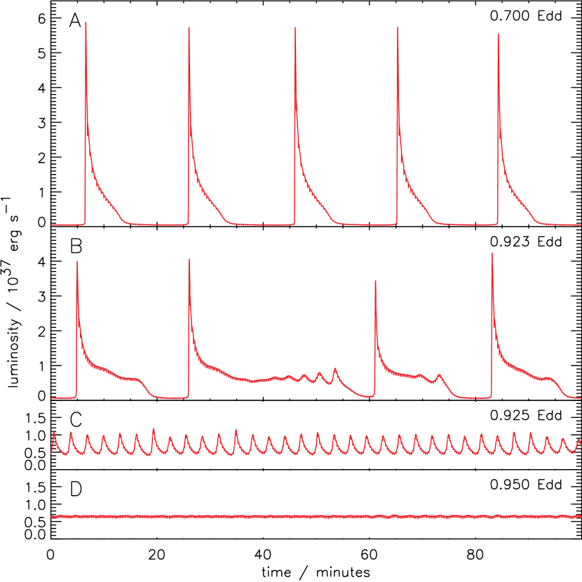
Figure 5.— Light curves for different accretion rates (the upper right corner gives accretion rate in units of Eddington accretion rate). Panel A shows regular bursting with stable recurrence times. Panel B shows weaker bursts with a partial oscillatory behavior in the tail of the burst light curves. Panel C shows oscillatory rather behavior and no bursts. Panel D shows very small oscillations, essentially stable behavior. The small dips seen in all lightcurves on about 15 s time-scale are an artifact of our treatment of accretion, in which an entire small outer zone is added periodically. The beginning of this figure is 10,000 s after the beginning of the simulation to allow the model to reach quasi-stationary conditions.

Here we present results for an accreted material metallicity of 1/20 solar. At an accretion rate $\dot{M}=0.1\ \dot{M}_{\rm Edd}$, Woosley et al. (2004) (their model zM) found a sequence of regular bursts with recurrence times close to 3 hours. Increasing the accretion rate in our new sequence of models, we find a transition from unstable to stable burning at $\dot{M}=0.924\ \dot{M}_{\rm Edd}$. Figure 5 shows the behavior close to the transition accretion rate. The lightcurves show a progression from regular periodic bursting at $\dot{M}=0.7\ \dot{M}_{\rm Edd}$ (with recurrence times close to $20$ minutes), to a combination of irregular bursts intermixed with oscillations at $\dot{M}=0.923\ \dot{M}_{\rm Edd}$, to a regular sequence of oscillations at $\dot{M}=0.925\ \dot{M}_{\rm Edd}$, and finally to stable burning at $\dot{M}=0.95\ \dot{M}_{\rm Edd}$, with the oscillation amplitude rapidly decreasing as the accretion rate is increased.

The oscillation period at $\dot{M}=0.923\ \dot{M}_{\rm Edd}$ is $185\pm 5$ seconds. Figure 6 shows a portion of the lightcurve at this accretion rate. The oscillations have an asymmetric profile, with the decay lasting twice as long as the rise. Revnitsev et al. (2001) noted marginal evidence that the peaks of the mHz QPOs were asymmetric, with a steep rise and shallower decline. A more detailed comparison of our models with observed lightcurves would be interesting, but clearly there should be significant harmonic components. The peak-to-peak amplitude of the oscillation in Figure 6 is $\approx 5\times 10^{36}\ {\rm erg\ s^{-1}}$, with minimum luminosity $\approx 5\times 10^{36}\ {\rm erg\ s^{-1}}$ and maximum luminosity $\approx 10^{37}\ {\rm erg\ s^{-1}}$. This is in good agreement with the one-zone model (compare the middle panel of Fig. 1; for a 10 km star, a flux of $\approx 10^{24}\ {\rm erg\ cm^{-2}\ s^{-1}}$ corresponds to a luminosity of $\approx 10^{37}\ {\rm erg\ s^{-1}}$).

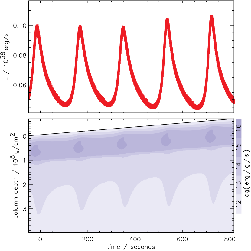
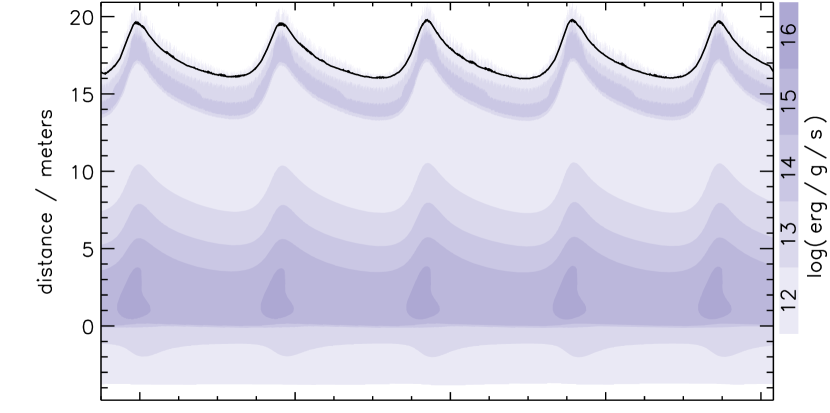
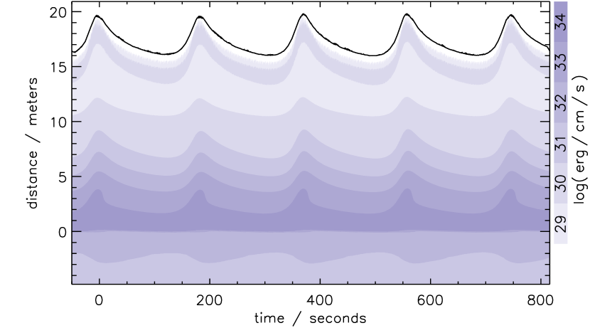
Figure 6.— Detailed light curve (upper panel) and specific nuclear energy generation as a function of time and column depth (lower panel). In the lower thee panels, each darker shading of blue corresponds to a value of energy generation one order of magnitude higher; see scale on right hand side of the figures. In the second figure from the top we label each depth with a Lagrangian column depth. Following a given column depth to the right shows the evolution of that fluid element in time. The sloping black line indicates the surface of the star (the slope gives the accretion rate). The lower two panels show the evolution s a function of radius coordinate. Zero is chosen to correspond to the location where hydrogen is depleted. The upper panel gives specific nuclear energy generation rate (same as the panel above), the bottom panel gives energy generation rate per unit depth.

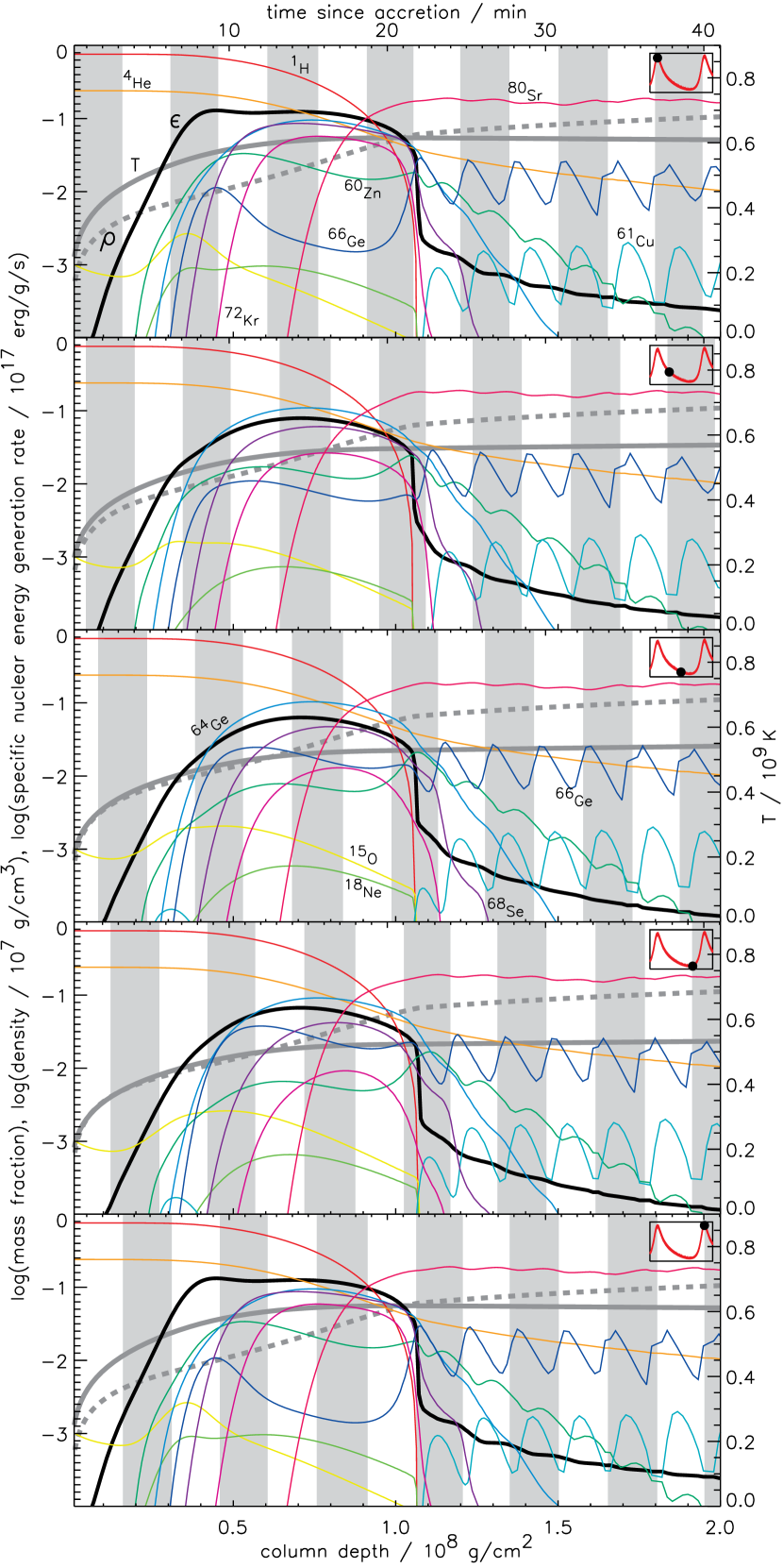
Figure 7.— Snapshots of structure (temperature: thick gray line; density: thick gray dashed line; specific nuclear energy generation: black line) and composition (select isotopes, colored lines) during one oscillation cycle; each panel is advanced in time by $P/4$ where $P$ is the oscillation period; the bottom panel is advanced by one full cycle. The bottom axis for each figure gives column depth, the top axis the corresponding time since accretion began. This is the same model as shown in Fig. 5, Panel C. The white and gray stripes correspond to one cycle of oscillation each, with the interfaces corresponding to the time of a maximum in the light curve at the time of the accretion of that layer. The small inserts at upper right corners indicate the position in the light curve (red) cycle of the snapshot (black dot; intentionally aligned with a layer interface). Note that the decreases of some of the radioactive isotopes in the right-hand side of the figure is due to their radioactive decay. An animation of this figure can be found at http://xrayburst.org/qpo.

Figure 8.— Variation of the composition (summed up for each mass number to be invariant against $\beta^{+}$ decays) in the ashes layer at a column depth close to $2\times 10^{8}\,$g cm^-2 (at the base of the composition profile shown in Fig. 7).

The nuclear burning in the oscillation mode is powered by $\alpha$p- and rp-process burning (Wallace & Woosley 1981; Schatz et al. 1999), beginning with seed nuclei produced by breakout reactions from the CNO cycle, and terminating at mass number $\approx 80$ (the most abundant nucleus is ⁸⁰Sr). Figure 6 shows the energy generation as a function of column depth, radius, and time through several oscillation cycles. Figure 7 shows the composition profile of the layer at different phases of the oscillation cycle. Beneath the hydrogen burning layer, the composition of the ashes shows periodic variations with a spacing in column depth of $\dot{m}P_{\rm osc}$, where $P_{\rm osc}=185$ seconds is the oscillation period. Note, however, that the hydrogen burning depth is relatively constant during the oscillation cycle. The hydrogen burns at a depth $\approx 10^{8}\ {\rm g\ cm^{-2}}$ which is $\approx 7$ times larger than the amount of mass accumulated in one oscillation cycle. The underlying ashes record the variations in burning temperature and the resulting variation of the rp-process ashes during the oscillation cycle. This is reminiscent of the growth of annual rings in a tree trunk. Figure 8 shows the distribution of nuclei in the ashes by mass number, and the slight variation in the composition through the cycle.

At the peak in the oscillation light curve, the increased temperature in the burning region drives heat transport inwards, heating the underlying material. This is similar to the substrate heating during Type I X-ray bursts discussed by Woosley et al. (2004), and leads to increase of burning of the ⁴He remaining in the ashes layer by the triple-$\alpha$ process and by $\alpha$ captures. In Figure 6 this can be seen as additional spikes in nuclear energy generation below the main burning band of the hydrogen-rich zone. Of particular interest is the amount of carbon remaining in the ashes. Stable burning of accreted H/He has been suggested as the source of carbon fuel for superbursts (in ’t Zand et al. 2003; Schatz et al. 2003). Figure 8 shows that the amount of carbon at $y\approx 2\times 10^{8}\ {\rm g\ cm^{-2}}$ is $\approx 2$ % by mass, which is very close to the asymptotic value of slightly below $2$ % in the deeper layers where all the helium has been burnt.

The layering of different compositions in the ashes does not persist to great depths. The different layers have different values of the number of electrons per baryon $Y_{\mathrm{e}}$, which determines the specific weight of fluid elements under the degenerate conditions in the ashes layer. The variation in composition is stable to the Rayleigh-Taylor instability because of the thermal buoyancy. Secular doubly-diffusive instabilities, however, cannot be suppressed. We find that the thermohaline or salt-finger instability grows in the layers which have an outwardly-decreasing $Y_{e}$ profile. The subsequent mixing is apparent in Figure 7 as the “erosion” of the peaks in the ⁶⁸Ge profile and the valleys of the ⁶¹Cu profiles at column depths above 1.5$\times 10^{8}\,$g cm². The mixing eventually leads to homogenization of the ashes layer at depths $>3\times 10^{8}\ {\rm g\ cm^{-2}}$. Our calculations followed that process to a point where the typical column-depth scale of the homogenized regions was several times that of the composition oscillations made by the oscillations in the burning region.

Schatz et al. (1999) calculated the nucleosynthesis in steady-state burning models at $\dot{m}=1\ \dot{m}_{\rm Edd}$. They found that the rp-process endpoint terminated at $A\approx 70$, and the carbon mass fraction was $\approx 5$%. We find slightly heavier rp-process ashes ($A\approx 80$), and a smaller carbon mass fraction ($\approx 2$%). This is consistent with the general anti-correlation found by Schatz et al. (2003) between the mass of nuclei produced in the rp-process and the carbon yield. In our case, a longer rp-process gives more time for helium to burn before the hydrogen runs out, leading to less carbon production following hydrogen exhaustion. Our burning temperature is approximately 10–20% hotter than the models of Schatz et al. (1999) which might explain the more extensive rp-process. This is perhaps because of a difference in radiative opacities: Schatz et al. (1999) use a fit to the results of Itoh et al. (1991) for free-free opacity, whereas the Kepler code uses the fit of Iben (1975) to the radiative opacities of Cox & Stewart (1970a,b). We will investigate this difference further in future calculations.

4. Discussion

The fact that oscillatory burning is naturally expected at the transition from unstable to stable nuclear burning was pointed out by Paczynski (1981). We have investigated the properties of marginally stable burning in this paper with a simplified one-zone model (§2) and with detailed multizone simulations (§3) using the Kepler code, extending the Type I X-ray burst calculations of Woosley et al. (2004) to higher accretion rates. The period, amplitude, and shape of the oscillations agree well in both models. Remarkably, the basic physics of the oscillations is the same physics underlying a nonlinear relaxation oscillator such as the van der Pol oscillator (e.g., Abarbanel et al. 1993). Usually, the positive or negative damping term dominates, giving rise to the familiar X-ray bursts at low accretion rates or stable burning at a fixed temperature and density at high accretion rates. Close to the marginally stable point, however, the effective thermal timescale is very long, allowing the underlying oscillation period of the system to be seen. This period is close to the geometric mean of the thermal time and accumulation time of the burning layer (eq. 11).

Figure 9.— Oscillation frequency as a function of hydrogen mass fraction, $X_{0}$, for different surface gravities, corresponding to different radii and masses of the underlying neutron star. The data is taken from one-zone models and rescaled to the oscillation frequency found in the multi-zone model with $X_{0}=0.7$ and $g_{14}=1.9$. Proper general relativistic redshifts corrections and radii have been applied. The curve for $g_{14}=0.9$ corresponds to $M=1.4\,M_{\odot}$ (gravitational mass) and $R=15.2\,$km, the curve for $g_{14}=1.48$ corresponds to $M=1.4\,M_{\odot}$ and $R=11.9\,$km, $g_{14}=1.9$ (used in the multi-zone calculation) corresponds to $M=1.4\,M_{\odot}$ and $R=12.3\,$km, the curve for $g_{14}=2.45$ is for $M=1.4\,M_{\odot}$ and $R=10\,$km, and the curve for $g_{14}=3.1$ corresponds to $M=2\,M_{\odot}$ and $R=11\,$km. The dotted lines indicate the boundaries of the observed range of QPO frequencies.

This behavior naturally reproduces two properties of the mHz QPOs observed by Revnivtsev et al. (2001): the observed periods of $\approx 2$ minutes, and the fact that mHz QPOs were observed in only a narrow range of luminosities in 4U 1608-52, $(0.5$–$1.5)\times 10^{37}\ {\rm erg\ s^{-1}}$. Identification of the mHz QPOs with marginally stable nuclear burning would for the first time relate a feature of the persistent X-ray emission to the neutron star surface in sources which are not X-ray pulsars. Further, our one-zone models indicate that the oscillation period is very sensitive to the surface gravity and accreted hydrogen fraction (Fig. 4). One of the difficulties in comparing X-ray burst properties with theoretical models is the uncertain relation between X-ray luminosity and accretion rate (e.g., Cumming 2003). This uncertainty is removed for marginally stable burning because it occurs at a specific accretion rate. The dependencies on surface gravity and hydrogen fraction need to be confirmed with multizone models, although unfortunately scanning the parameter space for the location of the transition is computationally very expensive. Our one-zone model results (Fig. 4) suggest that the observed periods of $\approx 2$ minutes require either $X_{0}<0.7$, as predicted by intermediate mass evolution models (e.g., Podsiadlowski et al. 2002), or surface gravity $g_{14}\approx 3$, for example corresponding to a $2\ M_{\odot}$ (gravitational mass) star with $R=11\ {\rm km}$. This can be seen in Figure 9, which shows the oscillation period as a function of $X_{0}$ and $g_{14}$. In this figure, we have rescaled the one-zone model results to match the multizone model for $X_{0}=0.7$ and $g_{14}=1.9$; in addition, we include the gravitational redshift factor. Future comparisons of theoretical models with mHz QPO periods and lightcurves are potentially sensitive probes of the surface gravity and accreted composition.

Two observed features of mHz QPOs remain to be explained. The first is the $Q$ value of the oscillation, which Revnivtsev et al. 2001 found to be $Q\equiv\nu/\Delta\nu\approx 3$–$4$. This may be related to the range of accretion rates for which oscillatory nuclear burning can be observed. Revnivtsev et al. (2001) constrained the range of luminosities at which mHz QPOs are present to be $(0.5$–$1.5)\times 10^{37}\ {\rm erg\ s^{-1}}$ in 4U 1608-52. In contrast, the theoretical range where oscillations are seen is much smaller, within a range $\Delta\dot{m}/\dot{m}\approx 0.01$ around the transition accretion rate. Moreover, for much of this range, the oscillations decay in time. Further observations which constrain the range of luminosities for which mHz QPOs can be observed would be valuable.

The second puzzle is that our theoretical models, in agreement with previous estimates (Fujimoto, Hanawa, & Miyaji 1981; Ayasli & Joss 1982; Bildsten 1998), find that the transition to stable burning occurs at an accretion rate close to the Eddington rate ($\dot{M}=0.924\ \dot{M}_{\rm Edd}$ for the model presented in §3). In contrast, the X-ray luminosity at which the mHz QPOs are observed in 4U 1608-52 is $\approx 0.5$–$1.5\times 10^{37}\ {\rm erg\ s^{-1}}$, implying an accretion rate ten times lower, $\dot{M}\approx 0.1\ \dot{M}_{\rm Edd}$. The same factor of ten appears when comparing the theoretical and observed oscillation amplitudes. The observed amplitudes of mHz QPOs correspond to flux variations of $\approx 1$–$2$% (Revnivtsev et al. 2001). As noted by Revnivtsev et al. (2001), this is consistent with the ratio of nuclear energy release from burning the accreted material to gravitational energy release from accretion. We find fractional amplitudes of the expected few percent level in the theoretical models. The absolute peak-to-peak flux variation is a factor of ten larger than observed, however, roughly $5\times 10^{23}\ {\rm erg\ cm^{-2}\ s^{-1}}$ or $5\times 10^{36}\ {\rm erg\ s^{-1}}$. This is more than $30$% of the observed persistent luminosity. Note that the oscillation amplitude decreases rapidly with increasing accretion rate above the transition accretion rate, so there does exist a small range of accretion rates where the amplitude does match the observed value.

A simple explanation for both of these discrepancies is that the local accretion rate onto the star is close to the Eddington rate, even though the global accretion rate is much lower. Because the burning layer is very thin, the properties of the burning depend only on the local accretion rate, which may vary across the surface of the star. In particular, if the accreted material spread over only $\approx 10$% of the surface, the local accretion rate would be ten times larger, comparable to the Eddington rate, and the emitted luminosity would be ten times lower than if the burning covered the entire stellar surface. This would allow marginally stable burning to occur at a global rate of $\approx 0.1$ Eddington, while giving flux variations of a few percent as observed.

The physics that might cause confinement of the fuel onto a small fraction of the surface is not obvious. The pressure at the base of the burning layer is $P=gy=10^{22}\ {\rm erg\ cm^{-3}}\ g_{14}y_{8}$, implying that magnetic fields of strength approaching $\approx\sqrt{8\pi P}\approx 3\times 10^{11}\ {\rm G}$ would be required to confine the fuel. This is much larger than the $\approx 10^{8}$–$10^{9}\ {\rm G}$ fields assumed for the neutron stars in LMXBs (believed to be the progenitors of the millisecond radio pulsars; Bhattacharya et al. 1995), although small scale fields of these strengths might exist on the surface. The need to transport angular momentum could also potentially delay spreading of material accreted from a disk onto the equator of the star. Inogamov & Sunyaev (1999) studied this problem with a one-zone model of the spreading layer and a basic prescription for angular momentum transport. They found column depths $<10^{4}\ {\rm g\ cm^{-2}}$ in the spreading layer, much smaller than the burning depth.

The possibility that the covering fraction changes with accretion rate was suggested previously by Bildsten (2000), but in the opposite sense, with covering fraction increasing with $\dot{m}$. The motivation was to explain a puzzling change in burst behavior that is observed to occur at a luminosity $\sim 10^{37}\ {\rm erg\ s^{-1}}$. EXOSAT observations of several Atoll sources showed that as X-ray luminosity increased, burst properties changed from regular, frequent bursts ($t_{\rm recur}\approx$ hours) with energetics consistent with burning all of the accreted fuel in bursts, to irregular, infrequent ($t_{\rm recur}>1$ day) bursts whose energetics indicate that only a small fraction of the fuel burns in bursts (van Paradijs et al. 1988). RXTE and BeppoSAX observations confirmed this result, with particularly good coverage for the transient source KS 1731-260 (Muno et al. 2000; Cornelisse et al. 2003). Cornelisse et al. (2003) found that observations of nine bursters with BeppoSAX were consistent with this pattern of bursting, with a universal transition luminosity $L_{X}\approx 2\times 10^{37}\ {\rm erg\ s^{-1}}$.

This change in bursting behavior is not predicted by the standard theory, in which regular bursting should continue up to the stability boundary at $\dot{m}\approx\dot{m}_{\rm Edd}$. Several theoretical explanations for the discrepancy were put forward, including mixing by Rayleigh-Taylor (Wallace & Woosley 1984) or shear instabilities (Fujimoto et al. 1987) which might allow more rapid burning of hydrogen, a new mode of burning involving slowly propagating fires at $\dot{m}\gtrsim 0.1\ \dot{m}_{\rm Edd}$ (Bildsten 1993), or that the covering fraction of accreted material increases at higher accretion rates, lowering the accretion rate per unit area and lengthening the time between bursts, giving hydrogen time to burn stably (Bildsten 2000). We also mention here that Narayan & Heyl (2003) calculated linear eigenmodes of truncated steady-state burning models, and found stability for accretion rates $\dot{M}>0.25\ \dot{M}_{\rm Edd}$, more consistent with observations. The lower accretion rate is likely the cause of the small oscillation frequencies that they found for marginally stable burning (period $\sim 20$ minutes). We find, however, that bursting continues unabated up to $\dot{M}\approx\dot{M}_{\rm Edd}$. Further work comparing linear stability analysis with numerical calculations seems to be required.

The observations of mHz QPOs at a luminosity close to $\approx 10^{37}\ {\rm erg\ s^{-1}}$ and their interpretation as marginally stable oscillatory burning at a local accretion rate $\dot{m}\approx\dot{m}_{\rm Edd}$ provide new input for these ideas. As we have discussed, if changes in the covering fraction are responsible, this suggests that the covering fraction decreases rather than increases at this luminosity. The observed Type I bursts at $L_{X}>10^{37}\ {\rm erg\ s^{-1}}$ could be accommodated if there was a slow “leak” of fuel away from the stably burning region. This fuel would deplete hydrogen as it accumulated, giving occasional short helium-rich bursts. Other mechanisms, such as stable burning driven by mixing of fuel by shear instabilities might also lead to oscillatory burning. More theoretical work is needed. One clue is that the ultracompact source 4U 1820-30 which most likely accretes pure helium (Bildsten 1995; Cumming 2003) shows a similar transition at a similar luminosity, implying that the nature of the transition does not depend on accreted composition.

This question is also likely to be relevant for superbursts and Type I burst oscillations. Superbursts are long duration, rare, and extremely energetic Type I X-ray bursts (up to 1000 times the duration and energy and less frequent than normal bursts) believed to be due to unstable carbon ignition (Cumming & Bildsten 2001; Strohmayer & Brown 2002). Superbursts are only observed at luminosities above $\approx 10^{37}\ {\rm erg\ s^{-1}}$, and from sources for which burst energetics indicate that bursts burn only a small fraction of the accreted fuel (in ’t Zand et al. 2003). This fits nicely with the theoretical result that stable burning is much more efficient than unstable burning at producing the carbon fuel (Schatz et al. 2003). How to achieve stable burning theoretically at $\dot{m}<\dot{m}_{\rm Edd}$, however, has been an open question. Type I burst oscillations are high frequency oscillations during Type I X-ray bursts believed to be due to burning asymmetries on the surface. Burst oscillations are preferentially seen at higher accretion rates, in the banana branch of the color-color diagram (e.g., Muno et al. 2000). Incomplete covering of the surface might help to explain the origin of burst oscillations, facilitating inhomogeneous burning when Type I X-ray bursts are able to occur.

Finally, we note that Atoll sources undergo a transition from the island state to banana branch in the color-color diagram at a luminosity of $L_{X}\approx 10^{37}\ {\rm erg\ s^{-1}}$. It is well-known for these sources that X-ray luminosity does not track accretion rate on short timescales (van der Klis 2001). One explanation for the transition from island state to banana branch in Atolls is that a hot quasi-spherical accretion flow at low rates is replaced by a thin disk at high rates (e.g., Gierlinski & Done 2002). If this picture is correct, it could be that the change in accretion geometry affects the distribution of fuel on the neutron star surface. An interesting observational question is whether the appearance of the mHz QPOs is linked to a particular luminosity range, or a particular part of the color-color diagram, for example the island to banana transition.

References

- (1) Abarbanel, H. D. I., Rabinovich, M. I., & Sushchik, M. M. 1993, “Introduction to Nonlinear Dynamics for Physicists” (Singapore: World Scientific)
- (2) Ayasli, S., & Joss, P. C. 1982, ApJ, 256, 637
- (3) Bildsten, L. 1993, ApJ, 418, L21
- (4) Bildsten, L. 1995, ApJ, 438, 852
- (5) Bildsten, L. 1998, NATO ASIC Proc. 515: The Many Faces of Neutron Stars., 419
- (6) Bildsten, L. 2000, American Institute of Physics Conference Series, 522, 359
- (7) Cornelisse, R., et al. 2003, A&A, 405, 1033
- (8) Cox, A. N., & Stewart, J. N. 1970, ApJS, 19, 243
- (9) Cox, A. N., & Stewart, J. N. 1970, ApJS, 19, 261
- (10) Cumming, A. 2003, ApJ, 595, 1077
- (11) Cumming, A. 2004, Nuclear Physics B Proceedings Supplements, 132, 435
- (12) Cumming, A., & Bildsten, L. 2001, ApJ, 559, L127
- (13) Fujimoto, M. Y., Hanawa, T., & Miyaji, S. 1981, ApJ, 247, 267
- (14) Fujimoto, M. Y., Sztajno, M., Lewin, W. H. G., & van Paradijs, J. 1987, ApJ, 319, 902
- (15) Fushiki, I., & Lamb, D. Q. 1987, ApJ, 317, 368
- (16) Gierliński, M., & Done, C. 2002, MNRAS, 337, 1373
- (17) Iben, I. 1975, ApJ, 196, 525
- (18) in ’t Zand, J. J. M., Kuulkers, E., Verbunt, F., Heise, J., & Cornelisse, R. 2003, A&A, 411, L487
- (19) Inogamov, N. A., & Sunyaev, R. A. 1999, Astronomy Letters, 25, 269
- (20) Lewin, W. H. G., van Paradijs, J., & Taam, R. E. 1993, Space Science Reviews, 62, 223
- (21) Lewin, W. H. G., van Paradijs, J., & Taam, R. E. 1995, in X-Ray Binaries, ed. W. H. G. Lewin, J. van Paradijs, & E. P. J. van den Heuvel (Cambridge: CUP), 175
- (22) Muno, M. P., Fox, D. W., Morgan, E. H., & Bildsten, L. 2000, ApJ, 542, 1016
- (23) Narayan, R., & Heyl, J. S. 2003, ApJ, 599, 419
- (24) Paczynski, B. 1983, ApJ, 264, 282
- (25) Podsiadlowski, Ph., Rappaport, S., & Pfahl, E. D. 2002, ApJ, 565, 1107
- (26) Rauscher, T., Heger, A., Hoffman, R. D., Woosley, S. E. 2002, ApJ, 576, 323
- (27) Revnivtsev, M., Churazov, E., Gilfanov, M., & Sunyaev, R. 2001, A&A, 372, 138
- (28) Schatz, H., Bildsten, L., Cumming, A., & Wiescher, M. 1999, ApJ, 524, 1014
- (29) Schatz, H., Bildsten, L., Cumming, A., & Ouellette, M. 2003, Nucl. Phys. A, 718, 247
- (30) Strohmayer, T. E., & Bildsten, L. 2003, in “Compact Stellar X-Ray Sources”, eds. W.H.G. Lewin and M. van der Klis (Cambridge: Cambridge University Press) (astro-ph/0301544)
- (31) Strohmayer, T. E., & Brown, E. F. 2002, ApJ, 566, 1045
- (32) van der Klis, M. 2001, ApJ, 561, 943
- (33) van der Klis, M. 2004, in “Compact Stellar X-Ray Sources”, eds. W.H.G. Lewin and M. van der Klis (Cambridge: Cambridge University Press) (astro-ph/0410551)
- (34) van Paradijs, J., Penninx, W., & Lewin, W. H. G. 1988, MNRAS, 233, 437
- (35) Wallace, R. K., & Woosley, S. E. 1981, ApJS, 45, 389
- (36) Wallace, R. K., & Woosley, S. E. 1984, “High Energy Transients in Astrophysics”, 319
- (37) Weaver, T. A., Zimmerman, G. B., & Woosley, S. E. 1978, ApJ, 225, 1021
- (38) Woosley, S. E., et al. 2004, ApJS, 151, 75
- (39) Yu, W., & van der Klis, M. 2002, ApJ, 567, L67
- (40)