Spectrum of magnetohydrodynamic turbulence

Abstract

We propose a phenomenological theory of strong incompressible magnetohydrodynamic turbulence in the presence of a strong large-scale external magnetic field. We argue that in the inertial range of scales, magnetic-field and velocity-field fluctuations tend to align the directions of their polarizations. However, the perfect alignment cannot be reached, it is precluded by the presence of a constant energy flux over scales. As a consequence, the directions of fluid and magnetic-field fluctuations at each scale $\lambda$ become effectively aligned within the angle $\phi_{\lambda}\propto\lambda^{1/4}$, which leads to scale-dependent depletion of nonlinear interaction and to the field-perpendicular energy spectrum $E(k_{\perp})\propto k_{\perp}^{-3/2}$. Our results may be universal, i.e., independent of the external magnetic field, since small-scale fluctuations locally experience a strong field produced by large-scale eddies.

1. Introduction.— Magnetohydrodynamic (MHD) turbulence is pervasive in astrophysical systems, where ranges of scales available for plasma fluctuations span many orders of magnitude, and the fluctuations commonly possess power-law spectral distributions, e.g., (Biskamp, 2003). For example, the spectrum and structure of MHD fluctuations are relevant for the physics of solar wind, interstellar scintillation, cosmic-ray propagation in galaxies, and heat conduction in cooling flows in galaxy clusters.

The spectrum of MHD turbulence was first addressed by Iroshnikov (1963) and Kraichnan (1965), who proposed the physical framework for describing the turbulent energy cascade mediated by a guiding magnetic field. However, recent numerical and analytic works have challenged these standard results and revived substantial interest to the fundamentals of strong MHD turbulence (Goldreich & Sridhar, 1995; Cho & Vishniac, 2000; Biskamp & Müller, 2000; Milano, et al, 2001; Maron & Goldreich, 2001; Müller, Biskamp & Grappin, 2003; Müller & Grappin, 2005; Haugen, Brandenburg, & Dobler, ; Ng, et al, 2003; Galtier, Pouquet, & Mangeney, 2005). To formulate the problem and to set the notation, we first describe the Irosnikov-Kraichnan (Iroshnikov, 1963; Kraichnan, 1965) and Goldreich-Sridhar (Goldreich & Sridhar, 1995) theories, and point out some discrepancies of these theories with recent high-resolution numerical findings. Then, we propose a new model for MHD turbulence, which is free of such discrepancies, and which explains the results of numerical simulations (Maron & Goldreich, 2001; Müller, Biskamp & Grappin, 2003; Müller & Grappin, 2005; Haugen, Brandenburg, & Dobler, ).

Consider a conducting fluid stirred by a random force with the correlation length $\Lambda_{0}$. The system size is larger than $\Lambda_{0}$, and viscosity and resistivity of the fluid are very small. The goal is to find the stationary energy spectrum of the resulting turbulent fluctuations in the inertial interval of scales, $\lambda\ll\Lambda_{0}$. Let us split the magnetic field into two parts, ${\bf B}(x,t)={\bf B}_{0}+{\bf b}(x,t)$, where ${\bf B}_{0}=\langle{\bf B}\rangle$ is the system-size averaged magnetic field, and ${\bf b}(x,t)$ is the fluctuating part. The MHD equations describing the evolution of the magnetic field and of the fluid-velocity field ${\bf v}(x,t)$ can be represented in the so-called Elsässer variables, ${\bf z}={\bf v}-{\bf b}$, and ${\bf w}={\bf v}+{\bf b}$:

$$\partial_{t}{\bf z}+({\bf V}_{A}\cdot\nabla){\bf z}+({\bf w}\cdot\nabla){\bf z}=-\nabla P,$$ (1)

$$\partial_{t}{\bf w}-({\bf V}_{A}\cdot\nabla){\bf w}+({\bf z}\cdot\nabla){\bf w}=-\nabla P,$$ (2)

where ${\bf V}_{A}={\bf B}_{0}/\sqrt{4\pi\rho}$ is the Alfvén velocity, $\rho$ is the fluid density, $P$ is the pressure that is determined from the incompressibility condition, $\nabla\cdot{\bf z}=0$ or $\nabla\cdot{\bf w}=0$, and we omit the terms representing large-scale forcing and small viscosity and resistivity.

To present the standard arguments of Iroshnikov and Kraichnan, let us note that owing to the symmetric form of system (1, 2) two classes of exact solutions exist. For ${\bf w}\equiv 0$, any function ${\bf z}={\bf g}({\bf r}-{\bf V}_{A}t)$ is the solution of the system; analogously, for ${\bf z}\equiv 0$, the solution is given by an arbitrary function ${\bf w}={\bf h}({\bf r}+{\bf V}_{A}t)$. From the form of the nonlinear terms in system (1, 2), one observes that Alfvén-wave packets, or “eddies,” propagating in the same direction along ${\bf B}_{0}$ do not interact. One has therefore to investigate interactions or eddies propagating in opposite directions.

Consider a wave packet of size $\lambda$ propagating along the large-scale field ${\bf B}_{0}$. We denote the corresponding perturbations (i.e., typical variations across the eddy) of the velocity and magnetic fields by $\delta v_{\lambda}$ and $\delta b_{\lambda}$; in the Alfvén wave, $\delta v_{\lambda}\sim\delta b_{\lambda}$. Its interaction with the counter propagating packet of the same size occurs during time $\lambda/V_{A}$. As follows from (1,2), during one interaction the eddies are deformed only slightly, $\Delta\delta v_{\lambda}\sim(\delta v_{\lambda}^{2}/\lambda)(\lambda/V_{A})$. Since different eddies are not correlated, the perturbations add up randomly, so the eddy is deformed considerably only after a large number of interactions, $N\sim(\delta v/\Delta\delta v_{\lambda})^{2}$. The time of energy transfer to a smaller eddy can thus be estimated as $\tau_{IK}(\lambda)\sim N\lambda/V_{A}\sim\lambda/\delta v_{\lambda}(V_{A}/\delta v_{\lambda}).$ This time is larger than the Kolmogorov dynamic time, $\tau(\lambda)\sim\lambda/\delta v_{\lambda}$, by the Alfvén factor $V_{A}/\delta v_{\lambda}$. Assuming that the energy flux over scales is constant, $\delta v^{2}_{\lambda}/\tau_{IK}={\rm const}$, we obtain the Iroshnikov-Kraichnan energy spectrum,

$$E_{IK}(k)=\langle|\delta{\bf v}(k)|^{2}\rangle k^{2}\propto k^{-3/2}.$$ (3)

The essential assumption of the Iroshnikov-Kraichnan picture is that the eddy size is the same in the field-parallel and field-perpendicular directions. However, numerical and observational data accumulated for the last 30 years indicate that in MHD turbulence the energy transfer occurs predominantly in the field-perpendicular direction, e.g., (Milano, et al, 2001; Biskamp, 2003). This raises the question whether anisotropy is crucial for the energy cascade, and whether it changes the spectrum of turbulence.

An elegant treatment of anisotropic MHD turbulence was proposed by Goldreich & Sridhar (1995). They suggested that as the energy cascade proceeds to smaller scales, turbulent eddies progressively become elongated along the large-scale field. Their field-parallel and field-perpendicular scales are found from the so-called critical-balance condition. This condition follows from two different estimates that are equivalent in the Goldreich-Sridhar picture. First, the field-parallel scale of an eddy is found from formal balance of the linear and nonlinear terms in the MHD equations (1,2), $V_{A}/l\sim\delta v_{\lambda}/\lambda$. Second, the field-parallel scale of an eddy can be obtained from the requirement that the magnetic field-line displacement in the eddy, $\xi\sim\delta b_{\lambda}l/V_{A}$, be comparable with the field-perpendicular eddy size, $\lambda$. The shape of the turbulent eddy in the Goldreich-Sridhar theory is schematically presented in Fig. 1. As a result, two counter propagating eddies are deformed strongly during only one interaction, and the energy transfer time is given by the Alfvén crossing time, $\tau_{GS}\sim l/V_{A}\sim\lambda/\delta v_{\lambda}$. The Goldreich-Sridhar theory thus predicts that due to local anisotropy, the energy-transfer time is reduced to the Kolmogorov estimate. The field-perpendicular energy spectrum is obtained from the condition of constant energy flux, $\delta v_{\lambda}^{2}/\tau_{GS}={\rm const}$, which gives

$$E_{GS}(k_{\perp})=\langle|\delta{\bf v}(k_{\perp})|^{2}\rangle k_{\perp}\propto k_{\perp}^{-5/3},$$ (4)

where $\delta{\bf v}(k_{\perp})=\int\delta{\bf v}({\bf x_{\perp}})\exp(-i{\bf k}_{\perp}\cdot{\bf x}_{\perp})d^{2}{x}_{\perp}$.

Recent high-resolution numerical simulations of MHD turbulence in a strong external magnetic field indeed confirmed the elongation of turbulent fluctuations along the large-scale magnetic-field (Milano, et al, 2001; Cho & Vishniac, 2000; Maron & Goldreich, 2001; Müller, Biskamp & Grappin, 2003). However, the field-perpendicular energy spectrum was consistently found to be close to $E(k_{\perp})\propto k_{\perp}^{-3/2}$ (Maron & Goldreich, 2001; Müller, Biskamp & Grappin, 2003; Müller & Grappin, 2005; Haugen, Brandenburg, & Dobler, ). Obviously, such a spectrum combined with the anisotropy of fluctuations contradicts both the Iroshnikov-Kraichnan and the Goldreich-Sridhar phenomenologies. This controversy motivated our interest in the problem.

In this paper we argue that filament-like eddies are, in fact, non-realizable. We propose that the small-scale turbulent eddies spontaneously develop angular alignment of their magnetic-field and velocity-field polarizations, which leads to their local anisotropy in the field-perpendicular plane. This effect is similar to the dynamic alignment known in the case of decaying MHD turbulence, where magnetic and velocity fluctuations approach the configuration ${\bf v}(x)\equiv{\bf b}(x)$ or ${\bf v}(x)\equiv-{\bf b}(x)$, depending of the initial conditions (Dobrowolny, Mangeney, & Veltri, 1980; Grappin, et al, 1982; Pouquet, Frisch, & Meneguzzi, 1986). In the aligned state, the nonlinear interaction is zero, see Eqs. (1,2).

We propose that in the case of driven turbulence the tendency to dynamic alignment is preserved, however, the precise alignment cannot be reached. The reason is an energy cascade toward small scales, which should be maintained by nonlinear interaction. We thus argue that at each scale $\lambda$, the alignment of fluctuations should reach the maximal level consistent with a constant energy flux through this scale. We demonstrate that this is achieved when the velocity and magnetic-field fluctuations $\delta{\bf v}_{\lambda}$ and $\pm\delta{\bf b}_{\lambda}$ align their directions within the angle $\phi_{\lambda}\propto\lambda^{1/4}$. The dynamic alignment in driven turbulence thus becomes scale-dependent. Quite remarkably, this leads to the field-perpendicular energy spectrum $E(k_{\perp})\propto k_{\perp}^{-3/2}$, which explains the numerical observations and resolves the above mentioned controversy.

As another important result, in our theory small-scale eddies can be viewed as sheets or “ribbons”, stretched along the magnetic-field lines. This explains the well known numerical fact that the dissipative structures in MHD turbulence are micro current sheets rather than filaments, e.g., (Biskamp, 2003; Biskamp & Müller, 2000; Maron & Goldreich, 2001). In the next section we introduce our model of anisotropic MHD turbulence. Preliminary results on the dynamic alignment in driven MHD turbulence can be found in our earlier work (Boldyrev, 2005).

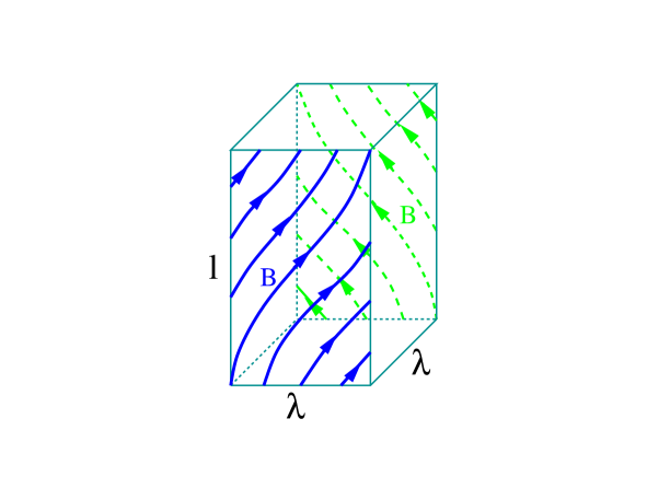
Figure 1: Sketch of a turbulent eddy in Goldreich-Sridhar picture. The large-scale magnetic field is in the vertical direction. The field perpendicular dimensions of the eddy are the same, while its field-parallel scale is $l\propto\lambda^{2/3}$. As the turbulent cascade proceeds toward the smallest, dissipative scales, $\lambda\to 0$, the Goldriech-Sridhar eddy assumes the shape of a filament.

2. Structure and spectrum of MHD turbulence.— As one can check, the MHD equations (1,2) conserve the integrals $\int z^{2}d^{3}x$ and $\int w^{2}d^{3}x$, if the fluctuations ${\bf w}(x)$ and ${\bf z}(x)$ have periodic boundary conditions or vanish at infinity. These integrals can be expressed through the integral of energy

$$E=\frac{1}{2}\int(b^{2}+v^{2})d^{3}x,$$ (5)

and the integral of cross-helicity,

$$H^{C}=\int({\bf v}\cdot{\bf b})d^{3}x.$$ (6)

In the unforced case, both integrals decay due to small viscosity and resistivity of the fluid. However, dissipation of cross-helicity is not sign-definite, and, therefore, the integral of cross-helicity decays slower than the integral of energy, e.g., (Biskamp, 2003). As a result of such “selective decay,” turbulence approaches the perfectly aligned configuration ${\bf b}(x)\equiv{\bf v}(x)$ or ${\bf b}(x)\equiv-{\bf v}(x)$ depending on the initial conditions. This behavior is known as the dynamic alignment or the Alfvénization effect (Dobrowolny, Mangeney, & Veltri, 1980; Grappin, et al, 1982; Pouquet, Frisch, & Meneguzzi, 1986). In the aligned state, either ${\bf z}(x)$ or ${\bf w}(x)$ is identically zero and nonlinear interaction vanishes.

We propose that a similar effect is present in driven MHD turbulence, since the external force locally produces large-scale fluctuations of cross-helicity, which are then inherited by smaller-scale eddies. Both $E$ and $H^{C}$ cascade toward small scales, however, the cascade rate of cross-helicity may generally be smaller than that of energy, which forces fluid and magnetic fluctuations to align their polarizations at each given scale. However, the precise alignment cannot be reached, it would be inconsistent with the constant energy flux over scales. Instead, the alignment of fluctuations should saturate at the maximal level that can be achieved in the presence of such a flux.

Let us first describe the shape of the eddy, which would be dictated solely by a constant energy flux, without any constraints imposed by the cross-helicity conservation (this derivation was first proposed in (Boldyrev, 2005)). Assume that directions of shear-Alfvén velocity- and magnetic-field fluctuations $\delta{\bf v}_{\lambda}$ and $\pm\delta{\bf b}_{\lambda}$ are aligned within some (small) angle $\theta_{\lambda}$ in the field-perpendicular plane. As one can directly check, this leads to depletion of the nonlinear interaction in Eqs. (1,2): $({\bf w}\cdot\nabla){\bf z}\sim({\bf z}\cdot\nabla){\bf w}\sim\theta_{\lambda}\delta v_{\lambda}^{2}/\lambda$. Similarly to the Goldreich-Sridhar critical balance, the eddy elongation in the field-parallel direction is found from balancing the linear and nonlinear terms in Eqs. (1,2), $l\sim V_{A}\lambda/(\delta v_{\lambda}\theta_{\lambda})$. The energy transfer time is then calculated as the Alfvén crossing time, $\tau_{N}\sim l/V_{A}\sim\lambda/(\delta v_{\lambda}\theta_{\lambda})$. It is important that such turbulence is strong and essentially three-dimensional.

To determine the shape of the eddy, we require that the energy flux be constant for all scales, $\delta v_{\lambda}^{2}/\tau_{N}={\rm const}$. This leads to the scaling of velocity fluctuations $\delta v_{\lambda}\propto(\lambda/\theta_{\lambda})^{1/3}$. The displacement of magnetic-field lines is given by $\xi\sim\delta v_{\lambda}l/V_{A}$, and the correlation length of fluctuations in the field-displacement direction cannot be smaller than $\xi$. Remarkably, the obtained shape of the eddy satisfies $\lambda/\xi\sim\theta_{\lambda}$, so it is indeed consistent with the assumed alignment of fluctuations within the angle $\theta_{\lambda}$. Note that in contrast with the Goldreich-Sridhar picture, in our model the eddy is three-dimensionally anisotropic, $l\gg\xi\gg\lambda$, see Fig. 2.

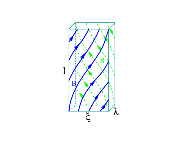
Figure 2: Anisotropic turbulent eddy in our picture. The large-scale magnetic field is in the vertical direction. The field-perpendicular dimensions of the eddy are $\lambda$ and $\xi\propto\lambda^{3/4}$, and the eddy size in the field-parallel direction is $l\propto\lambda^{1/2}$. As the energy cascade proceeds toward the smallest, dissipative scales, $\lambda\to 0$, the eddy assumes the shape of a current sheet.

It is natural to assume that turbulent fluctuations are scale invariant, which means that $\theta_{\lambda}$ is a power-law function of $\lambda$. We may parametrize $\theta_{\lambda}\propto\lambda^{\alpha/(3+\alpha)}$, which leads to $\delta v_{\lambda}\propto\lambda^{1/(3+\alpha)}$, $\xi\propto\lambda^{3/(3+\alpha)}$, $l\propto\lambda^{2/(3+\alpha)}$. We thus obtain that the sole requirement of constant energy flux does not define the eddy shape uniquely, but leads to a one-parameter family of solutions. The theory is self-consistent for an arbitrary parameter $\alpha\geq 0$. (Note that Goldreich-Sridhar model is a particular solution corresponding to $\alpha=0$.) In order to address the crucial question about the value of $\alpha$, we now have to use the second conserved quantity – cross-helicity. In other words, we want to find $\alpha$ that minimizes the total angular mismatch between the velocity and magnetic-field polarizations in the eddy.

The mismatch angle in the field-perpendicular (horizontal) plane is $\theta_{\lambda}\propto\lambda^{\alpha/(3+\alpha)}$. However, the polarization vectors are also mismatched in the vertical direction. To obtain the vertical alignment angle, ${\tilde{\theta}}_{\lambda}$, we note that in the regime of strong turbulence, eddies propagating along a large-scale magnetic field interact efficiently during only one crossing time. Therefore, only the local direction of the magnetic field matters, and when we speak about eddy elongation in the field-parallel direction, $l$, we should mean the eddy dimension along the local magnetic field (this was established by Cho & Vishniac (2000)). It is however important to note that the direction of the local magnetic field at the scale $\lambda$ cannot be defined precisely. Since the corresponding eddy contains magnetic field lines wandering within the angle ${\tilde{\theta}}_{\lambda}\sim\xi/l\propto\lambda^{1/(3+\alpha)}$, the direction of the local magnetic field can only be defined with the same accuracy. This means that the directions of shear-Alfvén velocity-field and magnetic-field fluctuations are aligned in the vertical direction within the angle ${\tilde{\theta}}_{\lambda}$, as is sketched in Fig. 3. Since both alignment angles, $\theta_{\lambda}$ and $\tilde{\theta}_{\lambda}$, are small, the total angular mismatch between $\delta{\bf v}_{\lambda}$ and $\pm\delta{\bf b}_{\lambda}$ can be calculated as $\phi_{\lambda}=\sqrt{\theta_{\lambda}^{2}+{\tilde{\theta}}_{\lambda}^{2}}$.

Following our strategy, we now require that the alignment angle $\phi_{\lambda}$ be minimal. We however observe that the obtained shape of the eddy precludes us from achieving the perfect alignment, $\phi_{\lambda}=0$. Indeed, if for a given small scale $\lambda$, we try to maximally align the polarizations in the field-perpendicular (horizontal) direction, i.e., to minimize $\theta_{\lambda}\propto\lambda^{\alpha/(3+\alpha)}$, we need to set $\alpha\to\infty$. In this case, the fluctuations will be completely misaligned in the vertical direction, ${\tilde{\theta}}\propto\lambda^{1/(3+\alpha)}\sim 1$. Similarly, if we try to maximally align them in the vertical direction, $\alpha\to 0$, they become misaligned in the horizontal plane. This “uncertainty” is minimized when $\theta_{\lambda}\sim{\tilde{\theta}}_{\lambda}$, in which case the maximal angular alignment is achieved and preserved for all scales. This determines the scaling parameter uniquely: $\alpha=1$. The resulting scaling of velocity fluctuations is $\delta v_{\lambda}\propto\lambda^{1/4}$, and the field-perpendicular energy spectrum has the form

$$E(k_{\perp})\propto k_{\perp}^{-3/2}.$$ (7)

The obtained structure and spectrum of turbulent fluctuations is the main result of this paper.

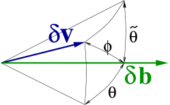
Figure 3: Sketch of three-dimensional angular alignment of shear-Alfvén velocity and magnetic-field fluctuations. The alignment angles consistent with an energy cascade are given by $\theta\propto\lambda^{\alpha/(3+\alpha)}$ and ${\tilde{\theta}}\propto\lambda^{1/(3+\alpha)}$. The maximal alignment is achieved for $\alpha=1$ (see the text).

3. Discussion and conclusion.— It may be reasonable to believe that an external magnetic field is not essential for our derivation. Indeed, a local guiding field for small-scale fluctuations is naturally provided by large-scale eddies, e.g., (Maron & Goldreich, 2001; Milano, et al, 2001). By this analogy, the spectrum of isotropic MHD turbulence should have scaling (7) as well. We however note that to observe this spectrum in numerical simulations of isotropic turbulence one would need to reach extremely high resolution (to ensure $\delta b_{\lambda}/\delta b_{\Lambda_{0}}\ll 1$), which is impossible with present-day computer power.

We also note that our theory naturally explains the presence of ribbon-like dissipative structures (current sheets) in numerical simulations of MHD turbulence (Biskamp & Müller, 2000; Maron & Goldreich, 2001). Indeed, the form of the eddy predicted in our model converges to such a structure as $\lambda\to 0$.

On the observational side, MHD turbulence is invoked to explain solar-wind measurements, e.g., (Goldsten, Roberts & Matthaeus, 1995) and interstellar scintillation, e.g., (Lithwick & Goldreich, 2001). Although the inferred spectra of magnetic-field and electron-density fluctuations are broadly consistent with the $-5/3$ scaling, there do exist indications in favour of “$-3/2$” in some diffractive scintillation (Shishov et al, 2003).

In conclusion, we propose that similarly to decaying MHD turbulence, driven MHD turbulence tends to align the polarizations of magnetic- and velocity-field fluctuations. However, the dynamic alignment cannot be perfect: perfectly aligned fluctuations do not interact and cannot carry energy flux. We therefore require that the alignment be maximal under the constraint of constant energy flux. Such requirement defines the alignment angle uniquely, $\phi_{\lambda}\propto\lambda^{1/4}$, which means that the strength of nonlinear interaction in driven MHD turbulence is reduced by the factor $\propto\lambda^{1/4}$ compared to a simple dimensional estimate $(\delta v_{\lambda})^{2}/\lambda$. The resulting fluctuations are three-dimensionally anisotropic (Fig. 2), and their energy spectrum is $E(k_{\perp})\propto k_{\perp}^{-3/2}$, in good agreement with numerical results.