Spectrophotometric properties of galaxies at intermediate redshifts (z~0.2–1.0)

We present the gas-phase oxygen abundance (O/H) for a sample of 131 star-forming galaxies at intermediate redshifts ($0.2<z<1.0$). The sample selection, the spectroscopic observations (mainly with VLT/FORS) and associated data reduction, the photometric properties, the emission-line measurements, and the spectral classification are fully described in a companion paper (Paper I). We use two methods to estimate the O/H abundance ratio: the “standard” $R_{\mathrm{23}}$ method which is based on empirical calibrations, and the CL01 method which is based on grids of photo-ionization models and on the fitting of emission lines. For most galaxies, we have been able to solve the problem of the metallicity degeneracy between the high- and low-metallicity branches of the O/H vs. $R_{\mathrm{23}}$ relationship using various secondary indicators. The luminosity – metallicity ($L-Z$) relation has been derived in the $B$- and $R$-bands, with metallicities derived with the two methods ($R_{\mathrm{23}}$ and CL01). In the analysis, we first consider our sample alone and then a larger one which includes other samples of intermediate-redshift galaxies drawn from the literature. The derived $L-Z$ relations at intermediate redshifts are very similar (same slope) to the $L-Z$ relation obtained for the local universe. Our sample alone only shows a small, not significant, evolution of the $L-Z$ relation with redshift up to $z\sim 1.0$. We only find statistical variations consistent with the uncertainty in the derived parameters. Including other samples of intermediate-redshift galaxies, we find however that galaxies at $z\sim 1$ appear to be metal-deficient by a factor of $\sim 3$ compared with galaxies in the local universe. For a given luminosity, they contain on average about one third of the metals locked in local galaxies.

1 Introduction

The understanding of galaxy formation and evolution has entered a new era since the advent of 10-m class telescopes and the associated powerful multi-object spectrograph, such as VIMOS on the VLT or DEIMOS on Keck. It is now possible to collect spectrophotometric data for large samples of galaxies at various redshifts, in order to compare the physical properties (star formation rate, extinction, metallicity, etc) of galaxies at different epochs of the Universe, using the results of recent surveys such as the “Sloan Digital Sky Survey” (SDSS, Abazajian et al. 2003, 2004 and the “2 degree Field Galaxy Redshift Survey” (2dFGRS, Colless et al. 2001) as references in the local Universe.

The correlation between galaxy metallicity and luminosity in the local universe is one of the most significant observational results in galaxy evolution studies. Lequeux et al. (1979) first revealed that the oxygen abundance O/H increases with the total mass of irregular galaxies. To avoid several problems in the estimate of dynamical masses of galaxies, especially for irregulars, absolute magnitudes are commonly used. The luminosity – metallicity ($L-Z$) relation for irregulars was later confirmed by Skillman, Kennicutt, & Hodge (1989), Richer & McCall (1995) and Pilyugin (2001) among others. Subsequent studies have extended the $L-Z$ relation to spiral galaxies (Garnett & Shields 1987; Zaritsky et al. 1994; Garnett et al. 1997; Pilyugin & Ferrini 2000), and to elliptical galaxies (Brodie & Huchra 1991). The luminosity correlates with metallicity over $\sim 10$ magnitudes in luminosity and 2 dex in metallicity, with indications that the relationship may be environmental- (Vilchez 1995) and morphology- (Mateo 1998) free. This suggests that similar phenomena govern the $L-Z$ over the whole Hubble sequence, from irregular/spirals to ellipticals (e.g. Garnett 2002; Pilyugin, Vílchez, & Contini 2004). Recently, the $L-Z$ relation in the local universe has been derived using the largest datasets available so far, namely the 2dFGRS (Lamareille et al. 2004) and the SDSS (Tremonti et al. 2004). The main goal of this paper is to derive the $L-Z$ relation for a sample of intermediate-redshift star-forming galaxies, and investigate how it compares with the local relation.

Recent studies of the $L-Z$ relation at intermediate redshifts have provided conflicting evidence for any change in the relation and no consensus has been reached. Kobulnicky & Zaritsky (1999) and Lilly, Carollo, & Stockton (2003) found their samples of intermediate-redshift galaxies to conform to the local $L-Z$ relation without any significant evolution of this relation out to $z\sim 1$. In contrast, other authors (e.g. Kobulnicky et al. 2003; Maier et al. 2004; Liang et al. 2004; Hammer et al. 2005; Kobulnicky & Kewley 2004) have recently claimed that both the slope and zero point of the $L-Z$ relation evolve with redshift, the slope becoming steeper and the zero point decreasing at early cosmic time. This would mean that galaxies of a given luminosity are more metal-poor at higher redshift, showing a decrease in average oxygen abundance by $\sim 0.15$ dex from $z=0$ to $z=1$.

In this paper, we present gas-phase oxygen abundance measurements for 131 star-forming galaxies in the redshift range $0.2<z<1.0$. The sample selection, the spectroscopic observations and data reduction, the photometric properties, the emission-line measurements, and the spectral classification of a sample of 141 intermediate-redshift emission-line galaxies are detailed in Lamareille et al. (2005), hereafter Paper I. Among the sample of 131 star-forming galaxies, 16 objects may contain a contribution from a low-luminosity active galactic nucleus and are thus flagged as “candidate” star-forming galaxies (see Paper I for details). Spectra were acquired mainly with the FORS1/2 (FOcal Reducer Spectrograph) instrument on the VLT, with the addition of LRIS (Low Resolution Imaging Spectrograph) observations on the Keck telescope, and galaxies selected from the “Gemini Deep Deep Survey” (GDDS, Abraham et al. 2004) public data release. The spectra are sorted into three sub-samples with different selection criteria: the “CFRS sub-sample” contains emission-line galaxies selected from the “Canada-France Redshift Survey” (Lilly et al. 1995), the “CLUST sub-sample” contains field galaxies randomly selected behind lensing clusters, and the “GDDS sub-sample” stands for galaxies taken from the GDDS survey.

These new data increase significantly the number of metallicity estimates available for this redshift range and are among the highest quality spectra yet available for the chemical analysis of intermediate-redshift galaxies. In addition to providing new constraints on the chemical enrichment of galaxies over the last $\sim 8$ Gyr, we hope that these measurements will be useful in modeling the evolution of galaxies on cosmological timescales. These new data are combined with existing emission-line measurements from the literature to assess the chemical evolution of star-forming galaxies out to $z=1$. In the near future, this work will be extended to samples of thousands of galaxies up to $z\sim 1.5$, thanks to the massive ongoing deep spectroscopic surveys such as the “VIMOS VLT Deep Survey” (VVDS, Le Fèvre et al. 2004).

The paper is organized as follows: Sect. 2 discusses the methods we have used to estimate the gas-phase oxygen abundance, and how we have addressed the issue of degeneracy in the determination of the oxygen abundance from strong emission lines. In Sect. 3 we study the relation between the luminosities and the metallicities of our sample galaxies, combined with other samples of intermediate-redshift galaxies published so far. Finally, in Sect. 3.4, we discuss the possible evolution of the $L-Z$ relation with redshift.

Throughout this paper, we use the WMAP cosmology (Spergel et al. 2003): $H_{\mathrm{0}}=71$ km s^-1 Mpc^-1, $\Omega_{\Lambda}=0.73$ and $\Omega_{\mathrm{\mathrm{m}}}=0.27$. The magnitudes are given in the AB system.

2 Gas-phase oxygen abundance

Emission lines are the primary source of information regarding gas-phase chemical abundances within star-forming regions. The “direct” method for determining the chemical composition requires the electron temperature and the density of the emitting gas (e.g. Osterbrock 1989). Unfortunately, a direct heavy-element abundance determination, based on measurements of the electron temperature and density, cannot be obtained for faint galaxies. The [Oiii]$\lambda$4363 auroral line, which is the most commonly applied temperature indicator in extragalactic Hii regions, is typically very weak and rapidly decreases in strength with increasing abundance; it is expected to be of order $10^{2}-10^{3}$ times fainter than the [Oiii]$\lambda$5007 line.

Given the absence of reliable [Oiii]$\lambda$4363 detections in our spectra of faint objects, alternative methods for deriving nebular abundances must be employed that rely on observations of the bright lines alone. Empirical methods to derive the oxygen abundance exploit the relationship between O/H and the intensity of the strong lines via the parameter $R_{\mathrm{23}}$=([Oiii]$\lambda\lambda$4959+5007+[Oii]$\lambda$3727)/H$\beta$ (see Fig. 1).

Many authors have developed techniques for converting $R_{\mathrm{23}}$ into oxygen abundance, both for the metal-poor (Pagel, Edmunds, & Smith 1980; Skillman 1989; Pilyugin 2000) and metal-rich (Pagel et al. 1979; Edmunds & Pagel 1984; McCall et al. 1985) regimes. On the upper, metal-rich branch of the $R_{\mathrm{23}}$ vs. O/H relationship, $R_{\mathrm{23}}$ increases as metallicity decreases via reduced cooling, elevated electronic temperatures, and a higher degree of collisional excitation. However, the relation between $R_{\mathrm{23}}$ and O/H becomes degenerate below 12+log(O/H)$\sim 8.4$ ($Z\sim 0.3\,Z_{\odot}$) and $R_{\mathrm{23}}$ reaches a maximum (see Fig. 1).

For oxygen abundances below 12+log(O/H)$\sim 8.2$, $R_{\mathrm{23}}$ decreases with decreasing O/H — this defines the lower, metal-poor branch. The decrease in $R_{\mathrm{23}}$ takes place because the greatly reduced oxygen abundance offsets the effect of reduced cooling and raised electron temperatures caused by the lower metal abundance. In this regime, the ionization parameter, defined by the emission-line ratio $O_{\mathrm{32}}$=[Oiii]$\lambda\lambda$4959+5007/[Oii]$\lambda$3727, also becomes important (McGaugh 1991).

The typical spread in the $R_{\mathrm{23}}$ vs. O/H relationship is $\pm 0.15$ dex, with a slightly larger spread ($\pm 0.25$ dex) in the turnaround region near 12+log(O/H)$\sim 8.4$. This dispersion reflects the uncertainties in the calibration of the $R_{\mathrm{23}}$ method which is based on photo-ionization models and observed Hii regions. However, the most significant uncertainty involves deciding whether an object lies on the upper, metal-rich branch, or on the lower, metal-poor branch of the curve (see Fig. 1).

In this paper, we use the strong-line method to estimate the gas-phase oxygen abundance of our sample galaxies using the emission line measurements reported in Paper I. Two different methods are considered: the $R_{\mathrm{23}}$ method (McGaugh 1991; Kewley & Dopita 2002) which is based on empirical calibrations between oxygen-to-hydrogen emission-line ratios and the gas-phase oxygen abundance, and the Charlot & Longhetti (2001, hereafter CL01) method which is based on the simultaneous fit of the luminosities of several emission lines using a large grid of photo-ionization models. The CL01 method has the potential of breaking the degeneracies in the determination of oxygen abundance (see CL01 for details), but we must point out that both the $R_{\mathrm{23}}$ estimator and the CL01 approach are limited by the O/H degeneracy when only a few emission lines are used, unless further information exists. However, the use of these two methods provides an important consistency check.

Figure 1: Calibration of gas-phase oxygen abundance as a function of the strong-line ratio log($R_{\mathrm{23}}$) (based on equivalent width measurements). Calibration curves from McGaugh (1991) (analytical formulae from Kobulnicky et al. 1999) are shown for three different values of the ionization parameter expressed in terms of the observable line ratio log($O_{\mathrm{32}}$) ($-$1, 0 and 1). Our sample of intermediate-redshift galaxies are plotted with the following symbols: filled circles are for “normal” objects, while the triangles represent intermediate-metallicity galaxies (see Sect. 2.1.2 for details).

2.1 The $R_{\mathrm{23}}$ method

We first discuss the commonly used $R_{\mathrm{23}}$ method which is based on empirical calibrations as mentioned above. This method uses two emission-line ratios: $R_{\mathrm{23}}$=([Oiii]$\lambda\lambda$4959+5007+[Oii]$\lambda$3727)/H$\beta$, and $O_{\mathrm{32}}$=[Oiii]$\lambda\lambda$4959+5007/[Oii]$\lambda$3727. Analytical expressions between the gas-phase oxygen-to-hydrogen abundance ratio and these two emission-line ratios are found in Kobulnicky, Kennicutt, & Pizagno (1999), both for the metal-poor (lower) and metal-rich (upper) branches (see Fig. 1).

Kobulnicky & Phillips (2003) have shown that equivalent widths can be used in the $R_{\mathrm{23}}$ method instead of line fluxes. We will take advantage of this here since this gives equivalent results in the $R_{\mathrm{23}}$ method. This is very useful for objects with no reddening estimate as no reddening correction has to be applied on equivalent-width measurements, assuming that the attenuation in the continuum and emission lines is the same (see Paper I for a comparison between the equivalent width and dust-corrected flux [Oii]$\lambda$3727/H$\beta$ ratios). This method has already been applied by Kobulnicky & Kewley (2004) on intermediate-redshift galaxies.

To be more confident we have compared the gas-phase oxygen abundances we found with equivalent widths or with dust-corrected fluxes on the $24$ galaxies where a correction for dust reddening was possible (i.e. H$\alpha$ and H$\beta$ emission lines observed). We find very good agreement with no bias and the rms of the residuals around the $y=x$ line is $0.1$ dex only.

2.1.1 Breaking the double-value degeneracy in the $R_{\mathrm{23}}$ method

We explore here different methods to break the degeneracy in the determination of O/H with the $R_{\mathrm{23}}$ method, which leads to two possible values of the gas-phase oxygen abundance for a given $R_{\mathrm{23}}$ line ratio (low- and high-metallicity, as discussed in Sect 2).

A number of alternative abundance indicators have been used in previous works to break this degeneracy, e.g. [Nii]$\lambda$6584/[Oiii]$\lambda$5007 (Alloin et al. 1979), [Nii]$\lambda$6584/[Oii]$\lambda$3727 (McGaugh 1994), [Nii]$\lambda$6584/H$\alpha$ (van Zee et al. 1998), and galaxy luminosity (Kobulnicky, Kennicutt, & Pizagno 1999).

The most commonly used prescription uses the N2=[Nii]$\lambda$6584/H$\alpha$ line ratio as a secondary, non-degenerate, indicator of the metallicity (van Zee et al. 1998). We thus discuss the results we get with this method and then introduce a new method we call the $L$ diagnostic.

The N2 diagnostic.

We want to check if the N2 diagnostic can be used on our data independently of the ionization parameter. Figure 2 shows the theoretical limit between low- and high-metallicity regimes as a function of $\log(O_{\mathrm{32}})$ which is calculated with the following procedure: (i) for each value of $\log(O_{\mathrm{32}})$ we take the maximum value of $\log(R_{\mathrm{23}})$ (i.e. at the turnaround point of the O/H vs. $R_{\mathrm{23}}$ relationship, see Fig. 1), (ii) we calculate the associated gas-phase oxygen abundance, which is the separation between low- and high- metallicity regimes, (iii) we calculate the associated value of log([Nii]$\lambda$6584/H$\alpha$) (equation (1) of van Zee et al. 1998). Our data sample is also shown in Fig. 2. To first order, the observed limit between low- and high-metallicity objects seems independent of $\log(O_{\mathrm{32}})$. We thus adopt log([Nii]$\lambda$6584/H$\alpha$)$>-1$, as our criterion for placing galaxies on the high-metallicity branch — in agreement with the standard limit used in the literature (Contini et al. 2002). We note that low-metallicity galaxies show big error bars for the N2 index. This is explained by a weak [Nii]$\lambda$6584 emission line in this regime.

The emission lines required for the N2 method can only be seen in our optical spectra for the lowest-redshift galaxies. For the 24 spectra to which this diagnostic was applied, we find 5 (21%) low-metallicity galaxies and 19 (79%) metal-rich galaxies.

Figure 2: The N2 separation between high- and low-metallicity galaxies as a function of $\log(O_{\mathrm{32}})$. The solid line shows the theoretical limit between low- and high-metallicity galaxies, converted into a value of log([Nii]$\lambda$6584/H$\alpha$) using the relation of van Zee et al. (1998) (see text for details). The filled circles are high-metallicity objects and open circles low-metallicity ones for our sample of 25 spectra for which this diagnostic was applied.

The $L$ diagnostic.

The N2 indicator needs the [Nii]$\lambda$6584 and H$\alpha$ emission lines which are not in the wavelength range of most of our spectra because of their high redshift. Although the low-redshift sample shows a high fraction of high-metallicity objects, it is clear that we cannot make this assumption in general. Thus we need to find another way to break the O/H degeneracy using information from the blue part of the spectrum only. One possibility is to break the degeneracy by creating an hybrid method including additional physical parameters for the galaxies such as the intensity of the 4000 Å break, the $u-r$ color or the intensity of the blue Balmer emission-lines. We do not, however, find any clear correlation between these parameters and the metallicities in our sample of 24 galaxies with the N2 diagnostic available.

Indeed, after extensive testing and evaluation of other methods, we reached the conclusion that the best way to do this is to use the $L-Z$ relation itself. To do this we compare the two metallicities given by the $R_{\mathrm{23}}$ method and take the closest one to the $L-Z$ relation derived for the 2dFGRS (Lamareille et al. 2004) to be our metallicity estimate for the galaxy (see Fig. 3). We emphasize that we do not assign a metallicity based on the luminosity, and as we will discuss further below, this approach for breaking the metallicity degeneracy is robust to rather substantial changes in the $L-Z$ relation with redshift. This way of breaking the degeneracy in the O/H vs. $R_{\mathrm{23}}$ relationship is called the $L$ diagnostic in the rest of the paper.

Figure 3: The $L$ diagnostic for breaking the degeneracy in the O/H vs. $R_{\mathrm{23}}$ relationship. Triangles pointing up show the gas-phase oxygen abundance estimated in the high-metallicity regime with the $R_{\mathrm{23}}$ method. Triangles pointing down show the low-metallicity regime, the two estimates associated to one galaxy are connected by a dotted line. The metallicity assigned to each galaxy is plotted with a filled symbol. The dashed line shows the relation from Lamareille et al. (2004). The solid line is the bisector least-squares fit to our data.

Taking into account the high dispersion of the $L-Z$ relation (i.e. rms = $0.25$ dex), we have to be very careful when using this diagnostic in the turnaround region (i.e. $12+\log(\textrm{O/H})\approx 8.4$) of the O/H vs. $R_{\mathrm{23}}$ relationship, where the abundances derived in the two regimes are both close enough to the $L-Z$ relation to be kept. These have to be considered uncertain, but the fact that the low- and high-metallicity points are equally distant from the standard $L-Z$ relation indicates that the choice of metallicity value will not significantly change the results on the derived $L-Z$ relation, in the intermediate metallicity regime. We have verified that the $L-Z$ relation obtained when using only galaxies with a N2 diagnostic or a reliable $L$ diagnostic is the same as the one derived with all the points (difference $<1$%).

To illustrate this method we show in Fig. 4 the effect of the $L$-diagnostic on the $L-Z$ relation. We present for each galaxy the two estimates of $12+\log(\textrm{O/H})$ with the $R_{\mathrm{23}}$ method — the upper branch is shown by upwards pointing triangles and the lower branch by downwards pointing triangles. These are connected by a dotted line. The metallicity assigned to a given galaxy by the $L$-diagnostic is indicated with a filled symbol. The resulting $L-Z$ relation is still very similar to the standard relation (the new slope value is $-0.31$) but with a larger dispersion (rms of the residuals $=0.31$ dex). In view of these results, we conclude that the possible errors introduced by the $L$ diagnostic, have a marginal effect on the determination of the $L-Z$ relation at intermediate redshifts.

To be complete, we must point out that the $L-Z$ relation derived using local galaxies may not be valid for intermediate-redshift galaxies. However, previous works (Kobulnicky et al. 2003; Lilly et al. 2003) have shown that the $L-Z$ relation has the same or steeper slope at high redshifts. A steeper slope would increase the difference between the $L-Z$ relation and the unselected abundance estimate, strengthening the $L$ diagnostic for metallicity determinations. In summary, the $L-Z$ relation derived using the $L$ diagnostic will not be biased if: i) the $L-Z$ relation for our sample of intermediate-redshift galaxies is the same as the $L-Z$ relation in the local universe, or ii) the $L-Z$ relation for our sample is steeper than the local $L-Z$ relation, or iii) the $L-Z$ relation for our sample has the same slope as the local one but is shifted towards lower metallicities by less than $0.5$ dex. The other cases (i.e. a flatter $L-Z$ relation and an important shift towards lower metallicities) cannot be derived without using a non-degenerate metallicity indicator.

Figure 4: The Luminosity – Metallicity relation with unreliable metallicity estimates using the $R_{\mathrm{23}}$ method. Filled circles are galaxies with an available N2 diagnostic for the metallicity determination. Solid triangles are objects with a reliable $L$ diagnostic, and open triangles are objects with an unreliable diagnostic (for these objects the two possible abundances are plotted). The solid line shows the linear regression on all these points, compared to the relation in the local universe (short-dashed line) and the relation derived with a reliable metallicity diagnostic (long-dashed line).

2.1.2 Results

The results of the gas-phase oxygen abundances, estimated with the $R_{\mathrm{23}}$ method, are shown in Table References both for the lower and upper branches of the O/H vs. $R_{\mathrm{23}}$ relationship. For the convenience of the reader, the redshift and the absolute magnitude in the $B$-band are also given in this table. Starting with 131 star-forming galaxies (selection described in Paper I), the metallicity has been estimated for 121 of them (the 10 remaining spectra do not show the [Oii]$\lambda$3727 emission line or give incompatible results). The final adopted gas-phase oxygen abundance together with its error estimate are reported in the last column of Table References. These values are the results of the two methods used to break the O/H degeneracy as described in previous sections. The N2 diagnostic is first used on 24 spectra to determine the metallicity regime, then the $L$ diagnostic is used on the 80 remaining spectra. Among them, 23 still have an unreliable metallicity diagnostic. We have flagged those determinations in Table References.

For a few galaxies, located in the turnaround region of the O/H vs. $R_{\mathrm{23}}$ relationship, the O/H estimate given by the lower-branch is higher than that given by the upper branch (see Fig. 1). This occurs when the measured $R_{\mathrm{23}}$ parameter reaches a higher value than the maximum allowed by the photo-ionization model. The cause of this could be observational uncertainty mainly due to a weak H$\beta$ emission line (which causes the high value of $R_{\mathrm{23}}$ and the big error bars shown in Fig. 1) or problems with the adopted calibrations. In any case we can not resolve this issue and have decided to throw out the galaxies for which the difference between the low and high estimates is big; in other cases the final gas-phase oxygen abundance was computed as an average of these two estimates; they are called “intermediate-metallicity” galaxies. We note that a higher proportion of the candidate star-forming galaxies falls into the intermediate-metallicity region, because their $R_{23}$ parameter reaches by definition a high value (see Paper I for a detailed discussion on the spectal classification of the candidate star-forming galaxies).

Four galaxies of our sample have previous gas-phase oxygen abundance estimates from the litterature (Lilly et al. 2003; Liang et al. 2004; Maier:2005astro.ph..8239M), as shown in Table 1. The values are all in relatively good agreement. Unfortunatelly we do not have enough objects in common to conclude in any bias between the different methods.

In summary, our sample of star-forming galaxies contains 10 low-metallicity objects (8.3%), 94 high-metallicity objects (77.7%) and 17 intermediate-metallicity objects (14.0%).

Table 1: Comparison between the gas-phase oxygen abundances found by us ($R_{\mathrm{23}}$ and CL01 methods) and in the litterature (Lilly et al. 2003; Liang et al. 2004; Maier:2005astro.ph..8239M) for $4$ CFRS galaxies.

CFRS	LCL05	$R_{\mathrm{23}}$	CL01	Lilly	Liang	Maier
22.0919	045	8.48$\pm$0.01	8.40$\pm$0.17	8.30$\pm$0.20	…	8.38$\pm$0.14
03.0085	030	8.82$\pm$0.16	8.74$\pm$0.18	8.84$\pm$0.07	…	8.36$\pm$0.41
03.0507	023	8.77$\pm$0.03	8.80$\pm$0.12	…	8.55$\pm$0.05	…
03.0488	022	8.71$\pm$0.06	8.65$\pm$0.13	…	…	8.88$\pm$0.07

2.2 The Charlot & Longhetti (2001) method

The standard $R_{\mathrm{23}}$ method, used in numerous studies to estimate the oxygen abundance of nearby galaxies, is based on empirical calibrations derived using photo-ionization models (see e.g. McGaugh 1991). An alternative would be to directly compare the observed spectra with a library of photo-ionization models. The main advantage of such a method is the use of more emission lines than the $R_{\mathrm{23}}$ method in a consistent way, which can give a better determination of the metallicity. Here we will use a grid based on the models of CL01. The CL01 models combine population synthesis models from Bruzual & Charlot (2003, version BC02) with emission line modelling from Cloudy (Ferland 2001) and a dust prescription from Charlot & Fall (2000). The details of this grid are given in Brinchmann et al. (2004) and Charlot et al. (in preparation), but we will summarize the most important ones here for the convenience of the reader.

The models are parametrized by the total metallicity, $\log(Z)$, the ionization parameter, $\log(U)$, the dust-to-metal ratio, $\xi$, and the total dust attenuation, $\tau_{V}$. For each parameter the model predicts the flux of an emission line and we compare these predictions to our observed fluxes using a standard $\chi^{2}$ statistic. The emission lines used here are [Oii]$\lambda$3727, [Oiii]$\lambda\lambda$4959,5007, [Nii]$\lambda$6584, [Sii]$\lambda\lambda$6717,6731, H$\alpha$ and H$\beta$. The result of this procedure is a likelihood distribution $P(\boldmath{Z,U,\xi,\tau_{V}})$ which can be projected onto $12+\log(\textrm{O/H)}$ to construct the marginalized likelihood distribution of $12+\log(\textrm{O/H})$.

We show some examples of these likelihood distributions in Fig. 5. For the majority of our spectra we find double-peaked likelihood distributions which is just a reflection of the inherent degeneracy of the strong-line models when insufficient information is present. This is discussed in more detail by Charlot et al (in preparation) who show that the degeneracy is lifted with the inclusion of [Nii]$\lambda$6584, as for the standard $R_{\mathrm{23}}$ method as discussed above.

Figure 5: Examples of likelihood distributions of the gas-phase oxygen abundance, and the associated gaussian fits, obtained with the Charlot & Longhetti (2001) method. Top-left panel: a degenerate case highly likely to be a metal-rich galaxy (LCL05 007, all lines used, faint [Oiii]$\lambda$5007 line). Top-right panel: another degenerate case but with a much higher uncertainty on the metallicity regime (LCL05 059, blue lines only). Bottom-left panel: a non-degenerate case with a high metallicity (LCL05 009, all lines used). Bottom-right panel: a galaxy with an intermediate metallicity (LCL05 029, blue lines only, faint [Oiii]$\lambda$5007 line).

The Bayesian approach used in our model fits offers two alternative methods to break the degeneracy in the O/H determinations. The first is to use the global maximum of the likelihood distribution. The complex shape of the likelihood surface makes this method rather unreliable so we will not pursue this further, although for the bulk of the galaxies it gives results consistent with the other methods. The second method is to use the maximum-likelihood estimate which we derive by fitting gaussians to each of the peaks of the likelihood distributions. To do this we assume that the double-peaked likelihood distribution is a combination of two nearly Gaussian distributions which correspond to the two possible metallicities. We fit Gaussians to each peak and take the mean of the Gaussian with the highest integrated probability as our estimate of $12+\log(\textrm{O/H})$, with an error estimate given by the sigma spread of the Gaussian fit.

Results of gas-phase oxygen abundance estimates with the CL01 method are shown in Table References. In Fig. 6, we compare the O/H estimates obtained by this method with those found by the $R_{\mathrm{23}}$ method. The two values agree quite well, though the methods adopted to break the O/H degeneracy and in how they deal with the effect of dust attenuation (the CL01 method takes dust attenuation into account in a self-consistent way, whereas the $R_{\mathrm{23}}$ method avoids the problem of dust attenuation by using EWs) are significantly different. It is clear that there is a residual systematic difference between the two estimators. A linear fit of the residuals shows a slope of $0.62$. Only one object (LCL05 081) show very different results because of a contradictory metallicity classification between the two methods (i.e. a low metallicity with the $L$ diagnostic, but a high metallicity with the CL01 method). We acknowledge that two different calibrations have different systematic uncertainties. In this particular case, the trend to find higher metallicities with the CL01 method is likely explained by the depletion of heavy elements into dust grains, which is not taken into account by the McGaugh (1991) models.

Figure 6: Comparison between the $R_{\mathrm{23}}$ and the CL01 estimates of the metallicity. The top panel shows the residuals around the $y=x$ curve (solid line). The dashed line shows the linear fit.

3 The Luminosity – Metallicity relation

In this section, we first derive the luminosity – metallicity relation for our sample of intermediate-redshift galaxies using the gas-phase oxygen abundances estimated with the $R_{\mathrm{23}}$ method and the absolute magnitudes in the $B$ band, both listed in Table References. The linear regression used to derive the $L-Z$ relation is based on the OLS linear bisector method (Isobe et al. 1990), it gives the bisector of the two least-squares regressions x-on-y and y-on-x. See Appendix A (only available online) for a detailed discussion on the dependence of the $L-Z$ relation on the fitting method.

Fig. 7 shows the $L-Z$ relation based on the N2 diagnostic to break the O/H degeneracy, whenever possible, and on the $L$ diagnostic otherwise. We obtain the following relation in the $B$ band:

$$12+\log(\textrm{O/H})=-(0.26\pm 0.03)M_{AB}(B)+3.55\pm 0.54$$ (1)

with a rms of the residuals of $0.25$ dex. This dispersion is very close to the one obtained for the $L-Z$ relation in the local universe using 2dFGRS data and derived by Lamareille et al. (2004). The existence of the $L-Z$ relation at intermediate redshifts is clearly confirmed.

We also derive a $L-Z$ relation in the $R$ band, using magnitudes reported in Paper I:

$$12+\log(\textrm{O/H})=-(0.24\pm 0.03)M_{AB}(R)+3.82\pm 0.52$$ (2)

with a rms of the residuals of $0.26$ dex, still very similar to the $R$-band $L-Z$ relation in the local universe (Lamareille et al. 2004). Note however that the dispersion is not smaller than for the relation in the $B$ band. We will thus focus our analysis on the $B$-band $L-Z$ relation in order to allow comparisons with previous studies for which the $B$-band magnitudes are commonly used.

Figure 7: The Luminosity – Metallicity relation in the $B$ band with gas-phase oxygen abundances derived with the $R_{\mathrm{23}}$ method. The filled circles are galaxies for which the metallicity regime was determined using the N2 diagnostic, blue circles are objects in the intermediate metallicity regime. In the other cases, the upwards pointing triangles indicate objects that were determined to lie on the upper-branch and the downwards pointing triangles those that lie on the lower branch. The solid line shows the linear regression on the intermediate-redshift galaxy sample. The short-dashed and long-dashed lines are the $L-Z$ relations in the local universe derived by Lamareille et al. (2004) (2dFGRS data) and Tremonti et al. (2004) (SDSS data) respectively. The bottom panel shows the residuals around the solid line.

We then derive the luminosity – metallicity relation for intermediate-redshift galaxies using the gas-phase oxygen abundances estimated with the CL01 method (reported in Table References) and the $B$-band absolute magnitudes listed in Table References. We find the following relation (see Fig. 8):

$$12+\log(\textrm{O/H})=-(0.34\pm 0.05)M_{AB}(B)+2.06\pm 0.99$$ (3)

with a rms of the residuals of $0.36$ dex.

We conclude that the $L-Z$ relation at intermediate redshifts, obtained with the CL01 estimate of the metallicity, is not significantly different from the local $L-Z$ relation, considering that we break the degeneracy between low- and high-metallicity estimates with the maximum-likelihood method, which adds some uncertainties.

Figure 8: The $L-Z$ relation with the CL01 estimate of the metallicity. The short-dashed line is the $L-Z$ relation in the local universe derived with the 2dFGRS data (Lamareille et al. 2004). The long-dashed line is the same relation derived with the SDSS data (Tremonti et al. 2004). The solid line is the $L-Z$ relation derived for our sample of intermediate-redshift galaxies. The bottom panel shows the residuals around the solid line.

3.1 Selection effects

In this section we investigate the different selection effects which could introduce systematic biases in the $L-Z$ relation. First of all, the sample selection, based on the presence of emission lines in the galaxy spectra (see Paper I for details), introduces a straight cut at high metallicities, where the oxygen lines become too faint to be measured. The consequence of this effect is that all galaxies have a gas-phase oxygen abundance $12+\log(\textrm{O/H})<9.0$. Another bias introduced by the redshift is the result of the selection applied for the CFRS sub-sample: galaxies in the redshift range $0.2<z<0.4$ were preferred in order to observe the [Nii]$\lambda$6584 and H$\alpha$ emission lines.

Since our sample is limited in apparent magnitude, the Malmquist bias, whereby the minimum luminosity observed increases with redshift, is clearly present (see Fig. 9). This turns out to be the most problematic bias. This also affects the metallicity which is linked to the luminosity through the $L-Z$ relation. This bias results in an apparent increase of the observed metallicity with increasing redshift whereas galaxy evolution models predict that, on average, the metallicity should decrease with increasing redshift. Nevertheless, Fig. 9 shows that our sample of intermediate-redshift galaxies seems to be complete in the redshift range $0.2<z<0.6$, allowing us to perform reliable comparisons with local samples.

We checked that there is no significant bias between the three sub-samples (CFRS, CLUST and GDDS sub-samples) considered in this study.

Figure 9: A view of our sample’s selection effects. This figure shows, as a function of redshift, the distribution of the absolute $B$-band magnitudes (bottom panel) and metallicities (top panel) of our sample of intermediate-redshift galaxies. The straight line shows a linear regression of the observed (not real) evolution. Histograms are plotted for four redshift bins: $0.2\leq z\leq 0.4$, $0.4<z\leq 0.6$, $0.6<z\leq 0.8$ and $z>0.8$.

3.2 Addition of other samples of intermediate-redshift galaxies

In order to study the $L-Z$ relation for a larger and more complete (in terms of redshift coverage) sample of intermediate-redshift galaxies, we have performed an exhaustive compilation of star-forming galaxies with relevant data (luminosity and metallicity derived with the $R_{\mathrm{23}}$ method) available in the literature (Kobulnicky & Zaritsky 1999; Hammer et al. 2001; Contini et al. 2002; Kobulnicky et al. 2003; Lilly et al. 2003; Liang et al. 2004). The luminosities were adjusted to our adopted cosmology and converted to the AB system when necessary.

The $L-Z$ relation for this extended sample, and using metallicities derived with the $R_{\mathrm{23}}$ method, takes the following form:

$$12+\log(\textrm{O/H})=-(0.26\pm 0.03)M_{AB}(B)+3.36\pm 0.53$$ (4)

with a rms of the residuals of $0.33$ (see Fig. 10).

The $L-Z$ relation at intermediate redshifts is again very close to the one in the local universe derived from 2dFGRS data. It has almost the same slope and zero-point than for the local relation, while the metallicity is on average $0.32$ dex lower. This difference is within the uncertainty associated to the zero-point ($0.53$ dex). However, this difference in the zero point has already been interpreted in previous studies as a deficiency by a factor of 2 for the metallicity of intermediate-redshift galaxies compared to local samples (Hammer et al. 2005; Kobulnicky 2004). We also note that this extended sample is clearly biased towards high-luminosity objects at high redshifts, as shown by the histograms in Fig. 11.

We conclude that the $L-Z$ relation, derived for the whole sample of intermediate-redshift galaxies (i.e. our own sample combined with other data drawn from the literature), is still very similar, in term of slope, to the $L-Z$ relation in the local universe. The possible shift in the zero point between the two $L-Z$ relations will be investigated further in Sect. 3.4.

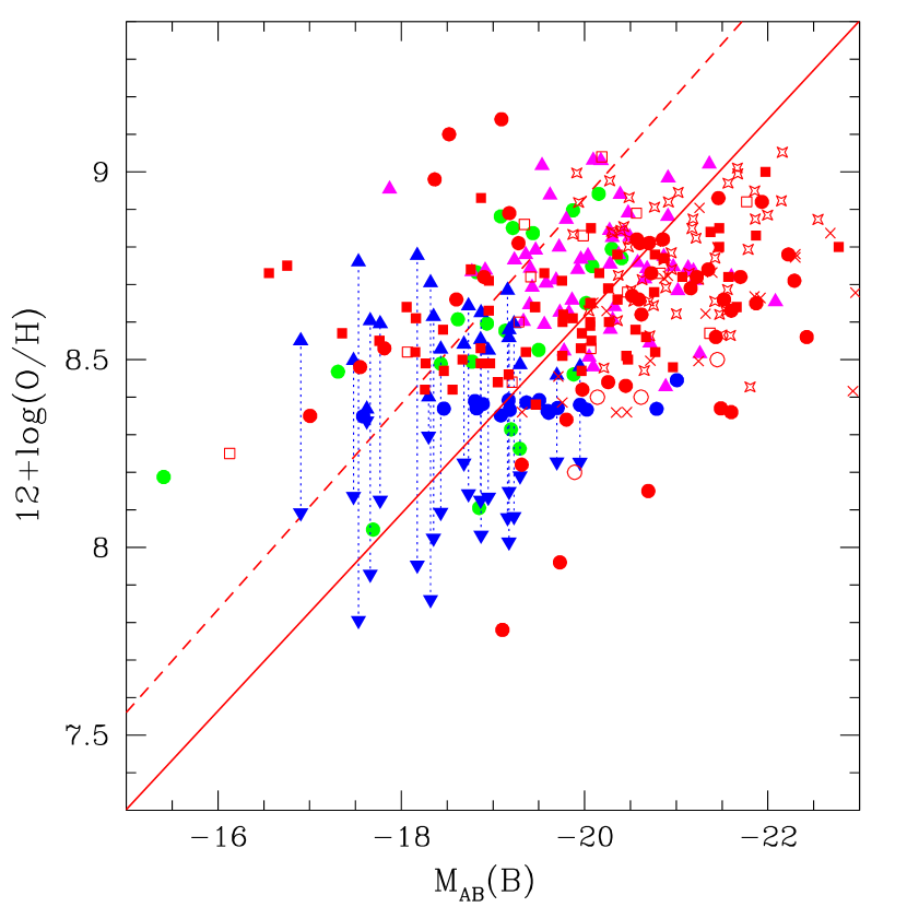
Figure 10: The $L-Z$ relation including additional samples of intermediate-redshift galaxies and using metallicities derived with the $R_{\mathrm{23}}$ method. Green filled circles are objects where N2 diagnostic is used for metallicity estimate, magenta triangles are objects with a secure $L$ diagnostic, and blue triangles are objects with an unreliable diagnostic (for these objects the two possible abundances are shown). Other samples of intermediate-redshift galaxies drawn from the literature are plotted in red: open squares from Kobulnicky & Zaritsky (1999), solid squares from Kobulnicky et al. (2003), open circles from Hammer et al. (2001), filled circles from Liang et al. (2004), stars from Lilly et al. (2003) and crosses from Contini et al. (2002) ($z>0.1$). The solid line shows the linear regression for all these points, compared to the relation obtained in the local universe from 2dFGRS data (dashed line).

Figure 11: Selection effects when we include other samples of intermediate-redshift galaxies drawn from the literature (see text for details). This figure shows, as a function of redshift, the distribution of the absolute $B$-band magnitudes (bottom panel) and metallicities (top panel) of the combined sample of intermediate-redshift galaxies. The straight line shows the linear regression of the observed (not real) evolution. Histograms are plotted for four redshift bins: $0.2\leq z\leq 0.4$, $0.4<z\leq 0.6$, $0.6<z\leq 0.8$ and $z>0.8$.

3.3 Different regimes of the $L-Z$ relation

Different authors (e.g. Melbourne & Salzer 2002; Lamareille et al. 2004) have suggested that the global $L-Z$ relation in the local universe may not be simply approximated by a single linear relation and proposed to divide the galaxy samples into metal-poor dwarfs and metal-rich spirals. The $L-Z$ relations derived for these two subsamples by Lamareille et al. (2004) are indeed different, with metal-rich galaxies following a steeper $L-Z$ relation than the metal-poor ones.

We can try to apply this distinction between metal-poor and metal-rich galaxies to our samples of intermediate-redshift galaxies, in order to derive “metallicity-dependant” $L-Z$ relations. However, we believe that a constant limit in metallicity to separate the two galaxy populations (e.g. $12+\log(\textrm{O}/\textrm{H})=8.3$ as used in Lamareille et al. 2004) is not the best way to do as it does not take into account accurately the high dispersion of observed metallicities at a given galaxy luminosity. Indeed there is no clear physical separation between galaxies having a metallicity lower or higher than one specific value.

Instead, taking into account the intrinsic scatter of the $L-Z$ relation, we try in this section to define a “region fitting” which gives the behavior of the $L-Z$ relation in a metal-rich and a metal-poor regimes (i.e. respectively the upper and the lower regions of the $L-Z$ relation). We assume that the separation between metal-rich and metal-poor galaxies increases with the absolute magnitude with a similar slope of $-0.27$ than for the $L-Z$ relation in the local universe from the 2dFGRS. The separation between metal-poor and metal-rich galaxies is thus equal to the mean metallicity of a galaxy at a given luminosity. Note that this method is not sensitive to whether the physical mixing of galaxies in the $L-Z$ diagram is done along the x-axis or along the y-axis (if the mixing is done along the x-axis, this is rather a high/low-luminosity separation).

We emphasize that we do not use the standard, horizontal, separation between low- and high-metallicity objects described in Sect. 2.1.1. We use instead a luminosity-dependant separation which gives us $61$ metal-poor and $59$ metal-rich galaxies. Please note that in order to take into account the lower average metallicity of our sample (see Fig. 7), we have shifted our luminosity-dependent separation between metal-rich and metal-poor galaxies towards lower metallicities by $-0.20$ dex, keeping the same slope given by the local $L-Z$ relation.

We have applied this method to divide our sample of intermediate-redshift galaxies into metal-rich and metal-poor galaxies using the $L-Z$ relation derived in the local universe from the 2dFGRS data. The two new linear fits obtained for each sub-sample are shown in Fig. 12. We derive the following relations:

$$12+\log(\textrm{O/H})=-(0.26\pm 0.02)M_{AB}(B)+3.30\pm 0.38$$ (5)

for metal-poor galaxies, and

$$12+\log(\textrm{O/H})=-(0.24\pm 0.03)M_{AB}(B)+4.15\pm 0.49$$ (6)

for metal-rich galaxies. The rms of the residuals for the whole sample is now equal to $0.15$ dex only, and we see on the bottom panel of Fig. 12 that there is almost no residual slope. This has to be compared with the quite high dispersion (rms $\sim 0.28-0.34$ dex) and the non-zero slope of the residuals obtained for the single $L-Z$ relation (see Fig. 7).

Figure 12: The “region-fitted” $L-Z$ relations for our own sample of intermediate-redshift galaxies. The metallicities are derived with the $R_{\mathrm{23}}$ method. The solid lines represent the two linear regressions for the metal-poor and metal-rich galaxies (see text for details). Same legend as in Fig. 7 for the data points. The bottom panel shows the residuals around these two fits.

The same distinction between metal-poor and metal-rich galaxies can be applied to the whole sample of intermediate-redshift galaxies, i.e. adding the samples drawn from the literature (see Sect. 3.2).

The two new linear fits obtained for each sub-sample (the separation is shifted by $-0.32$ dex) are shown in Fig. 13. We derive the following relations:

$$12+\log(\textrm{O/H})=-(0.27\pm 0.03)M_{AB}(B)+2.96\pm 0.53$$ (7)

for $184$ metal-poor galaxies , and

$$12+\log(\textrm{O/H})=-(0.21\pm 0.01)M_{AB}(B)+4.65\pm 0.29$$ (8)

for $164$ metal-rich galaxies. The rms of the residuals for the whole sample is equal to $0.19$ dex and we see again on the bottom panel of Fig. 13 that there is almost no residual slope.

The metallicity-dependent $L-Z$ relations derived above are very similar, in terms of slope and zero point, if we consider our sample alone or the whole sample of intermediate-redshift galaxies.

Figure 13: The “region-fitted” $L-Z$ relations including additional samples of intermediate-redshift galaxies (as described in Sect. 3.2). The metallicities are derived with the $R_{\mathrm{23}}$ method. The solid lines represent the two linear regressions for the metal-poor and metal-rich galaxies (see text for details). Same legend as in Fig. 7 for the data points. The bottom panel shows the residuals around these two fits.

3.4 Evolution of the $L-Z$ relation with redshift?

We now investigate a possible evolution with redshift of the $L-Z$ relation, using the $R_{\mathrm{23}}$ method for the metallicity determination.

We first divided our own sample of intermediate-redshift galaxies into four redshift bins: $0.2\leq z\leq 0.4$, $0.4<z\leq 0.6$, $0.6<z\leq 0.8$ and $0.8<z<1.0$.

The resulting $L-Z$ relations per redshift bin are shown in Fig. 14. The parameters (slope, zero points) of the linear regressions are listed in Table 2. The parameter $f_{\mathrm{above}}$ corresponds to the fraction of galaxies located above the local $L-Z$ relation derived with 2dFGRS data.

With the present sample, we only see a small, not significant, evolution of the $L-Z$ relation with redshift, in terms of slope and zero point, from the local universe to $z\sim 1$. We only find statistical variations consistent with the uncertainty in the derived parameters. The small variation is however confirmed by a decreasing fraction of galaxies falling above the local $L-Z$ relation ($f_{\mathrm{above}}$ in Table 2).

Figure 14: Redshift evolution of the $L-Z$ relation (see text for details). The four panels show the $L-Z$ relation for our own sample of intermediate-redshift galaxies in the redshift ranges $0.2\leq z\leq 0.4$, $0.4<z\leq 0.6$, $0.6<z\leq 0.8$ and $0.8<z<1.0$. The legend is the same as in Fig. 7.

Table 2: Redshift evolution of the slope, zero point and rms of the residuals of the $L-Z$ relation for our own sample of intermediate-redshift star-forming galaxies. Metallicities have been estimated with the $R_{\mathrm{23}}$ method. The parameter $f_{\mathrm{above}}$ represents the fraction of galaxies located above the local $L-Z$ relation. The results obtained on the 2dFGRS sample (Lamareille et al. 2004) are given for reference.

Redshift bin	Slope	Zero Point	rms	$f_{\mathrm{above}}$
2dFGRS	$-0.27\pm 0.01$	$3.45\pm 0.09$	$0.27$
$0.2\leq z\leq 0.4$	$-0.34\pm 0.05$	$2.06\pm 0.98$	$0.27$	$0.45$
$0.4<z\leq 0.6$	$-0.27\pm 0.06$	$3.18\pm 1.24$	$0.30$	$0.30$
$0.6<z\leq 0.8$	$-0.28\pm 0.04$	$3.01\pm 0.85$	$0.17$	$0.15$
$0.8<z<1.0$	$-0.29\pm 0.17$	$2.74\pm 3.44$	$0.27$	$0.10$

In order to be more complete in searching for any possible evolution of the $L-Z$ relation with redshift, Fig. 15 and Table 3 show the $L-Z$ relation with the addition of other samples of intermediate-redshift galaxies (as described in Sect. 3.2) divided into four redshift bins: $0.2\leq z\leq 0.4$, $0.4<z\leq 0.6$, $0.6<z\leq 0.8$ and $0.8<z<1.0$.

As previously observed with our sample alone, the $L-Z$ relation only shows a small evolution, in terms of slope and zero points, between these four redshift bins. Again, we only find statistical variations consistent with the uncertainty in the derived parameters (see Table 3).

However, we remark that the $L-Z$ relation tends to shift toward lower metallicities when the redshift increases, which is confirmed by a decrease of the fraction of galaxies $f_{\mathrm{above}}$ above the local $L-Z$ relation (from $43$% at $z\sim 0.3$ to $3$% at $z\sim 1$, see Table 3).

Figure 15: Redshift evolution of the $L-Z$ relation using the $R_{\mathrm{23}}$ method for the metallicity determination and including other samples of intermediate-redshift galaxies (as described in Sect. 3.2). The four panels show the $L-Z$ relation for the full combined sample in the redshift ranges $0.2\leq z\leq 0.4$, $0.4<z\leq 0.6$, $0.6<z\leq 0.8$ and $0.8<z<1.0$. The legend is the same as in Fig. 10.

Table 3: Redshift evolution of the slope, zero point and rms of the residuals of the $L-Z$ relation including other samples of intermediate-redshift galaxies (as described in Sect. 3.2). Metallicities have been estimated with the $R_{\mathrm{23}}$ method. The parameter $f_{\mathrm{above}}$ represents the fraction of galaxies located above the local $L-Z$ relation.

Redshift bin	Slope	Zero Point	rms	$f_{\mathrm{above}}$
$0.2\leq z\leq 0.4$	$-0.34\pm 0.10$	$1.98\pm 1.85$	$0.43$	$0.43$
$0.4<z\leq 0.6$	$-0.37\pm 0.09$	$1.10\pm 1.86$	$0.39$	$0.22$
$0.6<z\leq 0.8$	$-0.28\pm 0.04$	$3.04\pm 0.81$	$0.23$	$0.07$
$0.8<z<1.0$	$-0.28\pm 0.08$	$2.86\pm 1.72$	$0.27$	$0.03$

To better quantify this possible evolutionary effect, we estimate for each galaxy with a given luminosity, the difference between its metallicity and the one given by the $L-Z$ relation in the local universe. For each redshift bin, the mean value of this difference give us the average metallicity shift, assuming that, in average, the metallicity increases with the galaxy luminosity with a slope equal to $-0.27$ (see Table 2). The results are shown in Table 4 (case a). We clearly see a decrease of the mean metallicity for a given luminosity when the redshift increases. The last column shows that the galaxies in the redshift range $0.8<z<1.0$ appear to be metal-deficient by a factor of $\sim 3$ compared with galaxies in the local universe. For a given luminosity, they contain on average about third of the metals locked in local galaxies.

We acknowledge that the evolution of the $L-Z$ relation is a combination of a metallicity and a luminosity evolution at a given stellar mass. Unfortunately our sample is not large enough to statistically distinguish between the two effects, but for the convenience of the reader we have done the same calculations after correcting the luminosity of the galaxies from the evolution. The results are listed in Table 4 (case b). We have used the last results obtained on the evolution of the galaxy luminosity function in the VVDS first epoch data (Ilbert et al. 2004), which give an average evolution in the $B$-band magnitude of $-0.3$ at $z=0.2$, $-0.7$ at $z=0.4$, $-0.9$ at $z=0.8$ and $-1.0$ at $z=1.0$ since $z=0.0$. If these values correctly reflect the luminosity evolution of our sample, the metallicity decrease at redshift up to $z=1.0$ would be of a factor $\sim 1.3$ for a given stellar mass (if we neglect the effect of the different mass-to-light ratios).

Table 4: Evolution with redshift of the mean value of the metallicity difference with the $L-Z$ relation in the local universe. The average difference of metallicity (derived with the $R_{\mathrm{23}}$ method) is computed for four redshift bins for our sample of star-forming galaxies, including other samples of intermediate-redshift galaxies (as described in Sect. 3.2). Case (a) is uncorrected data, case (b) is after the luminosities have been corrected from evolution (see text for details). The two last columns show the same value converted into a linear scale. It indicates the amount of metals in each redshift bin compared with the value in the local universe.

	$\left\langle Z-Z_{2dF}(L)\right\rangle$		linear
Redshift bin	(a)	(b)	(a)	(b)
$0.2\leq z\leq 0.4$	$-0.16$	$-0.08$	$0.97$	$1.17$
$0.4<z\leq 0.6$	$-0.33$	$-0.14$	$0.60$	$0.93$
$0.6<z\leq 0.8$	$-0.38$	$-0.14$	$0.47$	$0.83$
$0.8<z<1.0$	$-0.55$	$-0.28$	$0.34$	$0.64$

4 Conclusion

Starting with a sample of 129 star-forming galaxies at intermediate redshifts ($0.2<z<1.0$), for which the sample selection, the observations and associated data reduction, the photometric properties, the emission-line measurements, and the spectral classification are described in Paper I, we derived the gas-phase oxygen abundance O/H which is used as a tracer of the metallicity. We used two methods: the $R_{\mathrm{23}}$ method (McGaugh 1991) which is based on empirical calibrations, and the CL01 method (Charlot & Longhetti 2001) which is based on grids of photo-ionization models and on fitting emission lines. We have investigated the problem of the metallicity degeneracy between the high- and low-metallicity branches of the O/H vs. $R_{\mathrm{23}}$ relationship. The following conclusions have been drawn from this study:

• The N2 diagnostic based on the [Nii]$\lambda 6584$/H$\alpha$ line ratio is the best way to discriminate between high- and low-metallicity objects.

• The $L$ diagnostic can be used with a relatively high confidence level for galaxies far enough from the turnaround region (12+log(O/H) $\sim 8.3$) of the O/H vs. $R_{\mathrm{23}}$ relationship. Note however that, in this region, the error in the final abundance will be low.

• Any diagnostic based on the galaxy color or the intensity of the Balmer break will fail because of the high dispersion in the relations between metallicity and these parameters.

• The CL01 method offers a good way to break the metallicity degeneracy with the maximum likelihood method, even when the [Nii]$\lambda 6584$ and H$\alpha$ lines are not available.

We have then derived the following luminosity – metallicity ($L-Z$) relations: the $L-Z$ relation in the $B$-band and in the $R$-band using the $R_{\mathrm{23}}$ method for metallicity determinations (equations 1 and 2), the $L-Z$ relation in the $B$-band with the CL01 method to derive metallicities (equation 3), and the $L-Z$ relation for our galaxies combined with other samples of intermediate-redshift galaxies drawn from the literature (see Sect. 3.2) and the $R_{\mathrm{23}}$ method for metallicity estimates (equation 4). We investigated the possibility to divide, for a given luminosity, the sample into metal-rich and metal-poor galaxies in order to do a “region fitting” instead of a single linear fit. We thus derived two new $L-Z$ relations showing similar slopes but lower residuals (equations 7 and 8). We draw the following conclusions from this analysis:

• The $L-Z$ relations at intermediate redshifts are very similar in term of slope to the $L-Z$ relations obtained in the local universe (Lamareille et al. 2004; Tremonti et al. 2004).

• When including other samples of intermediate-redshift galaxies (see Sect. 3.2), we find a $L-Z$ relation which is shifted by $\sim 0.3$ dex towards lower metallicities compared with the local one.

Finally, we investigated any possible evolution of these $L-Z$ relations with redshift. We find that:

• Our sample alone does not show any significant evolution of the $L-Z$ relation up to $z\sim 1.0$. We only find statistical variations consistent with the uncertainty in the derived parameters.

• Including other samples of intermediate-redshift galaxies (see Sect. 3.2), we clearly see, at a given galaxy luminosity, a decrease of the mean metallicity when the redshift increases. Galaxies at $z\sim 1$ appear to be metal-deficient by a factor of $\sim 3$ compared with galaxies in the local universe. For a given luminosity, they contain on average about one third of the metals locked in local galaxies.

• If we apply a correction for the luminosity evolution, galaxies at $z\sim 1$ appear to be metal-deficient by a factor of $\sim 1.6$ compared with galaxies in the local universe.

Further analysis of our sample of intermediate-redshift galaxies, in terms of mass and star formation history, will be performed in subsequent papers.

[x]llrrrrllr Gas-phase oxygen abundances (computed with the $R_{\mathrm{23}}$ method) of star-forming galaxies at intermediate redshifts. LCL05: identification number, ^∗ flag for candidate star-forming galaxies (see Paper I). alt: alternative identification if available. z: redshift. M(B): absolute magnitude in the $B$ band (AB system). low: lower branch metallicity. high: higher branch metallicity. N2: metallicity regime with the N2 diagnostic (“med” stands for galaxies with O/H_low greater than O/H_high which are kept as intermediate metallicity objects, see text for details). LZ: metallicity regime with the $L$ diagnostic (object with an unreliable $L$ diagnostic are flagged by a ‘*’). 12+log(O/H): adopted abundance.
LCL05 alt z $M(B)$ low high N2 LZ 12+log(O/H)
continued
LCL05 alt z $M(B)$ low high N2 LZ 12+log(O/H)
001 $0.341$ $-19.47$ $7.90$ $8.79$ … high $8.79\pm 0.07$
002 $0.616$ $-21.36$ $7.38$ $9.02$ … high $9.02\pm 0.03$
003 $0.341$ $-20.31$ $8.04$ $8.61$ … high $8.61\pm 0.03$
004 CFRS$ $00.0852 $0.268$ $-20.30$ $8.02$ $8.79$ high high $8.79\pm 0.05$
006 CFRS$ $00.0900 $0.247$ $-18.85$ $8.10$ $8.56$ low high${}^{\textrm{*}}$ $8.10\pm 0.11$
007 CFRS$ $00.0940 $0.269$ $-19.88$ $8.39$ $8.46$ high high${}^{\textrm{*}}$ $8.46\pm 0.28$
008 CFRS$ $00.1013 $0.244$ $-19.13$ $8.13$ $8.58$ high high${}^{\textrm{*}}$ $8.58\pm 0.06$
009 CFRS$ $00.0124 $0.288$ $-20.08$ $7.96$ $8.75$ high high $8.75\pm 0.06$
010 CFRS$ $00.0148 $0.267$ $-18.93$ $8.19$ $8.60$ high high${}^{\textrm{*}}$ $8.60\pm 0.14$
011 CFRS$ $00.1726 $0.296$ $-19.95$ $8.58$ $8.18$ med med $8.38\pm 0.30$
013 $0.249$ $-18.73$ $8.14$ $8.64$ … high${}^{\textrm{*}}$ $8.64\pm 0.18$
014 $0.390$ $-20.27$ $7.82$ $8.84$ … high $8.84\pm 0.08$
015 CFRS$ $00.1057 $0.243$ $-17.31$ $8.19$ $8.47$ high low${}^{\textrm{*}}$ $8.47\pm 0.10$
016 CFRS$ $00.0121 $0.297$ $-19.29$ $8.26$ $8.41$ low high${}^{\textrm{*}}$ $8.26\pm 0.03$
018^∗ CFRS$ $03.1184 $0.205$ $-18.46$ $8.55$ $8.19$ med med $8.37\pm 0.29$
020 CFRS$ $03.0442 $0.478$ $-19.86$ $8.04$ $8.66$ … high $8.66\pm 0.25$
021 CFRS$ $03.0476 $0.260$ $-18.87$ $8.13$ $8.55$ … high${}^{\textrm{*}}$ $8.55\pm 0.04$
022 CFRS$ $03.0488 $0.605$ $-20.66$ $7.88$ $8.71$ … high $8.71\pm 0.06$
023 CFRS$ $03.0507 $0.465$ $-20.86$ $7.84$ $8.77$ … high $8.77\pm 0.03$
024 CFRS$ $03.0523 $0.653$ $-21.02$ $7.93$ $8.68$ … high $8.68\pm 0.05$
025^∗ CFRS$ $03.0578 $0.219$ $-19.18$ $8.52$ $8.21$ med med $8.37\pm 0.31$
026 CFRS$ $03.0605 $0.219$ $-16.90$ $8.09$ $8.55$ … low${}^{\textrm{*}}$ $8.09\pm 0.08$
027^∗ CFRS$ $03.0003 $0.219$ $-17.48$ $8.14$ $8.50$ … low${}^{\textrm{*}}$ $8.14\pm 0.13$
028 CFRS$ $03.0037 $0.174$ $-19.50$ $8.23$ $8.53$ high high${}^{\textrm{*}}$ $8.53\pm 0.03$
029 CFRS$ $03.0046 $0.512$ $-20.88$ $8.33$ $8.43$ … high $8.43\pm 0.32$
030 CFRS$ $03.0085 $0.608$ $-20.30$ $7.71$ $8.82$ … high $8.82\pm 0.16$
031 CFRS$ $03.0096 $0.219$ $-17.58$ $8.36$ $8.34$ med med $8.35\pm 0.23$
032 CFRS$ $22.0502 $0.468$ $-19.72$ $7.89$ $8.80$ … high $8.80\pm 0.06$
034 CFRS$ $22.0671 $0.318$ $-19.20$ $8.31$ $8.42$ low high${}^{\textrm{*}}$ $8.31\pm 0.07$
035 CFRS$ $22.0819 $0.291$ $-19.36$ $7.89$ $8.78$ … high $8.78\pm 0.05$
036 CFRS$ $22.0855 $0.210$ $-18.77$ $8.19$ $8.49$ high high${}^{\textrm{*}}$ $8.49\pm 0.03$
038 CFRS$ $22.1013 $0.231$ … $8.12$ $8.57$ high … $8.57\pm 0.03$
039 CFRS$ $22.1084 $0.293$ $-20.02$ $8.09$ $8.65$ high high $8.65\pm 0.06$
040 CFRS$ $22.1203 $0.538$ $-20.58$ $7.81$ $8.76$ … high $8.76\pm 0.03$
041 $0.216$ $-18.80$ $8.63$ $8.15$ med med $8.39\pm 0.31$
042 $0.352$ $-18.77$ $7.80$ $8.73$ … high $8.73\pm 0.04$
043 CFRS$ $22.0622 $0.324$ $-18.17$ $7.95$ $8.78$ … high${}^{\textrm{*}}$ $8.78\pm 0.10$
044 $0.276$ $-19.80$ $7.74$ $8.87$ … high $8.87\pm 0.05$
046 $0.651$ $-20.47$ $7.64$ $8.89$ … high $8.89\pm 0.04$
047 $0.472$ $-18.35$ $8.02$ $8.62$ … high${}^{\textrm{*}}$ $8.62\pm 0.11$
049 CFRS$ $22.0832 $0.231$ $-19.09$ $7.79$ $8.88$ high high $8.88\pm 0.04$
050 CFRS$ $22.1064 $0.537$ $-19.96$ $7.78$ $8.77$ … high $8.77\pm 0.04$
051^∗ CFRS$ $22.1339 $0.384$ $-19.33$ $7.97$ $8.60$ … high $8.60\pm 0.02$
052 CFRS$ $22.0474 $0.279$ $-18.62$ $7.97$ $8.61$ high high${}^{\textrm{*}}$ $8.61\pm 0.02$
053 CFRS$ $22.0504 $0.538$ $-21.13$ $7.86$ $8.74$ … high $8.74\pm 0.03$
054 CFRS$ $22.0637 $0.542$ $-21.19$ $7.85$ $8.74$ … high $8.74\pm 0.03$
055 CFRS$ $22.0642 $0.469$ $-21.20$ $7.92$ $8.71$ … high $8.71\pm 0.05$
056 CFRS$ $22.0717 $0.279$ $-20.15$ $7.72$ $8.94$ high high $8.94\pm 0.04$
057 CFRS$ $22.0823 $0.333$ $-20.71$ $8.18$ $8.54$ … high $8.54\pm 0.09$
058 CFRS$ $22.1082 $0.292$ $-19.83$ $7.93$ $8.62$ … high $8.62\pm 0.05$
059 $0.277$ $-19.58$ $7.99$ $8.70$ … high $8.70\pm 0.05$
060 CFRS$ $22.1144 $0.359$ $-19.23$ $8.08$ $8.60$ … high${}^{\textrm{*}}$ $8.60\pm 0.08$
061 CFRS$ $22.1220 $0.358$ $-19.81$ $8.14$ $8.62$ … high $8.62\pm 0.04$
062 CFRS$ $22.1231 $0.285$ $-19.22$ $7.82$ $8.85$ high high $8.85\pm 0.02$
063 CFRS$ $22.1309 $0.285$ $-18.87$ $8.03$ $8.62$ … high${}^{\textrm{*}}$ $8.62\pm 0.05$
065 $0.066$ $-15.41$ $8.19$ $8.46$ low low $8.19\pm 0.01$
067 $0.450$ $-19.18$ $8.15$ $8.58$ … high${}^{\textrm{*}}$ $8.58\pm 0.12$
068 $0.629$ $-19.70$ $8.54$ $8.20$ med med $8.37\pm 0.63$
069 $0.221$ $-18.43$ $8.23$ $8.49$ high high${}^{\textrm{*}}$ $8.49\pm 0.07$
070 $0.739$ $-20.39$ $7.57$ $8.94$ … high $8.94\pm 0.02$
071 $0.526$ $-20.28$ $8.15$ $8.58$ … high $8.58\pm 0.04$
072 $0.342$ $-18.92$ $7.93$ $8.74$ … high $8.74\pm 0.06$
073 LBP2003 b $0.260$ $-19.44$ $7.85$ $8.84$ high high $8.84\pm 0.02$
076 LBP2003 h $0.321$ $-20.40$ $7.96$ $8.77$ high high $8.77\pm 0.03$
077 LBP2003 c $0.300$ $-19.87$ $7.74$ $8.90$ high high $8.90\pm 0.03$
078 CPK2001 V7 $0.567$ $-20.97$ $7.92$ $8.75$ … high $8.75\pm 0.06$
079 CPK2001 V6 $0.410$ $-19.16$ $8.08$ $8.68$ … high${}^{\textrm{*}}$ $8.68\pm 0.11$
080 CBB2001 688 $0.330$ $-18.82$ $7.90$ $8.73$ high high $8.73\pm 0.03$
081 CPK2001 V11 $0.380$ $-17.53$ $7.80$ $8.76$ … low${}^{\textrm{*}}$ $7.80\pm 0.15$
083 $0.726$ $-20.05$ $8.14$ $8.51$ … high $8.51\pm 0.04$
084 CBB2001 453 $0.410$ $-18.82$ $8.62$ $8.12$ med med $8.37\pm 0.26$
085^∗ $0.719$ $-19.59$ $8.47$ $8.26$ med med $8.36\pm 0.52$
086 $0.412$ $-19.95$ $8.23$ $8.48$ … high${}^{\textrm{*}}$ $8.48\pm 0.11$
087 $0.409$ $-18.32$ $7.86$ $8.70$ … high${}^{\textrm{*}}$ $8.70\pm 0.06$
088^∗ $0.757$ $-19.78$ $8.08$ $8.52$ … high $8.52\pm 0.05$
089^∗ $0.563$ $-20.02$ $8.71$ $8.02$ med med $8.37\pm 0.36$
091 $0.786$ $-19.41$ $7.83$ $8.74$ … high $8.74\pm 0.06$
092^∗ $0.329$ $-18.43$ $8.09$ $8.53$ … high${}^{\textrm{*}}$ $8.53\pm 0.02$
093 $0.640$ $-20.33$ $7.98$ $8.64$ … high $8.64\pm 0.06$
095 $0.342$ $-17.87$ $7.47$ $8.95$ … high $8.95\pm 0.02$
096 $0.439$ $-19.37$ $8.40$ $8.37$ med med $8.39\pm 0.28$
098 $0.572$ $-17.62$ $8.34$ $8.37$ … low${}^{\textrm{*}}$ $8.34\pm 0.32$
099 $0.355$ $-19.93$ $7.95$ $8.74$ … high $8.74\pm 0.05$
100 $0.355$ $-19.40$ $8.01$ $8.65$ … high $8.65\pm 0.05$
101 $0.355$ $-19.50$ $8.56$ $8.23$ med med $8.39\pm 0.35$
102 $0.428$ $-21.01$ $8.59$ $8.30$ med med $8.45\pm 0.28$
103 $0.476$ $-21.26$ $8.23$ $8.52$ … high $8.52\pm 0.07$
104 $0.452$ $-20.04$ $7.98$ $8.78$ … high $8.78\pm 0.07$
105^∗ GDDS$ $02-0452 $0.828$ $-20.79$ $8.75$ $7.99$ med med $8.37\pm 0.43$
106 GDDS$ $02-0585 $0.825$ $-19.70$ $8.23$ $8.46$ … high${}^{\textrm{*}}$ $8.46\pm 0.17$
107 GDDS$ $02-0756 $0.864$ $-18.89$ $8.57$ $8.20$ med med $8.38\pm 0.37$
108 GDDS$ $02-0995 $0.786$ $-19.17$ $8.55$ $8.23$ med med $8.39\pm 0.53$
110 GDDS$ $02-1724 $0.996$ $-22.08$ $7.88$ $8.65$ … high $8.65\pm 0.16$
112 GDDS$ $12-5513 $0.611$ $-20.43$ $7.86$ $8.84$ … high $8.84\pm 0.03$
113 GDDS$ $12-5685 $0.960$ $-20.68$ $7.84$ $8.74$ … high $8.74\pm 0.10$
114 GDDS$ $12-5722 $0.841$ $-20.28$ $7.90$ $8.75$ … high $8.75\pm 0.07$
116 GDDS$ $12-6800 $0.615$ $-21.60$ $7.92$ $8.72$ … high $8.72\pm 0.13$
117 GDDS$ $12-7099 $0.567$ $-20.09$ $7.60$ $9.03$ … high $9.03\pm 0.01$
118 GDDS$ $12-7205 $0.568$ $-19.54$ $7.41$ $9.02$ … high $9.02\pm 0.01$
119 GDDS$ $12-7660 $0.791$ $-20.49$ $7.81$ $8.83$ … high $8.83\pm 0.03$
120 GDDS$ $12-7939 $0.664$ $-18.95$ $8.13$ $8.53$ … high${}^{\textrm{*}}$ $8.53\pm 0.09$
122 GDDS$ $22-0040 $0.818$ $-19.73$ $7.97$ $8.63$ … high $8.63\pm 0.07$
123 GDDS$ $22-0145 $0.754$ $-19.43$ $7.91$ $8.69$ … high $8.69\pm 0.04$
124 GDDS$ $22-0563 $0.787$ $-20.37$ $7.82$ $8.78$ … high $8.78\pm 0.02$
125 GDDS$ $22-0619 $0.673$ $-18.68$ $8.22$ $8.54$ … high${}^{\textrm{*}}$ $8.54\pm 0.22$
126 GDDS$ $22-0630 $0.753$ $-20.18$ $7.24$ $9.03$ … high $9.03\pm 0.01$
127 GDDS$ $22-0643 $0.788$ $-19.56$ $8.11$ $8.59$ … high $8.59\pm 0.14$
129 GDDS$ $22-0926 $0.786$ $-19.30$ $8.19$ $8.49$ … high${}^{\textrm{*}}$ $8.49\pm 0.14$
131 GDDS$ $22-1674 $0.879$ $-19.23$ $7.70$ $8.77$ … high $8.77\pm 0.03$
132 GDDS$ $22-2196 $0.627$ $-18.30$ $8.30$ $8.40$ … high${}^{\textrm{*}}$ $8.40\pm 0.18$
133 GDDS$ $22-2491 $0.471$ $-17.69$ $8.05$ $8.56$ low low${}^{\textrm{*}}$ $8.05\pm 0.08$
134 GDDS$ $22-2541 $0.617$ $-19.69$ $7.96$ $8.71$ … high $8.71\pm 0.06$
135 GDDS$ $22-2639 $0.883$ $-20.91$ $7.54$ $8.88$ … high $8.88\pm 0.01$
136 SKK2001 368 $0.693$ $-20.91$ $7.64$ $8.98$ … high $8.98\pm 0.04$
137 SKK2001 159 $0.473$ $-19.62$ $7.75$ $8.94$ … high $8.94\pm 0.04$
138 $0.449$ $-17.77$ $8.13$ $8.60$ … low${}^{\textrm{*}}$ $8.13\pm 0.19$
140^∗ $0.731$ $-19.61$ $8.40$ $8.32$ med med $8.36\pm 0.36$
141 $0.398$ $-19.09$ $8.88$ $7.83$ med med $8.35\pm 0.81$

[x]llrrrrrr Gas-phase oxygen abundances (with the CL01 method) of star-forming galaxies at intermediate redshifts. LCL05: identification number, ^∗ flag for candidate star-forming galaxies (see Paper I). alt: alternative identification if available. low: lower peak metallicity. $A_{l}$: associated likelihood amplitude. $P_{l}$: associated probability. high: higher peak metallicity. $A_{h}$: associated likelihood amplitude. $P_{h}$: associated probability. The boldface values designate the highest likelihood and the adopted abundances.
LCL05 alt low $A_{l}$ $P_{l}$ high $A_{h}$ $P_{h}$
continued
LCL05 alt low $A_{l}$ $P_{l}$ high $A_{h}$ $P_{h}$
001 $7.80\pm 0.08$ $0.33$ $0.03$ $\mathbf{8.88\pm 0.10}$ $\mathbf{9.64}$ $\mathbf{0.97}$
002 $7.75\pm 0.07$ $0.01$ $0.00$ $\mathbf{9.10\pm 0.09}$ $\mathbf{10.56}$ $\mathbf{1.00}$
003 $8.21\pm 0.21$ $2.78$ $0.45$ $\mathbf{8.65\pm 0.11}$ $\mathbf{3.35}$ $\mathbf{0.55}$
004 CFRS$ $00.0852 $8.30\pm 0.35$ $0.02$ $0.00$ $\mathbf{8.79\pm 0.02}$ $\mathbf{33.43}$ $\mathbf{1.00}$
006 CFRS$ $00.0900 $\mathbf{8.06\pm 0.08}$ $\mathbf{6.65}$ $\mathbf{0.72}$ $8.28\pm 0.17$ $2.63$ $0.28$
007 CFRS$ $00.0940 $7.97\pm 0.12$ $1.33$ $0.12$ $\mathbf{8.82\pm 0.08}$ $\mathbf{9.76}$ $\mathbf{0.88}$
008 CFRS$ $00.1013 $8.30\pm 0.15$ $2.23$ $0.20$ $\mathbf{8.67\pm 0.07}$ $\mathbf{8.98}$ $\mathbf{0.80}$
009 CFRS$ $00.0124 $8.81\pm 0.07$ $5.16$ $0.26$ $\mathbf{8.88\pm 0.04}$ $\mathbf{14.95}$ $\mathbf{0.74}$
010 CFRS$ $00.0148 $8.75\pm 0.01$ $1.65$ $0.11$ $\mathbf{8.94\pm 0.07}$ $\mathbf{13.73}$ $\mathbf{0.89}$
011 CFRS$ $00.1726 $\mathbf{8.41\pm 0.09}$ $\mathbf{7.34}$ $\mathbf{0.53}$ $8.44\pm 0.06$ $6.40$ $0.47$
012 CFRS$ $00.0699 $\mathbf{8.38\pm 0.29}$ $\mathbf{3.11}$ $\mathbf{0.70}$ $8.44\pm 0.07$ $1.33$ $0.30$
013 $8.26\pm 0.31$ $0.89$ $0.14$ $\mathbf{8.75\pm 0.13}$ $\mathbf{5.70}$ $\mathbf{0.86}$
014 $7.80\pm 0.09$ $0.23$ $0.02$ $\mathbf{9.04\pm 0.10}$ $\mathbf{9.13}$ $\mathbf{0.98}$
015 CFRS$ $00.1057 $8.18\pm 0.15$ $3.24$ $0.47$ $\mathbf{8.58\pm 0.13}$ $\mathbf{3.70}$ $\mathbf{0.53}$
016 CFRS$ $00.0121 $8.22\pm 0.02$ $13.40$ $0.31$ $\mathbf{8.41\pm 0.02}$ $\mathbf{29.70}$ $\mathbf{0.69}$
018^∗ CFRS$ $03.1184 $8.19\pm 0.06$ $1.32$ $0.15$ $\mathbf{8.44\pm 0.12}$ $\mathbf{7.34}$ $\mathbf{0.85}$
019 CFRS$ $03.1343 $\mathbf{8.11\pm 0.12}$ $\mathbf{6.37}$ $\mathbf{0.82}$ $8.36\pm 0.14$ $1.44$ $0.18$
020 CFRS$ $03.0442 $8.19\pm 0.24$ $2.29$ $0.46$ $\mathbf{8.69\pm 0.17}$ $\mathbf{2.65}$ $\mathbf{0.54}$
021 CFRS$ $03.0476 $8.05\pm 0.08$ $6.16$ $0.21$ $\mathbf{8.06\pm 0.02}$ $\mathbf{23.80}$ $\mathbf{0.79}$
022 CFRS$ $03.0488 $8.20\pm 0.21$ $2.79$ $0.47$ $\mathbf{8.65\pm 0.13}$ $\mathbf{3.16}$ $\mathbf{0.53}$
023 CFRS$ $03.0507 $8.21\pm 0.30$ $2.29$ $0.47$ $\mathbf{8.80\pm 0.12}$ $\mathbf{2.54}$ $\mathbf{0.53}$
024 CFRS$ $03.0523 $8.16\pm 0.24$ $2.30$ $0.44$ $\mathbf{8.70\pm 0.15}$ $\mathbf{2.90}$ $\mathbf{0.56}$
025^∗ CFRS$ $03.0578 $8.44\pm 0.13$ $4.47$ $0.42$ $\mathbf{8.47\pm 0.07}$ $\mathbf{6.13}$ $\mathbf{0.58}$
026 CFRS$ $03.0605 $\mathbf{8.30\pm 0.18}$ $\mathbf{4.14}$ $\mathbf{0.68}$ $8.60\pm 0.12$ $1.99$ $0.32$
027^∗ CFRS$ $03.0003 $8.07\pm 0.10$ $1.20$ $0.26$ $\mathbf{8.42\pm 0.25}$ $\mathbf{3.43}$ $\mathbf{0.74}$
028 CFRS$ $03.0037 $\mathbf{8.74\pm 0.02}$ $\mathbf{46.04}$ $\mathbf{0.93}$ $8.81\pm 0.01$ $3.64$ $0.07$
029 CFRS$ $03.0046 $8.23\pm 0.21$ $2.64$ $0.49$ $\mathbf{8.62\pm 0.16}$ $\mathbf{2.79}$ $\mathbf{0.51}$
030 CFRS$ $03.0085 $8.15\pm 0.25$ $1.91$ $0.40$ $\mathbf{8.74\pm 0.18}$ $\mathbf{2.88}$ $\mathbf{0.60}$
031 CFRS$ $03.0096 $\mathbf{8.36\pm 0.15}$ $\mathbf{6.48}$ $\mathbf{1.00}$ $9.15\pm 0.02$ $0.00$ $0.00$
032 CFRS$ $22.0502 $7.85\pm 0.08$ $1.58$ $0.17$ $\mathbf{8.81\pm 0.11}$ $\mathbf{7.47}$ $\mathbf{0.83}$
033 CFRS$ $22.0585 .. .. .. $\mathbf{9.30\pm 0.09}$ $\mathbf{11.14}$ $\mathbf{1.00}$
034 CFRS$ $22.0671 $\mathbf{8.35\pm 0.15}$ $\mathbf{6.33}$ $\mathbf{1.00}$ .. .. ..
035 CFRS$ $22.0819 $7.86\pm 0.06$ $3.10$ $0.30$ $\mathbf{8.76\pm 0.11}$ $\mathbf{7.34}$ $\mathbf{0.70}$
036 CFRS$ $22.0855 $8.50\pm 0.17$ $0.24$ $0.01$ $\mathbf{8.68\pm 0.02}$ $\mathbf{46.82}$ $\mathbf{0.99}$
037^∗ CFRS$ $22.0975 .. .. .. $\mathbf{8.53\pm 0.16}$ $\mathbf{6.16}$ $\mathbf{1.00}$
038 CFRS$ $22.1013 $8.21\pm 0.08$ $0.99$ $0.10$ $\mathbf{8.50\pm 0.07}$ $\mathbf{9.31}$ $\mathbf{0.90}$
039 CFRS$ $22.1084 $8.76\pm 0.05$ $9.11$ $0.37$ $\mathbf{8.83\pm 0.03}$ $\mathbf{15.48}$ $\mathbf{0.63}$
040 CFRS$ $22.1203 $8.27\pm 0.30$ $2.42$ $0.47$ $\mathbf{8.77\pm 0.09}$ $\mathbf{2.77}$ $\mathbf{0.53}$
041 $8.19\pm 0.24$ $2.42$ $0.48$ $\mathbf{8.72\pm 0.15}$ $\mathbf{2.59}$ $\mathbf{0.52}$
042 $8.07\pm 0.12$ $2.49$ $0.43$ $\mathbf{8.51\pm 0.21}$ $\mathbf{3.29}$ $\mathbf{0.57}$
043 CFRS$ $22.0622 $7.87\pm 0.11$ $1.02$ $0.13$ $\mathbf{8.82\pm 0.12}$ $\mathbf{6.89}$ $\mathbf{0.87}$
044 $7.80\pm 0.08$ $1.04$ $0.12$ $\mathbf{8.93\pm 0.12}$ $\mathbf{7.56}$ $\mathbf{0.88}$
046 $7.86\pm 0.09$ $3.00$ $0.36$ $\mathbf{8.98\pm 0.13}$ $\mathbf{5.26}$ $\mathbf{0.64}$
047 $8.14\pm 0.14$ $2.31$ $0.38$ $\mathbf{8.51\pm 0.18}$ $\mathbf{3.74}$ $\mathbf{0.62}$
049 CFRS$ $22.0832 .. .. .. $\mathbf{8.95\pm 0.02}$ $\mathbf{41.23}$ $\mathbf{1.00}$
050 CFRS$ $22.1064 $8.07\pm 0.22$ $2.16$ $0.41$ $\mathbf{8.80\pm 0.16}$ $\mathbf{3.12}$ $\mathbf{0.59}$
051^∗ CFRS$ $22.1339 $8.11\pm 0.11$ $2.36$ $0.42$ $\mathbf{8.52\pm 0.21}$ $\mathbf{3.25}$ $\mathbf{0.58}$
052 CFRS$ $22.0474 $8.98\pm 0.01$ $9.07$ $0.17$ $\mathbf{9.08\pm 0.01}$ $\mathbf{45.79}$ $\mathbf{0.83}$
053 CFRS$ $22.0504 $8.27\pm 0.30$ $2.45$ $0.47$ $\mathbf{8.78\pm 0.09}$ $\mathbf{2.80}$ $\mathbf{0.53}$
054 CFRS$ $22.0637 $8.27\pm 0.30$ $2.45$ $0.46$ $\mathbf{8.77\pm 0.09}$ $\mathbf{2.82}$ $\mathbf{0.54}$
055 CFRS$ $22.0642 $\mathbf{8.67\pm 0.11}$ $\mathbf{8.66}$ $\mathbf{0.98}$ $9.39\pm 0.05$ $0.14$ $0.02$
056 CFRS$ $22.0717 $9.00\pm 0.35$ $0.16$ $0.01$ $\mathbf{9.03\pm 0.06}$ $\mathbf{14.07}$ $\mathbf{0.99}$
057 CFRS$ $22.0823 $8.04\pm 0.20$ $2.21$ $0.41$ $\mathbf{8.83\pm 0.17}$ $\mathbf{3.17}$ $\mathbf{0.59}$
058 CFRS$ $22.1082 $\mathbf{8.41\pm 0.10}$ $\mathbf{6.60}$ $\mathbf{0.87}$ $8.49\pm 0.32$ $0.98$ $0.13$
059 $7.97\pm 0.12$ $3.06$ $0.43$ $\mathbf{8.70\pm 0.15}$ $\mathbf{4.07}$ $\mathbf{0.57}$
060 CFRS$ $22.1144 $8.24\pm 0.17$ $3.26$ $0.50$ $\mathbf{8.60\pm 0.14}$ $\mathbf{3.29}$ $\mathbf{0.50}$
061 CFRS$ $22.1220 $7.95\pm 0.08$ $3.86$ $0.43$ $\mathbf{8.70\pm 0.13}$ $\mathbf{5.13}$ $\mathbf{0.57}$
062 CFRS$ $22.1231 .. .. .. $\mathbf{9.39\pm 0.03}$ $\mathbf{34.27}$ $\mathbf{1.00}$
063 CFRS$ $22.1309 $8.27\pm 0.23$ $3.00$ $0.50$ $\mathbf{8.69\pm 0.10}$ $\mathbf{3.02}$ $\mathbf{0.50}$
065 $\mathbf{8.07\pm 0.01}$ $\mathbf{50.13}$ $\mathbf{1.00}$ .. .. ..
066 $8.08\pm 0.16$ $2.19$ $0.42$ $\mathbf{8.56\pm 0.21}$ $\mathbf{3.02}$ $\mathbf{0.58}$
067 $\mathbf{8.24\pm 0.18}$ $\mathbf{3.05}$ $\mathbf{0.51}$ $8.60\pm 0.15$ $2.96$ $0.49$
068 $\mathbf{8.26\pm 0.22}$ $\mathbf{2.65}$ $\mathbf{0.51}$ $8.60\pm 0.17$ $2.59$ $0.49$
069 $\mathbf{8.29\pm 0.15}$ $\mathbf{5.64}$ $\mathbf{0.69}$ $8.61\pm 0.05$ $2.58$ $0.31$
070 $7.78\pm 0.06$ $1.84$ $0.21$ $\mathbf{8.92\pm 0.12}$ $\mathbf{7.12}$ $\mathbf{0.79}$
071 $\mathbf{8.40\pm 0.18}$ $\mathbf{5.45}$ $\mathbf{1.00}$ .. .. ..
072 $7.97\pm 0.15$ $2.52$ $0.41$ $\mathbf{8.71\pm 0.17}$ $\mathbf{3.66}$ $\mathbf{0.59}$
073 LBP2003 b .. .. .. $\mathbf{8.91\pm 0.02}$ $\mathbf{62.33}$ $\mathbf{1.00}$
074 $\mathbf{8.12\pm 0.01}$ $\mathbf{50.13}$ $\mathbf{1.00}$ .. .. ..
075 CBB2001 796 $\mathbf{8.06\pm 0.10}$ $\mathbf{9.70}$ $\mathbf{1.00}$ .. .. ..
076 LBP2003 h $\mathbf{8.89\pm 0.01}$ $\mathbf{167.13}$ $\mathbf{1.00}$ $8.96\pm 0.35$ $0.09$ $0.00$
077 LBP2003 c .. .. .. $\mathbf{9.05\pm 0.02}$ $\mathbf{46.32}$ $\mathbf{1.00}$
078 CPK2001 V7 $7.96\pm 0.17$ $2.19$ $0.36$ $\mathbf{8.84\pm 0.15}$ $\mathbf{3.93}$ $\mathbf{0.64}$
079 CPK2001 V6 $7.92\pm 0.14$ $1.64$ $0.23$ $\mathbf{8.78\pm 0.13}$ $\mathbf{5.50}$ $\mathbf{0.77}$
080 CBB2001 688 $7.95\pm 0.05$ $3.94$ $0.21$ $\mathbf{8.79\pm 0.05}$ $\mathbf{15.02}$ $\mathbf{0.79}$
081 CPK2001 V11 $8.12\pm 0.23$ $2.24$ $0.45$ $\mathbf{8.74\pm 0.18}$ $\mathbf{2.70}$ $\mathbf{0.55}$
083 $\mathbf{8.38\pm 0.14}$ $\mathbf{6.62}$ $\mathbf{0.87}$ $8.76\pm 0.05$ $0.98$ $0.13$
084 CBB2001 453 .. .. .. $\mathbf{8.75\pm 0.05}$ $\mathbf{17.46}$ $\mathbf{1.00}$
085^∗ $\mathbf{8.30\pm 0.19}$ $\mathbf{3.59}$ $\mathbf{0.62}$ $8.60\pm 0.14$ $2.23$ $0.38$
086 $8.12\pm 0.19$ $2.33$ $0.44$ $\mathbf{8.60\pm 0.19}$ $\mathbf{2.97}$ $\mathbf{0.56}$
087 $8.15\pm 0.24$ $2.27$ $0.45$ $\mathbf{8.70\pm 0.16}$ $\mathbf{2.83}$ $\mathbf{0.55}$
088^∗ $\mathbf{8.36\pm 0.19}$ $\mathbf{3.98}$ $\mathbf{0.66}$ $8.44\pm 0.06$ $2.01$ $0.34$
089^∗ $\mathbf{8.44\pm 0.14}$ $\mathbf{5.25}$ $\mathbf{0.59}$ $8.48\pm 0.07$ $3.62$ $0.41$
090^∗ $\mathbf{8.45\pm 0.01}$ $\mathbf{51.09}$ $\mathbf{0.83}$ $8.52\pm 0.08$ $10.39$ $0.17$
091 $8.09\pm 0.22$ $2.19$ $0.43$ $\mathbf{8.80\pm 0.17}$ $\mathbf{2.94}$ $\mathbf{0.57}$
092^∗ .. .. .. $\mathbf{8.39\pm 0.18}$ $\mathbf{5.39}$ $\mathbf{1.00}$
093 $8.20\pm 0.20$ $2.79$ $0.47$ $\mathbf{8.64\pm 0.14}$ $\mathbf{3.16}$ $\mathbf{0.53}$
095 $7.81\pm 0.06$ $2.29$ $0.26$ $\mathbf{9.05\pm 0.13}$ $\mathbf{6.38}$ $\mathbf{0.74}$
096 $\mathbf{8.43\pm 0.17}$ $\mathbf{6.02}$ $\mathbf{1.00}$ .. .. ..
098 $\mathbf{8.28\pm 0.20}$ $\mathbf{2.96}$ $\mathbf{0.53}$ $8.60\pm 0.15$ $2.67$ $0.47$
099 $7.88\pm 0.09$ $3.23$ $0.38$ $\mathbf{8.77\pm 0.13}$ $\mathbf{5.19}$ $\mathbf{0.62}$
100 $8.26\pm 0.26$ $2.77$ $0.48$ $\mathbf{8.71\pm 0.10}$ $\mathbf{2.95}$ $\mathbf{0.52}$
101 $\mathbf{8.42\pm 0.20}$ $\mathbf{4.95}$ $\mathbf{1.00}$ .. .. ..
102 $8.76\pm 0.10$ $9.71$ $0.37$ $\mathbf{8.85\pm 0.01}$ $\mathbf{16.31}$ $\mathbf{0.63}$
103 $\mathbf{8.25\pm 0.16}$ $\mathbf{3.67}$ $\mathbf{0.54}$ $8.60\pm 0.13$ $3.19$ $0.46$
104 $7.83\pm 0.09$ $1.08$ $0.13$ $\mathbf{8.91\pm 0.11}$ $\mathbf{7.38}$ $\mathbf{0.87}$
105^∗ GDDS$ $02-0452 $8.18\pm 0.20$ $2.37$ $0.46$ $\mathbf{8.60\pm 0.19}$ $\mathbf{2.78}$ $\mathbf{0.54}$
106 GDDS$ $02-0585 $8.07\pm 0.13$ $1.41$ $0.29$ $\mathbf{8.46\pm 0.24}$ $\mathbf{3.40}$ $\mathbf{0.71}$
107 GDDS$ $02-0756 $\mathbf{8.30\pm 0.19}$ $\mathbf{3.38}$ $\mathbf{0.57}$ $8.60\pm 0.14$ $2.53$ $0.43$
108 GDDS$ $02-0995 $8.08\pm 0.22$ $1.72$ $0.40$ $\mathbf{8.78\pm 0.24}$ $\mathbf{2.56}$ $\mathbf{0.60}$
110 GDDS$ $02-1724 $8.05\pm 0.27$ $2.01$ $0.37$ $\mathbf{8.85\pm 0.12}$ $\mathbf{3.41}$ $\mathbf{0.63}$
111^∗ GDDS$ $12-5337 $\mathbf{8.48\pm 0.12}$ $\mathbf{7.60}$ $\mathbf{0.77}$ $8.49\pm 0.03$ $2.27$ $0.23$
112 GDDS$ $12-5513 $7.69\pm 0.02$ $0.02$ $0.00$ $\mathbf{9.04\pm 0.10}$ $\mathbf{9.77}$ $\mathbf{1.00}$
113 GDDS$ $12-5685 $8.04\pm 0.18$ $2.15$ $0.47$ $\mathbf{8.71\pm 0.25}$ $\mathbf{2.41}$ $\mathbf{0.53}$
114 GDDS$ $12-5722 $7.87\pm 0.10$ $2.52$ $0.35$ $\mathbf{8.99\pm 0.15}$ $\mathbf{4.66}$ $\mathbf{0.65}$
116 GDDS$ $12-6800 $7.88\pm 0.13$ $1.48$ $0.24$ $\mathbf{9.03\pm 0.17}$ $\mathbf{4.58}$ $\mathbf{0.76}$
117 GDDS$ $12-7099 .. .. .. $\mathbf{9.19\pm 0.05}$ $\mathbf{15.83}$ $\mathbf{1.00}$
118 GDDS$ $12-7205 .. .. .. $\mathbf{9.13\pm 0.08}$ $\mathbf{12.13}$ $\mathbf{1.00}$
119 GDDS$ $12-7660 $7.77\pm 0.07$ $0.68$ $0.07$ $\mathbf{8.99\pm 0.11}$ $\mathbf{8.60}$ $\mathbf{0.93}$
120 GDDS$ $12-7939 $8.11\pm 0.10$ $2.00$ $0.33$ $\mathbf{8.45\pm 0.19}$ $\mathbf{4.09}$ $\mathbf{0.67}$
122 GDDS$ $22-0040 $8.04\pm 0.15$ $2.11$ $0.43$ $\mathbf{8.55\pm 0.25}$ $\mathbf{2.76}$ $\mathbf{0.57}$
123 GDDS$ $22-0145 $8.10\pm 0.23$ $2.10$ $0.43$ $\mathbf{8.72\pm 0.19}$ $\mathbf{2.73}$ $\mathbf{0.57}$
124 GDDS$ $22-0563 $7.99\pm 0.17$ $2.52$ $0.43$ $\mathbf{8.78\pm 0.16}$ $\mathbf{3.30}$ $\mathbf{0.57}$
125 GDDS$ $22-0619 $8.19\pm 0.26$ $2.00$ $0.39$ $\mathbf{8.73\pm 0.16}$ $\mathbf{3.10}$ $\mathbf{0.61}$
126 GDDS$ $22-0630 .. .. .. $\mathbf{9.20\pm 0.11}$ $\mathbf{9.32}$ $\mathbf{1.00}$
127 GDDS$ $22-0643 $8.28\pm 0.24$ $2.78$ $0.50$ $\mathbf{8.68\pm 0.12}$ $\mathbf{2.83}$ $\mathbf{0.50}$
128 GDDS$ $22-0751 $8.30\pm 0.25$ $3.06$ $0.50$ $\mathbf{8.73\pm 0.07}$ $\mathbf{3.07}$ $\mathbf{0.50}$
129 GDDS$ $22-0926 $8.07\pm 0.15$ $1.74$ $0.37$ $\mathbf{8.51\pm 0.24}$ $\mathbf{3.02}$ $\mathbf{0.63}$
131 GDDS$ $22-1674 $8.09\pm 0.12$ $2.23$ $0.42$ $\mathbf{8.51\pm 0.23}$ $\mathbf{3.09}$ $\mathbf{0.58}$
132 GDDS$ $22-2196 $8.12\pm 0.10$ $1.50$ $0.25$ $\mathbf{8.43\pm 0.19}$ $\mathbf{4.48}$ $\mathbf{0.75}$
133 GDDS$ $22-2491 $\mathbf{8.12\pm 0.13}$ $\mathbf{4.48}$ $\mathbf{0.65}$ $8.53\pm 0.18$ $2.36$ $0.35$
134 GDDS$ $22-2541 $8.10\pm 0.24$ $2.21$ $0.43$ $\mathbf{8.78\pm 0.16}$ $\mathbf{2.91}$ $\mathbf{0.57}$
135 GDDS$ $22-2639 $7.76\pm 0.03$ $1.81$ $0.20$ $\mathbf{9.08\pm 0.12}$ $\mathbf{7.33}$ $\mathbf{0.80}$
136 SKK2001 368 .. .. .. $\mathbf{9.12\pm 0.06}$ $\mathbf{15.57}$ $\mathbf{1.00}$
137 SKK2001 159 $\mathbf{8.65\pm 0.10}$ $\mathbf{10.06}$ $\mathbf{1.00}$ $9.42\pm 0.01$ $0.02$ $0.00$
138 $\mathbf{8.28\pm 0.27}$ $\mathbf{2.81}$ $\mathbf{0.54}$ $8.74\pm 0.10$ $2.41$ $0.46$
140^∗ $\mathbf{8.29\pm 0.20}$ $\mathbf{3.48}$ $\mathbf{0.64}$ $8.60\pm 0.15$ $1.94$ $0.36$
141 $7.90\pm 0.07$ $1.41$ $0.08$ $\mathbf{8.69\pm 0.06}$ $\mathbf{15.32}$ $\mathbf{0.92}$

Appendix A Discussion on the fitting method

Figure 16: The Luminosity-Metallicity relation in the $B$ band with the x-and-y method. Same legend as in Fig. 7.

The linear regression used to derive the $L-Z$ relation is based on the OLS linear bisector method (Isobe et al. 1990), it gives the bisector of the two least-squares regressions x-on-y and y-on-x. This method is useful when we know that the errors in the two variables $x$ and $y$ are independent, without knowing the exact values of these errors (e.g. this was the case with the 2dFGRS data). For our sample of intermediate-redshift galaxies, we have an estimate of the errors. We thus try to take advantage of these errors to do the best mathematical fit of our data.

Fig. 16 shows the results of the maximum likelihood fit weighted with errors in the two variables (the x-and-y method). We find the following relation:

$$12+\log(\textrm{O/H})=-0.12\cdot M_{AB}(B)+6.44$$ (9)

with a rms of the residuals of $0.20$ dex. This relation is very close to the local relation derived by Tremonti et al. (2004) with the SDSS data, but has significant differences with the one derived by Lamareille et al. (2004) with the 2dFGRS data. We highlight here the high sensitivity of the $L-Z$ relation to the fitting method.

The x-and-y method suffers from an important drawback: it is very sensitive to the ratio between the errors in the two variables. Indeed, the x-and-y method actually does an average of the y-on-x and x-on-y fits, using the ratio between the errors as a weight (e.g. in our data the errors in the luminosity are almost negligible compared to the errors in the metallicity, so that the x-and-y method tends to be equivalent the the x-on-y fit).

In our sample, we cannot compare in an absolute way the errors in the luminosity to the ones in the metallicity. Taking this into account, we decided to keep the OLS bisector method for further studies, even if the best way to derive the $L-Z$ relation is to do an extensive study of all sources of errors and to use the x-and-y method.