Spectrophotometric properties of galaxies at intermediate redshifts (z~0.2–1.0)

We present the spectrophotometric properties of a sample of 141 emission-line galaxies at redshifts in the range $0.2<z<1.0$ with a peak around $z\in[0.2,0.4]$. The analysis is based on medium resolution ($R_{\mathrm{s}}=500-600$), optical spectra obtained at VLT and Keck. The targets are mostly “Canada-France Redshift Survey” emission-line galaxies, with the addition of field galaxies randomly selected behind lensing clusters. We complement this sample with galaxy spectra from the “Gemini Deep Deep Survey” public data release. We have computed absolute magnitudes of the galaxies and measured the line fluxes and equivalent widths of the main emission/absorption lines. The last two have been measured after careful subtraction of the fitted stellar continuum using the platefit software originally developed for the SDSS and adapted to our data. We present a careful comparison of this software with the results of manual measurements. The pipeline has also been tested on lower resolution spectra, typical of the “VIMOS/VLT Deep Survey” ($R_{\mathrm{s}}=250$), by resampling our medium resolution spectra. We show that we can successfully deblend the most important strong emission lines. These data are primarily used to perform a spectral classification of the galaxies in order to distinguish star-forming galaxies from AGNs. Among the initial sample of 141 emission-line galaxies, we find 7 Seyfert 2 (narrow-line AGN), 115 star-forming galaxies and 16 “candidate” star-forming galaxies. Scientific analysis of these data, in terms of chemical abundances, stellar populations, etc, will be presented in subsequent papers of this serie.

1 Introduction

Understanding the major steps in the evolution of galaxies still remains a great challenge to modern astrophysics. While the general theoretical framework of the hierarchical growth of structures in the universe including the build up of galaxies is well in place, this picture remains largely unconstrained by observations, especially at high redshifts. Statistically significant samples of galaxies, from the local Universe to the highest redshifts, are crucial to constrain the models of galaxy formation and evolution. Indeed, comparing the physical properties (star formation rate, extinction, chemical abundances, kinematics, mass, stellar populations, etc) of galaxies at different epochs will allow us to study the evolution with redshift of fundamental scaling relations such as the Luminosity-Metallicity or the Tully-Fisher relations and hence put strong constraints on galaxy formation and evolution models.

Thanks to recent massive surveys (“Sloan Digital Sky Survey” SDSS, Abazajian et al. 2003, 2004; “2degree Field Galaxy Redshift Survey” 2dFGRS, Colless et al. 2001), large spectroscopic samples of galaxies are now available in the local universe, giving access to the detailed physical properties of galaxies as a function of their environment for more than $\sim 100\,000$ of them. Similar massive spectroscopic surveys are being carried out on the largest ground-based telescopes to explore the high-redshift ($0.2<z<4$) universe (e.g. “VIMOS/VLT Deep Survey” VVDS, Le Fevre et al. 2003; “Deep Extragalactic Evolutionary Probe” DEEP, Koo & DEEP Team 2002; etc…). The main goal of these surveys is to study the evolution of galaxies, large-scale structures, and Active Galactic Nuclei (AGN) over more than 90% of the current age of the universe (e.g. Le Fèvre et al. 2004). Most previous studies of intermediate-redshift ($z\sim 0.2-1$) galaxies have been driven by the “Canada-France Redshift Survey” (CFRS, Lilly et al. 1995) which produced a unique sample of 591 field galaxies with $I_{\mathrm{AB}}<22.5$ in the range $0<z<1.4$ with a median redshift of $\sim 0.56$ (Lilly et al. 1995). Deep multicolor ($B,V,I$ and $K$) photometry is available for most galaxies and several objects have been observed with the Hubble Space Telescope (HST, Brinchmann et al. 1998) providing useful complementary informations on the morphology (Lilly et al. 1998; Schade et al. 1999) and the level of interactions (Le Fèvre et al. 2000) of galaxies up to $z\sim 1$. This survey has been, for some years, a unique tool for statistical studies of the evolution of field galaxies as a function of redshift. However, because of the low spectral resolution ($\Delta\lambda\sim 40$Å) and limited signal-to-noise ratio (hereafter SNR) of original CFRS spectra, no reliable estimate of crucial physical properties, such as chemical abundances and reddening, have been determined from these data.

Subsequent spectrophotometric studies of intermediate-redshift galaxies have been performed by various authors on smaller samples (e.g. Guzman et al. 1997; Kobulnicky & Zaritsky 1999; Hammer et al. 2001; Contini et al. 2002; Lilly et al. 2003; Kobulnicky et al. 2003; Liang et al. 2004a, b; Maier et al. 2004). Most of these studies were focused on galaxies with either a peculiar morphology (e.g. compact and luminous galaxies; Guzman et al. 1997; Hammer et al. 2001) or selected in a special wavelength domain: UV-bright (Contini et al. 2002), infrared-bright (Liang et al. 2004a), or narrow-band selected galaxies (Maier et al. 2004).

Thanks to the new class of multi-object spectrograph and to the associated large and deep surveys (VVDS, DEEP, etc), a large amount of spectrophotometric data will now become available. One of the goals of this paper is to review all the technical issues that can be involved in the reduction and analysis process of these large datasets, together with the scientific results that can be drawn from these studies. This will allow us to define a standard pipeline with particular care taken to optimise it for the VVDS.

This paper builds up on previous work dedicated to the spectrophotometric analysis of SDSS data (e.g. Tremonti et al. 2004; Brinchmann et al. 2004), in which a large part of the pipeline has been described already. In this paper, we describe how we adapt the existing pipeline to the study of intermediate-redshift galaxies observed at a lower spectral resolution and SNR than the SDSS galaxies. In order to do that, we defined a sample of $\sim 140$ galaxies at intermediate redshifts ($0.2<z<1.0$) showing a large range of physical properties. Using medium-resolution optical spectra mainly acquired with the FORS (FOcal Reducer Spectrograph) instruments on the VLT, we derived their spectrophotometric properties, with a particular attention on defining an automatic process which will be mandatory to analyze large surveys. We also investigate the effect of spectral resolution on the derived quantities, as large surveys like VVDS are based on low-resolution spectra.

This first paper focuses on the general reduction pipeline, photometric properties and emission-line measurements. The scientific analysis of this sample in terms of stellar populations, chemical abundances, etc, will be presented in subsequent papers.

This paper is organized as follow: we first describe our sample in Sect. 2, and then the observations and associated data reduction in Sect. 3. We present the spectroscopic analysis in Sect. 4 and the photometric data in Sect. 5. Finally we perform a spectral classification of our sources in Sect. 6.

2 Sample description

2.1 The parent samples

The CFRS produced a large and homogeneous sample of field galaxies with measured redshifts and morphological properties. This gives us the opportunity to select interesting galaxies at intermediate redshifts in order to acquire new spectra with a better spectral resolution and SNR than the original ones. We thus decided to select and re-observe a sub-sample of CFRS galaxies selected in three of the five CFRS fields visible from Paranal (Chile), namely CFRS 0000+00 (hereafter CFRS00), CFRS 0300+00 (hereafter CFRS03), and CFRS 2215+00 (hereafter CFRS22). In addition to this main sample, we acquired spectra for some new and unidentified galaxies selected to fill the slits in the FORS masks. This sample of 63 galaxies is called the “CFRS sub-sample” (see Table 1).

In addition, we decided to take advantage of some series of spectra previously observed by the “Galaxies” team in Toulouse and their collaborators. They were essentially samples of galaxies inside massive lensing clusters, but, in order to complete the masks, some foreground or background field galaxies were observed. These 48 field galaxies form the “CLUST sub-sample” (see Table 2).

Finally, we added a sample of public available spectra from the “Gemini Deep Deep Survey” (GDDS, Abraham et al. 2004) to cover the high redshift end (i.e. $0.4<z<1.0$). We selected 31 emission-line spectra which form the “GDDS sub-sample” (see Table 3).

Table 1: The CFRS sub-sample. (a) Unique identification number (this work, please use the acronym “LCL05”, for reference). (b) CFRS id if available. (c) Redshift (see Sect. 3.2 for redshift determination). (d) Signal-to-noise ratio of the continuum at $\sim 5500\AA$ or $\sim 3500\AA$ (noted by the symbol ${}^{\textrm{*}}$). (e) Maximum signal-to-noise ratio of the strongest emission line. (f) ’a’ flag means the emission lines were manually measured on this spectrum, ’c’ flag means this spectrum was a combination of two observations.

LCL05${}^{\textrm{a}}$	CFRS${}^{\textrm{b}}$	J2000 ($\alpha,\delta$)	$z^{\textrm{c}}$	S/N${}_{c}^{\textrm{d}}$	S/N${}_{m}^{\textrm{e}}$	${}^{\textrm{f}}$
field: CFRS00
001		$00\leavevmode\nobreak\ 02\leavevmode\nobreak\ 46.93\leavevmode\nobreak\ -00\leavevmode\nobreak\ 39\leavevmode\nobreak\ 01$	$0.3405$	$7.2$	$17$	a
002		$00\leavevmode\nobreak\ 02\leavevmode\nobreak\ 43.10\leavevmode\nobreak\ -00\leavevmode\nobreak\ 40\leavevmode\nobreak\ 48$	$0.6157$	$7.3^{\textrm{*}}$	$23$	a
003		$00\leavevmode\nobreak\ 02\leavevmode\nobreak\ 41.53\leavevmode\nobreak\ -00\leavevmode\nobreak\ 40\leavevmode\nobreak\ 01$	$0.3409$	$11.1$	$58$	a
004	00.0852	$00\leavevmode\nobreak\ 02\leavevmode\nobreak\ 39.83\leavevmode\nobreak\ -00\leavevmode\nobreak\ 41\leavevmode\nobreak\ 02$	$0.2682$	$13.1$	$50$	a
005	00.0861	$00\leavevmode\nobreak\ 02\leavevmode\nobreak\ 39.41\leavevmode\nobreak\ -00\leavevmode\nobreak\ 41\leavevmode\nobreak\ 40$	$0.2682$	$19.7$	$19$
006	00.0900	$00\leavevmode\nobreak\ 02\leavevmode\nobreak\ 37.06\leavevmode\nobreak\ -00\leavevmode\nobreak\ 40\leavevmode\nobreak\ 36$	$0.2470$	$8.7$	$33$	a
007	00.0940	$00\leavevmode\nobreak\ 02\leavevmode\nobreak\ 35.58\leavevmode\nobreak\ -00\leavevmode\nobreak\ 41\leavevmode\nobreak\ 06$	$0.2694$	$13.5$	$26$
008	00.1013	$00\leavevmode\nobreak\ 02\leavevmode\nobreak\ 32.97\leavevmode\nobreak\ -00\leavevmode\nobreak\ 41\leavevmode\nobreak\ 33$	$0.2437$	$7.5$	$34$
009	00.0124	$00\leavevmode\nobreak\ 02\leavevmode\nobreak\ 29.91\leavevmode\nobreak\ -00\leavevmode\nobreak\ 41\leavevmode\nobreak\ 42$	$0.2880$	$8.5$	$16$
010	00.0148	$00\leavevmode\nobreak\ 02\leavevmode\nobreak\ 28.19\leavevmode\nobreak\ -00\leavevmode\nobreak\ 41\leavevmode\nobreak\ 16$	$0.2672$	$14.0$	$39$	c
011	00.1726	$00\leavevmode\nobreak\ 02\leavevmode\nobreak\ 48.51\leavevmode\nobreak\ -00\leavevmode\nobreak\ 41\leavevmode\nobreak\ 35$	$0.2959$	$16.1$	$55$	a
012	00.0699	$00\leavevmode\nobreak\ 02\leavevmode\nobreak\ 44.91\leavevmode\nobreak\ -00\leavevmode\nobreak\ 41\leavevmode\nobreak\ 23$	$0.0874$	$11.6$	$17$
013		$00\leavevmode\nobreak\ 02\leavevmode\nobreak\ 44.59\leavevmode\nobreak\ -00\leavevmode\nobreak\ 39\leavevmode\nobreak\ 52$	$0.2489$	$11.2$	$21$	a
014		$00\leavevmode\nobreak\ 02\leavevmode\nobreak\ 38.75\leavevmode\nobreak\ -00\leavevmode\nobreak\ 40\leavevmode\nobreak\ 21$	$0.3902$	$7.2$	$7$	a
015	00.1057	$00\leavevmode\nobreak\ 02\leavevmode\nobreak\ 34.15\leavevmode\nobreak\ -00\leavevmode\nobreak\ 41\leavevmode\nobreak\ 31$	$0.2432$	$5.8$	$30$	a
016	00.0121	$00\leavevmode\nobreak\ 02\leavevmode\nobreak\ 30.16\leavevmode\nobreak\ -00\leavevmode\nobreak\ 41\leavevmode\nobreak\ 35$	$0.2975$	$12.8$	$228$	a
017	00.0229	$00\leavevmode\nobreak\ 02\leavevmode\nobreak\ 23.26\leavevmode\nobreak\ -00\leavevmode\nobreak\ 41\leavevmode\nobreak\ 23$	$0.2453$	$13.9$	$18$
field: CFRS03
018	03.1184	$03\leavevmode\nobreak\ 02\leavevmode\nobreak\ 49.28\leavevmode\nobreak\ +00\leavevmode\nobreak\ 13\leavevmode\nobreak\ 37$	$0.2046$	$7.3$	$30$	c
019	03.1343	$03\leavevmode\nobreak\ 02\leavevmode\nobreak\ 49.56\leavevmode\nobreak\ +00\leavevmode\nobreak\ 11\leavevmode\nobreak\ 58$	$0.1889$	$5.0$	$33$
020	03.0442	$03\leavevmode\nobreak\ 02\leavevmode\nobreak\ 44.89\leavevmode\nobreak\ +00\leavevmode\nobreak\ 13\leavevmode\nobreak\ 45$	$0.4781$	$6.3^{\textrm{*}}$	$27$	c
021	03.0476	$03\leavevmode\nobreak\ 02\leavevmode\nobreak\ 43.11\leavevmode\nobreak\ +00\leavevmode\nobreak\ 14\leavevmode\nobreak\ 13$	$0.2601$	$13.4$	$73$	ac
022	03.0488	$03\leavevmode\nobreak\ 02\leavevmode\nobreak\ 42.16\leavevmode\nobreak\ +00\leavevmode\nobreak\ 13\leavevmode\nobreak\ 24$	$0.6049$	$5.6^{\textrm{*}}$	$38$	a
023	03.0507	$03\leavevmode\nobreak\ 02\leavevmode\nobreak\ 40.44\leavevmode\nobreak\ +00\leavevmode\nobreak\ 14\leavevmode\nobreak\ 03$	$0.4648$	$6.9^{\textrm{*}}$	$30$
024	03.0523	$03\leavevmode\nobreak\ 02\leavevmode\nobreak\ 39.34\leavevmode\nobreak\ +00\leavevmode\nobreak\ 13\leavevmode\nobreak\ 27$	$0.6532$	$7.0^{\textrm{*}}$	$47$	ac
025	03.0578	$03\leavevmode\nobreak\ 02\leavevmode\nobreak\ 35.19\leavevmode\nobreak\ +00\leavevmode\nobreak\ 14\leavevmode\nobreak\ 10$	$0.2188$	$7.4$	$32$
026	03.0605	$03\leavevmode\nobreak\ 02\leavevmode\nobreak\ 33.01\leavevmode\nobreak\ +00\leavevmode\nobreak\ 14\leavevmode\nobreak\ 07$	$0.2189$	$9.6$	$54$	ac
027	03.0003	$03\leavevmode\nobreak\ 02\leavevmode\nobreak\ 31.85\leavevmode\nobreak\ +00\leavevmode\nobreak\ 13\leavevmode\nobreak\ 18$	$0.2186$	$4.3$	$46$	ac
028	03.0037	$03\leavevmode\nobreak\ 02\leavevmode\nobreak\ 29.48\leavevmode\nobreak\ +00\leavevmode\nobreak\ 14\leavevmode\nobreak\ 13$	$0.1744$	$26.0$	$86$	ac
029	03.0046	$03\leavevmode\nobreak\ 02\leavevmode\nobreak\ 28.67\leavevmode\nobreak\ +00\leavevmode\nobreak\ 13\leavevmode\nobreak\ 33$	$0.5123$	$5.5^{\textrm{*}}$	$18$	c
030	03.0085	$03\leavevmode\nobreak\ 02\leavevmode\nobreak\ 25.24\leavevmode\nobreak\ +00\leavevmode\nobreak\ 13\leavevmode\nobreak\ 24$	$0.6083$	$4.1^{\textrm{*}}$	$23$	c
031	03.0096	$03\leavevmode\nobreak\ 02\leavevmode\nobreak\ 24.29\leavevmode\nobreak\ +00\leavevmode\nobreak\ 12\leavevmode\nobreak\ 28$	$0.2189$	$7.8$	$60$	ac
field: CFRS22
032	22.0502	$22\leavevmode\nobreak\ 17\leavevmode\nobreak\ 58.26\leavevmode\nobreak\ +00\leavevmode\nobreak\ 14\leavevmode\nobreak\ 29$	$0.4682$	$6.0$	$15$
033	22.0585	$22\leavevmode\nobreak\ 17\leavevmode\nobreak\ 55.60\leavevmode\nobreak\ +00\leavevmode\nobreak\ 16\leavevmode\nobreak\ 59$	$0.2940$	$11.9$	$32$	c
034	22.0671	$22\leavevmode\nobreak\ 17\leavevmode\nobreak\ 53.03\leavevmode\nobreak\ +00\leavevmode\nobreak\ 18\leavevmode\nobreak\ 27$	$0.3175$	$15.5$	$67$	ac
035	22.0819	$22\leavevmode\nobreak\ 17\leavevmode\nobreak\ 48.76\leavevmode\nobreak\ +00\leavevmode\nobreak\ 17\leavevmode\nobreak\ 18$	$0.2910$	$10.4$	$36$	ac
036	22.0855	$22\leavevmode\nobreak\ 17\leavevmode\nobreak\ 47.88\leavevmode\nobreak\ +00\leavevmode\nobreak\ 16\leavevmode\nobreak\ 28$	$0.2105$	$13.6$	$100$	a
037	22.0975	$22\leavevmode\nobreak\ 17\leavevmode\nobreak\ 45.12\leavevmode\nobreak\ +00\leavevmode\nobreak\ 14\leavevmode\nobreak\ 47$	$0.4189$	$6.8$	$21$
038	22.1013	$22\leavevmode\nobreak\ 17\leavevmode\nobreak\ 44.31\leavevmode\nobreak\ +00\leavevmode\nobreak\ 15\leavevmode\nobreak\ 05$	$0.2307$	$14.4$	$76$	a
039	22.1084	$22\leavevmode\nobreak\ 17\leavevmode\nobreak\ 42.53\leavevmode\nobreak\ +00\leavevmode\nobreak\ 14\leavevmode\nobreak\ 21$	$0.2928$	$16.3$	$52$	ac
040	22.1203	$22\leavevmode\nobreak\ 17\leavevmode\nobreak\ 39.54\leavevmode\nobreak\ +00\leavevmode\nobreak\ 15\leavevmode\nobreak\ 25$	$0.5384$	$9.5^{\textrm{*}}$	$69$	c
052	22.0474	$22\leavevmode\nobreak\ 17\leavevmode\nobreak\ 58.70\leavevmode\nobreak\ +00\leavevmode\nobreak\ 21\leavevmode\nobreak\ 11$	$0.2794$	$8.0$	$119$	a
053	22.0504	$22\leavevmode\nobreak\ 17\leavevmode\nobreak\ 58.07\leavevmode\nobreak\ +00\leavevmode\nobreak\ 21\leavevmode\nobreak\ 37$	$0.5382$	$10.9^{\textrm{*}}$	$66$	a
054	22.0637	$22\leavevmode\nobreak\ 17\leavevmode\nobreak\ 54.01\leavevmode\nobreak\ +00\leavevmode\nobreak\ 21\leavevmode\nobreak\ 26$	$0.5422$	$16.4^{\textrm{*}}$	$83$	a
055	22.0642	$22\leavevmode\nobreak\ 17\leavevmode\nobreak\ 53.77\leavevmode\nobreak\ +00\leavevmode\nobreak\ 22\leavevmode\nobreak\ 05$	$0.4687$	$3.7^{\textrm{*}}$	$10$	a
056	22.0717	$22\leavevmode\nobreak\ 17\leavevmode\nobreak\ 51.63\leavevmode\nobreak\ +00\leavevmode\nobreak\ 21\leavevmode\nobreak\ 46$	$0.2787$	$19.6$	$38$
057	22.0823	$22\leavevmode\nobreak\ 17\leavevmode\nobreak\ 48.57\leavevmode\nobreak\ +00\leavevmode\nobreak\ 21\leavevmode\nobreak\ 27$	$0.3333$	$24.6$	$28$
058	22.1082	$22\leavevmode\nobreak\ 17\leavevmode\nobreak\ 42.49\leavevmode\nobreak\ +00\leavevmode\nobreak\ 21\leavevmode\nobreak\ 05$	$0.2918$	$4.7$	$71$
059		$22\leavevmode\nobreak\ 17\leavevmode\nobreak\ 44.00\leavevmode\nobreak\ +00\leavevmode\nobreak\ 23\leavevmode\nobreak\ 21$	$0.2765$	$8.6$	$28$	a
060	22.1144	$22\leavevmode\nobreak\ 17\leavevmode\nobreak\ 40.75\leavevmode\nobreak\ +00\leavevmode\nobreak\ 21\leavevmode\nobreak\ 46$	$0.3586$	$5.0$	$21$	a
061	22.1220	$22\leavevmode\nobreak\ 17\leavevmode\nobreak\ 38.82\leavevmode\nobreak\ +00\leavevmode\nobreak\ 21\leavevmode\nobreak\ 19$	$0.3583$	$8.9$	$29$	a
062	22.1231	$22\leavevmode\nobreak\ 17\leavevmode\nobreak\ 38.42\leavevmode\nobreak\ +00\leavevmode\nobreak\ 22\leavevmode\nobreak\ 13$	$0.2846$	$16.8$	$82$	a
063	22.1309	$22\leavevmode\nobreak\ 17\leavevmode\nobreak\ 36.18\leavevmode\nobreak\ +00\leavevmode\nobreak\ 21\leavevmode\nobreak\ 24$	$0.2847$	$5.2$	$23$
041		$22\leavevmode\nobreak\ 17\leavevmode\nobreak\ 53.01\leavevmode\nobreak\ +00\leavevmode\nobreak\ 19\leavevmode\nobreak\ 14$	$0.2164$	$2.7$	$9$
042		$22\leavevmode\nobreak\ 17\leavevmode\nobreak\ 53.48\leavevmode\nobreak\ +00\leavevmode\nobreak\ 19\leavevmode\nobreak\ 25$	$0.3524$	$2.2$	$22$	a
043	22.0622	$22\leavevmode\nobreak\ 17\leavevmode\nobreak\ 54.58\leavevmode\nobreak\ +00\leavevmode\nobreak\ 16\leavevmode\nobreak\ 58$	$0.3237$	$6.4$	$20$
044		$22\leavevmode\nobreak\ 17\leavevmode\nobreak\ 46.54\leavevmode\nobreak\ +00\leavevmode\nobreak\ 17\leavevmode\nobreak\ 13$	$0.2764$	$19.9$	$24$
045	22.0919	$22\leavevmode\nobreak\ 17\leavevmode\nobreak\ 46.48\leavevmode\nobreak\ +00\leavevmode\nobreak\ 16\leavevmode\nobreak\ 53$	$0.4712$	$6.1^{\textrm{*}}$	$158$	ac
046		$22\leavevmode\nobreak\ 17\leavevmode\nobreak\ 46.99\leavevmode\nobreak\ +00\leavevmode\nobreak\ 16\leavevmode\nobreak\ 23$	$0.6515$	$7.3^{\textrm{*}}$	$35$
047		$22\leavevmode\nobreak\ 17\leavevmode\nobreak\ 47.12\leavevmode\nobreak\ +00\leavevmode\nobreak\ 16\leavevmode\nobreak\ 26$	$0.4716$	$2.8^{\textrm{*}}$	$24$
048	22.0903	$22\leavevmode\nobreak\ 17\leavevmode\nobreak\ 46.76\leavevmode\nobreak\ +00\leavevmode\nobreak\ 15\leavevmode\nobreak\ 45$	$0.2948$	$4.6$	$22$	c
049	22.0832	$22\leavevmode\nobreak\ 17\leavevmode\nobreak\ 48.44\leavevmode\nobreak\ +00\leavevmode\nobreak\ 15\leavevmode\nobreak\ 15$	$0.2306$	$25.1$	$91$	ac
050	22.1064	$22\leavevmode\nobreak\ 17\leavevmode\nobreak\ 43.08\leavevmode\nobreak\ +00\leavevmode\nobreak\ 15\leavevmode\nobreak\ 08$	$0.5369$	$4.4^{\textrm{*}}$	$42$	ac
051	22.1339	$22\leavevmode\nobreak\ 17\leavevmode\nobreak\ 35.39\leavevmode\nobreak\ +00\leavevmode\nobreak\ 14\leavevmode\nobreak\ 34$	$0.3842$	$6.1^{\textrm{*}}$	$78$	ac

Table 2: The CLUST sub-sample. Same legend as Table 1. (g) alternative identification number if available (LBP2003: Le Borgne et al. 2003, CBB2001: Couch et al. 2001, CPK2001: Campusano et al. 2001, SKK2001: Smail et al. 2001).

LCL05${}^{\textrm{a}}$	alt${}^{\textrm{g}}$	J2000 ($\alpha,\delta$)	$z^{\textrm{c}}$	S/N${}_{c}^{\textrm{d}}$	S/N${}_{m}^{\textrm{e}}$
field: a2218
136	SKK2001 368	$16\leavevmode\nobreak\ 35\leavevmode\nobreak\ 59.12\leavevmode\nobreak\ +66\leavevmode\nobreak\ 12\leavevmode\nobreak\ 01.3$	$0.6926$	$4.0^{\textrm{*}}$	$17$
137	SKK2001 159	$16\leavevmode\nobreak\ 35\leavevmode\nobreak\ 45.02\leavevmode\nobreak\ +66\leavevmode\nobreak\ 12\leavevmode\nobreak\ 44.7$	$0.4730$	$5.7^{\textrm{*}}$	$24$
138		$16\leavevmode\nobreak\ 35\leavevmode\nobreak\ 40.48\leavevmode\nobreak\ +66\leavevmode\nobreak\ 13\leavevmode\nobreak\ 06.0$	$0.4491$	$1.4$	$6$
field: a2390
064		$21\leavevmode\nobreak\ 53\leavevmode\nobreak\ 38.10\leavevmode\nobreak\ +17\leavevmode\nobreak\ 43\leavevmode\nobreak\ 48.0$	$0.2412$	$13.6$	$70$
065		$21\leavevmode\nobreak\ 53\leavevmode\nobreak\ 40.01\leavevmode\nobreak\ +17\leavevmode\nobreak\ 44\leavevmode\nobreak\ 07.2$	$0.0665$	$6.1$	$214$
066		$21\leavevmode\nobreak\ 53\leavevmode\nobreak\ 28.00\leavevmode\nobreak\ +17\leavevmode\nobreak\ 39\leavevmode\nobreak\ 01.1$	$0.4261$	$1.0$	$8$
067		$21\leavevmode\nobreak\ 53\leavevmode\nobreak\ 25.34\leavevmode\nobreak\ +17\leavevmode\nobreak\ 39\leavevmode\nobreak\ 44.4$	$0.4500$	$3.3$	$10$
068		$21\leavevmode\nobreak\ 53\leavevmode\nobreak\ 30.42\leavevmode\nobreak\ +17\leavevmode\nobreak\ 39\leavevmode\nobreak\ 16.4$	$0.6291$	$2.6^{\textrm{*}}$	$11$
069		$21\leavevmode\nobreak\ 53\leavevmode\nobreak\ 26.84\leavevmode\nobreak\ +17\leavevmode\nobreak\ 40\leavevmode\nobreak\ 43.4$	$0.2213$	$6.8$	$38$
070		$21\leavevmode\nobreak\ 53\leavevmode\nobreak\ 29.30\leavevmode\nobreak\ +17\leavevmode\nobreak\ 40\leavevmode\nobreak\ 26.8$	$0.7392$	$6.1^{\textrm{*}}$	$27$
071		$21\leavevmode\nobreak\ 53\leavevmode\nobreak\ 33.45\leavevmode\nobreak\ +17\leavevmode\nobreak\ 40\leavevmode\nobreak\ 53.2$	$0.5263$	$3.9$	$29$
072		$21\leavevmode\nobreak\ 53\leavevmode\nobreak\ 39.42\leavevmode\nobreak\ +17\leavevmode\nobreak\ 43\leavevmode\nobreak\ 50.6$	$0.3425$	$4.8$	$15$
141		$21\leavevmode\nobreak\ 53\leavevmode\nobreak\ 33.02\leavevmode\nobreak\ +17\leavevmode\nobreak\ 41\leavevmode\nobreak\ 56.8$	$0.3982$	$5.7$	$33$
field: a963
139		$10\leavevmode\nobreak\ 17\leavevmode\nobreak\ 04.82\leavevmode\nobreak\ +39\leavevmode\nobreak\ 02\leavevmode\nobreak\ 27.2$	$0.7307$	$1.2$	$27$
140		$10\leavevmode\nobreak\ 17\leavevmode\nobreak\ 04.57\leavevmode\nobreak\ +39\leavevmode\nobreak\ 02\leavevmode\nobreak\ 25.3$	$0.7307$	$2.4$	$25$
field: ac114
073	LBP2003 b	$22\leavevmode\nobreak\ 58\leavevmode\nobreak\ 37.19\leavevmode\nobreak\ -34\leavevmode\nobreak\ 49\leavevmode\nobreak\ 27.8$	$0.2605$	$10.6$	$42$
074		$22\leavevmode\nobreak\ 58\leavevmode\nobreak\ 43.42\leavevmode\nobreak\ -34\leavevmode\nobreak\ 48\leavevmode\nobreak\ 04.8$	$0.0965$	$13.7$	$253$
075	CBB2001 796	$22\leavevmode\nobreak\ 58\leavevmode\nobreak\ 54.75\leavevmode\nobreak\ -34\leavevmode\nobreak\ 48\leavevmode\nobreak\ 26.8$	$0.0985$	$10.2$	$28$
076	LBP2003 h	$22\leavevmode\nobreak\ 58\leavevmode\nobreak\ 43.35\leavevmode\nobreak\ -34\leavevmode\nobreak\ 49\leavevmode\nobreak\ 36.5$	$0.3207$	$21.5$	$54$
077	LBP2003 c	$22\leavevmode\nobreak\ 58\leavevmode\nobreak\ 43.07\leavevmode\nobreak\ -34\leavevmode\nobreak\ 48\leavevmode\nobreak\ 48.1$	$0.2999$	$19.8$	$47$
078	CPK2001 V7	$22\leavevmode\nobreak\ 58\leavevmode\nobreak\ 45.60\leavevmode\nobreak\ -34\leavevmode\nobreak\ 49\leavevmode\nobreak\ 03.9$	$0.5669$	$9.3^{\textrm{*}}$	$27$
079	CPK2001 V6	$22\leavevmode\nobreak\ 58\leavevmode\nobreak\ 50.94\leavevmode\nobreak\ -34\leavevmode\nobreak\ 47\leavevmode\nobreak\ 26.5$	$0.4095$	$5.0^{\textrm{*}}$	$16$
080	CBB2001 688	$22\leavevmode\nobreak\ 58\leavevmode\nobreak\ 41.83\leavevmode\nobreak\ -34\leavevmode\nobreak\ 49\leavevmode\nobreak\ 06.1$	$0.3304$	$8.5$	$34$
081	CPK2001 V11	$22\leavevmode\nobreak\ 58\leavevmode\nobreak\ 57.46\leavevmode\nobreak\ -34\leavevmode\nobreak\ 47\leavevmode\nobreak\ 06.8$	$0.3805$	$2.5$	$13$
082	CPK2001 V9	$22\leavevmode\nobreak\ 58\leavevmode\nobreak\ 56.56\leavevmode\nobreak\ -34\leavevmode\nobreak\ 46\leavevmode\nobreak\ 58.6$	$0.4121$	$7.2^{\textrm{*}}$	$17$
083		$22\leavevmode\nobreak\ 58\leavevmode\nobreak\ 54.94\leavevmode\nobreak\ -34\leavevmode\nobreak\ 46\leavevmode\nobreak\ 32.6$	$0.7262$	$11.7^{\textrm{*}}$	$111$
084	CBB2001 453	$22\leavevmode\nobreak\ 58\leavevmode\nobreak\ 37.48\leavevmode\nobreak\ -34\leavevmode\nobreak\ 50\leavevmode\nobreak\ 16.2$	$0.4100$	$4.2^{\textrm{*}}$	$24$
085		$22\leavevmode\nobreak\ 58\leavevmode\nobreak\ 35.92\leavevmode\nobreak\ -34\leavevmode\nobreak\ 49\leavevmode\nobreak\ 26.9$	$0.7186$	$3.0^{\textrm{*}}$	$20$
086		$22\leavevmode\nobreak\ 58\leavevmode\nobreak\ 35.20\leavevmode\nobreak\ -34\leavevmode\nobreak\ 48\leavevmode\nobreak\ 59.0$	$0.4125$	$2.6$	$11$
087		$22\leavevmode\nobreak\ 58\leavevmode\nobreak\ 42.52\leavevmode\nobreak\ -34\leavevmode\nobreak\ 49\leavevmode\nobreak\ 26.8$	$0.4092$	$1.3^{\textrm{*}}$	$9$
088		$22\leavevmode\nobreak\ 58\leavevmode\nobreak\ 41.11\leavevmode\nobreak\ -34\leavevmode\nobreak\ 48\leavevmode\nobreak\ 48.2$	$0.7571$	$4.8^{\textrm{*}}$	$70$
field: cl1358
142		$13\leavevmode\nobreak\ 59\leavevmode\nobreak\ 48.33\leavevmode\nobreak\ +62\leavevmode\nobreak\ 31\leavevmode\nobreak\ 18.4$	$0.4069$	$1.6$	$72$
field: cl2244
089		$22\leavevmode\nobreak\ 47\leavevmode\nobreak\ 14.75\leavevmode\nobreak\ -02\leavevmode\nobreak\ 03\leavevmode\nobreak\ 25.1$	$0.5628$	$5.8^{\textrm{*}}$	$23$
090		$22\leavevmode\nobreak\ 47\leavevmode\nobreak\ 14.63\leavevmode\nobreak\ -02\leavevmode\nobreak\ 08\leavevmode\nobreak\ 12.9$	$0.5651$	$5.4^{\textrm{*}}$	$34$
091		$22\leavevmode\nobreak\ 47\leavevmode\nobreak\ 13.62\leavevmode\nobreak\ -02\leavevmode\nobreak\ 07\leavevmode\nobreak\ 36.5$	$0.7865$	$7.8^{\textrm{*}}$	$27$
092		$22\leavevmode\nobreak\ 47\leavevmode\nobreak\ 08.58\leavevmode\nobreak\ -02\leavevmode\nobreak\ 07\leavevmode\nobreak\ 05.4$	$0.3289$	$4.6$	$57$
093		$22\leavevmode\nobreak\ 47\leavevmode\nobreak\ 08.35\leavevmode\nobreak\ -02\leavevmode\nobreak\ 06\leavevmode\nobreak\ 38.8$	$0.6402$	$5.1^{\textrm{*}}$	$36$
094		$22\leavevmode\nobreak\ 47\leavevmode\nobreak\ 07.04\leavevmode\nobreak\ -02\leavevmode\nobreak\ 04\leavevmode\nobreak\ 28.6$	$0.5701$	$2.4^{\textrm{*}}$	$17$
095		$22\leavevmode\nobreak\ 47\leavevmode\nobreak\ 09.56\leavevmode\nobreak\ -02\leavevmode\nobreak\ 07\leavevmode\nobreak\ 15.7$	$0.3416$	$3.9$	$13$
096		$22\leavevmode\nobreak\ 47\leavevmode\nobreak\ 14.16\leavevmode\nobreak\ -02\leavevmode\nobreak\ 06\leavevmode\nobreak\ 51.8$	$0.4386$	$3.3^{\textrm{*}}$	$15$
097		$22\leavevmode\nobreak\ 47\leavevmode\nobreak\ 11.35\leavevmode\nobreak\ -02\leavevmode\nobreak\ 06\leavevmode\nobreak\ 29.6$	$0.5724$	$4.8^{\textrm{*}}$	$17$
098		$22\leavevmode\nobreak\ 47\leavevmode\nobreak\ 11.08\leavevmode\nobreak\ -02\leavevmode\nobreak\ 06\leavevmode\nobreak\ 19.5$	$0.5717$	$2.9^{\textrm{*}}$	$15$
field: j1206
099		$12\leavevmode\nobreak\ 06\leavevmode\nobreak\ 13.71\leavevmode\nobreak\ -08\leavevmode\nobreak\ 51\leavevmode\nobreak\ 01.3$	$0.3555$	$7.9$	$21$
100		$12\leavevmode\nobreak\ 06\leavevmode\nobreak\ 10.29\leavevmode\nobreak\ -08\leavevmode\nobreak\ 45\leavevmode\nobreak\ 53.7$	$0.3547$	$5.6$	$26$
101		$12\leavevmode\nobreak\ 06\leavevmode\nobreak\ 09.66\leavevmode\nobreak\ -08\leavevmode\nobreak\ 50\leavevmode\nobreak\ 44.4$	$0.3547$	$8.6$	$18$
102		$12\leavevmode\nobreak\ 06\leavevmode\nobreak\ 10.97\leavevmode\nobreak\ -08\leavevmode\nobreak\ 50\leavevmode\nobreak\ 22.3$	$0.4280$	$10.0$	$13$
103		$12\leavevmode\nobreak\ 06\leavevmode\nobreak\ 13.18\leavevmode\nobreak\ -08\leavevmode\nobreak\ 48\leavevmode\nobreak\ 26.8$	$0.4759$	$6.6$	$21$
104		$12\leavevmode\nobreak\ 06\leavevmode\nobreak\ 07.74\leavevmode\nobreak\ -08\leavevmode\nobreak\ 47\leavevmode\nobreak\ 21.2$	$0.4522$	$5.2^{\textrm{*}}$	$19$

Table 3: The GDDS sub-sample. Same legend as Table 1.

LCL05${}^{\textrm{a}}$	GDDS id	J2000 ($\alpha,\delta$)	$z$
field: NOAO-Cetus
105	02-0452	$02\leavevmode\nobreak\ 09\leavevmode\nobreak\ 49.51\leavevmode\nobreak\ -04\leavevmode\nobreak\ 40\leavevmode\nobreak\ 24.49$	$0.828$
106	02-0585	$02\leavevmode\nobreak\ 09\leavevmode\nobreak\ 50.13\leavevmode\nobreak\ -04\leavevmode\nobreak\ 40\leavevmode\nobreak\ 07.55$	$0.825$
107	02-0756	$02\leavevmode\nobreak\ 09\leavevmode\nobreak\ 43.49\leavevmode\nobreak\ -04\leavevmode\nobreak\ 39\leavevmode\nobreak\ 43.11$	$0.864$
108	02-0995	$02\leavevmode\nobreak\ 09\leavevmode\nobreak\ 48.09\leavevmode\nobreak\ -04\leavevmode\nobreak\ 38\leavevmode\nobreak\ 54.39$	$0.786$
109	02-1134	$02\leavevmode\nobreak\ 09\leavevmode\nobreak\ 44.46\leavevmode\nobreak\ -04\leavevmode\nobreak\ 38\leavevmode\nobreak\ 33.46$	$0.913$
110	02-1724	$02\leavevmode\nobreak\ 09\leavevmode\nobreak\ 37.13\leavevmode\nobreak\ -04\leavevmode\nobreak\ 36\leavevmode\nobreak\ 02.61$	$0.996$
field: NTT Deep
111	12-5337	$12\leavevmode\nobreak\ 05\leavevmode\nobreak\ 18.75\leavevmode\nobreak\ -07\leavevmode\nobreak\ 24\leavevmode\nobreak\ 57.19$	$0.679$
112	12-5513	$12\leavevmode\nobreak\ 05\leavevmode\nobreak\ 16.62\leavevmode\nobreak\ -07\leavevmode\nobreak\ 24\leavevmode\nobreak\ 43.70$	$0.611$
113	12-5685	$12\leavevmode\nobreak\ 05\leavevmode\nobreak\ 15.21\leavevmode\nobreak\ -07\leavevmode\nobreak\ 24\leavevmode\nobreak\ 28.16$	$0.960$
114	12-5722	$12\leavevmode\nobreak\ 05\leavevmode\nobreak\ 20.96\leavevmode\nobreak\ -07\leavevmode\nobreak\ 24\leavevmode\nobreak\ 22.27$	$0.841$
115	12-6456	$12\leavevmode\nobreak\ 05\leavevmode\nobreak\ 19.15\leavevmode\nobreak\ -07\leavevmode\nobreak\ 23\leavevmode\nobreak\ 45.64$	$0.612$
116	12-6800	$12\leavevmode\nobreak\ 05\leavevmode\nobreak\ 18.14\leavevmode\nobreak\ -07\leavevmode\nobreak\ 23\leavevmode\nobreak\ 21.97$	$0.615$
117	12-7099	$12\leavevmode\nobreak\ 05\leavevmode\nobreak\ 26.34\leavevmode\nobreak\ -07\leavevmode\nobreak\ 22\leavevmode\nobreak\ 53.02$	$0.567$
118	12-7205	$12\leavevmode\nobreak\ 05\leavevmode\nobreak\ 15.47\leavevmode\nobreak\ -07\leavevmode\nobreak\ 22\leavevmode\nobreak\ 58.00$	$0.568$
119	12-7660	$12\leavevmode\nobreak\ 05\leavevmode\nobreak\ 26.83\leavevmode\nobreak\ -07\leavevmode\nobreak\ 22\leavevmode\nobreak\ 07.83$	$0.791$
120	12-7939	$12\leavevmode\nobreak\ 05\leavevmode\nobreak\ 31.39\leavevmode\nobreak\ -07\leavevmode\nobreak\ 20\leavevmode\nobreak\ 37.77$	$0.664$
121	12-8250	$12\leavevmode\nobreak\ 05\leavevmode\nobreak\ 17.24\leavevmode\nobreak\ -07\leavevmode\nobreak\ 20\leavevmode\nobreak\ 02.97$	$0.767$
field: SA22
122	22-0040	$22\leavevmode\nobreak\ 17\leavevmode\nobreak\ 32.22\leavevmode\nobreak\ +00\leavevmode\nobreak\ 12\leavevmode\nobreak\ 45.91$	$0.818$
123	22-0145	$22\leavevmode\nobreak\ 17\leavevmode\nobreak\ 47.08\leavevmode\nobreak\ +00\leavevmode\nobreak\ 13\leavevmode\nobreak\ 17.40$	$0.754$
124	22-0563	$22\leavevmode\nobreak\ 17\leavevmode\nobreak\ 36.84\leavevmode\nobreak\ +00\leavevmode\nobreak\ 15\leavevmode\nobreak\ 27.22$	$0.787$
125	22-0619	$22\leavevmode\nobreak\ 17\leavevmode\nobreak\ 45.85\leavevmode\nobreak\ +00\leavevmode\nobreak\ 16\leavevmode\nobreak\ 42.48$	$0.673$
126	22-0630	$22\leavevmode\nobreak\ 17\leavevmode\nobreak\ 32.36\leavevmode\nobreak\ +00\leavevmode\nobreak\ 16\leavevmode\nobreak\ 16.28$	$0.753$
127	22-0643	$22\leavevmode\nobreak\ 17\leavevmode\nobreak\ 38.32\leavevmode\nobreak\ +00\leavevmode\nobreak\ 16\leavevmode\nobreak\ 59.41$	$0.788$
128	22-0751	$22\leavevmode\nobreak\ 17\leavevmode\nobreak\ 46.55\leavevmode\nobreak\ +00\leavevmode\nobreak\ 16\leavevmode\nobreak\ 26.68$	$0.471$
129	22-0926	$22\leavevmode\nobreak\ 17\leavevmode\nobreak\ 31.36\leavevmode\nobreak\ +00\leavevmode\nobreak\ 17\leavevmode\nobreak\ 48.10$	$0.786$
130	22-1534	$22\leavevmode\nobreak\ 17\leavevmode\nobreak\ 37.87\leavevmode\nobreak\ +00\leavevmode\nobreak\ 17\leavevmode\nobreak\ 45.88$	$0.470$
131	22-1674	$22\leavevmode\nobreak\ 17\leavevmode\nobreak\ 49.22\leavevmode\nobreak\ +00\leavevmode\nobreak\ 17\leavevmode\nobreak\ 14.32$	$0.879$
132	22-2196	$22\leavevmode\nobreak\ 17\leavevmode\nobreak\ 44.16\leavevmode\nobreak\ +00\leavevmode\nobreak\ 15\leavevmode\nobreak\ 21.56$	$0.627$
133	22-2491	$22\leavevmode\nobreak\ 17\leavevmode\nobreak\ 37.66\leavevmode\nobreak\ +00\leavevmode\nobreak\ 14\leavevmode\nobreak\ 12.38$	$0.471$
134	22-2541	$22\leavevmode\nobreak\ 17\leavevmode\nobreak\ 32.94\leavevmode\nobreak\ +00\leavevmode\nobreak\ 13\leavevmode\nobreak\ 58.92$	$0.617$
135	22-2639	$22\leavevmode\nobreak\ 17\leavevmode\nobreak\ 46.70\leavevmode\nobreak\ +00\leavevmode\nobreak\ 13\leavevmode\nobreak\ 31.93$	$0.883$

2.2 Selection criteria

The main goal of our program is to probe the physical properties of star-forming galaxies at intermediate redshifts. We thus selected, among the CFRS sub-sample, galaxies with narrow emission lines as quoted in the literature, thus excluding galaxies with broad Balmer emission lines typical of AGN. In order to obtain spectra with a sufficient SNR in a reasonable exposure time, we limited ourselves to galaxies brighter than an apparent $V$-band magnitude $V_{\mathrm{AB}}=23$ (on the CFRS sub-sample). In order to fill the MOS masks, some galaxies without emission lines were also observed. Although we will not include these objects in the present analysis, their spectra have been reduced for possible future use. After the basic data reduction process (see Sect. 3), we selected only the spectra with “visible” (i.e. from visual examination, signal-to-noise ratio of at least $\leavevmode\nobreak\ 5$) emission lines and a good overall SNR of the continuum (at least 10). We also want the spectrum to show at least [Oii]$\lambda$3727, H$\beta$ and [Oiii]$\lambda$5007 lines in order to derive the metallicity of the galaxies.

We do not aim to construct any volume-limited, magnitude-limited, or emission-line flux-limited sample. Our main concern is to build a sample of star-forming galaxies selected by their bright emission lines. However, we must point out that this selection criterion introduces some biases. First the very high or very low metallicity objects will not be selected (i.e. [Oiii] lines are too weak). Second, very dusty and thus very strongly reddened galaxies are not selected in our sample.

3 Spectroscopic data

3.1 Observations and data reduction

Spectrophotometric observations of the “CFRS sub-sample” were performed during two observing runs (periods P65 and P67) with the ESO/VLT at Paranal (Chile). Two nights (July 1st and August 28th, 2000) were devoted to the first run (ESO 65.O-0367) during which we observed three masks: two in the CFRS22 field and one in the CFRS00 field. We used the FORS1 spectrograph mounted on the ANTU unit of the VLT. The exposure time for each mask was divided into four exposures of 40mn, leading to a total exposure time per mask of 2h40mn. Two other nights (June 25th and September 13th, 2001) were allocated for the second run (ESO 67.B-0255). For this run, we used both the FORS1 and FORS2 spectrograph mounted on the ANTU and KUEYEN units of the VLT respectively. We observed three more masks: one in the CFRS22 field (total exposure time = 8 $\times$ 25mn = 3h20mn), one in the CFRS00 field (total exposure time = 6 $\times$ 25mn = 2h30mn), and one in the CFRS03 field (total exposure time = 8 $\times$ 25mn = 3h20mn).

The instrumental configuration was the same for all the observations. MOS masks have been produced using the FIMS software. Pre-images (5mn exposure time in $r_{\mathrm{Gunn}}$ band) for each field have been acquired for an accurate positioning and orientation of the MOS masks. The GRIS300V grism has been used to cover a total possible wavelength range of $\sim$ 4500–8500 Å with a resolution $R_{\mathrm{s}}=500$. The effective wavelength range depends on the position of the slit/galaxy in the MOS mask, being shorter at the edges of the mask. The slit width was 1″  yielding a nominal resolution of $\sim 15$ Å. The GG435+31 light blocking filter was used to avoid any second-order contamination in the red part of the spectrum.

Most spectra of the “CLUST sub-sample” have been obtained during the run ESO 072.A-0603 with FORS2 on VLT/KUEYEN dedicated to the observation of background galaxies magnified by massive clusters. As the main targets do not fill the whole masks, slits have been designed on cluster and foreground galaxies, as well as background unmagnified galaxies. The clusters observed were Abell 2390, AC 114 and Clg 2244-02 (hereafter Cl2244). FORS2 in MXU mode has been used with the GRIS300V grism and an order sorting filter GG375, allowing a useful wavelength range from 4000 Å to 8600 Å, and yielding a wavelength resolution of $R_{\mathrm{s}}=500$. The observations were made in service mode between August 29th and September 3rd, 2003. For each cluster mask, a total exposure time of $\sim$ 4h was obtained. A 1″ slit width was used for each slit. Similar spectra were obtained on April 11th 2002 during a visitor mode run (ESO 69.A-0358) on cluster MACS J1206.2-0847 (hereafter J1206) with the FORS1 spectrograph on VLT/MELIPAL (see Ebeling et al., in preparation). The GRIS300V grism and a 1”-width slit were used, yielding a wavelength coverage between $\sim$ 4000 Å  and 8600 Å, and a wavelength resolution of $R_{\mathrm{s}}=500$. An order sorting filter GG375 was used. The total exposure time was 38mn. The additional AC 114 data were obtained on October 5, 1999 during the run ESO 64.O-0439 with FORS1 on VLT/ANTU (UT1) telescope. The same G300V and 1”-width slit were used. These observations were also part of a program to study magnified background galaxies. The wavelength coverage is ~4000–8000 Å and the resulting resolution 500. Depending on the mask used, the exposure times were 2h15mn, 1h30mn or 1h17mn (see Campusano et al. 2001).

The remaining spectra in the “CLUST sub-sample” (with LCL05# $\geq$ 136) are more magnified objects serendipitously found during a long-slit search for Lyman-$\alpha$ emitters at high redshift along the critical lines of the clusters Abell 963, Abell 2218, Abell 2390 and Clg 1358+62 (Santos et al. 2004; Ellis et al. 2001). The double-beam Low Resolution Imaging Spectrograph (LRIS, Oke et al. 1995) was used on the Keck telescope with a 1”-width long and 175”-length long slit, a 600-line grating blazed at $\lambda$ 7500 Å (resolution $\sim$ 3.0 Å) for the red channel and a 300-line grism blazed at 5000 Å with a dichroic at 6800 Å (resolution $\sim$ 3.5–4.0 Å) for the blue channel of the instrument. More details on these observations are given in Santos et al. (2004).

Data reduction was performed in a standard way with IRAF packages. In particular, the extraction of the 1D spectra and the computation of SNR for each spectrum have been performed with the IRAF package apall. The wavelength calibration used He-Ar arc lamps and flux calibration have been done using spectrophotometric standard stars observed each night. Two examples of FORS spectra of CFRS galaxies are shown in Fig. 1.

Spectroscopic observations of the GDDS sub-sample have been done with GMOS spectrograph on the Gemini North telescope between August 2002 and August 2003. The spectra cover a typical wavelength range of 5500 Å to 9200 Å with a wavelength resolution of approximately $R_{\mathrm{s}}\approx 630$ (see Abraham et al. 2004 for full details).

The spectroscopic observation details are summarized in Table 4.

Table 4: Summary of spectroscopic observations.

LCL05 ids	instrument/telescope	run	$\lambda$ range (Å)	resolution	slit width/lentgh	exposure time
001-010	FORS1 / VLT	65.O-0367	4500-8500	$R_{\mathrm{s}}=500$	1” / 22”	4x40mn
010-017	FORS2 / VLT	67.B-0255	4500-8500	$R_{\mathrm{s}}=500$	1” / 22”	6x25mn
018-031	FORS1 / VLT	67.B-0255	4500-8500	$R_{\mathrm{s}}=500$	1” / 22”	2x25mn
018-031(c)	FORS2 / VLT	67.B-0255	4500-8500	$R_{\mathrm{s}}=500$	1” / 22”	6x25mn
032-040	FORS1 / VLT	65.O-0367	4500-8500	$R_{\mathrm{s}}=500$	1” / 22”	4x40mn
033-040(c) / 042-051	FORS2 / VLT	67.B-0255	4500-8500	$R_{\mathrm{s}}=500$	1” / 22”	6x25mn
034-040(c) / 041 / 045-051(c)	FORS1 / VLT	67.B-0255	4500-8500	$R_{\mathrm{s}}=500$	1” / 22”	2x25mn
052-063	FORS1 / VLT	65.O-0367	4500-8500	$R_{\mathrm{s}}=500$	1” / 22”	4x40mn
064-072 / 083-098	FORS2 / VLT	72.A-0603	4000-8600	$R_{\mathrm{s}}=500$	1” / 22”	$\sim$4h
073-082	FORS1 / VLT	64.O-0439	4000-8000	$R_{\mathrm{s}}=500$	1” / 22”	2h15mn, 1h30mn or 1h17mn
099-104	FORS1 / VLT	69.A-0358	4000-8600	$R_{\mathrm{s}}=500$	1” / 22”	38mn
136 / 142	LRIS / Keck	2001A	3800-10 000	$R_{\mathrm{s}}\approx 2000$	1” / 175”	33mn
137-140	LRIS / Keck	2002A	3800-10 000	$R_{\mathrm{s}}\approx 2000$	1” / 175”	33mn
141	LRIS / Keck	2002B	3800-10 000	$R_{\mathrm{s}}\approx 2000$	1” / 175”	33mn
105-135	GMOS / Gemini	GDDS	5500-9200	$R_{\mathrm{s}}\approx 630$

Figure 1: Examples of VLT/FORS spectra of intermediate-redshift CFRS galaxies. Bottom panel: a low-metallicity galaxy (CFRS 00.0121) with a high collisional excitation degree. Top panel: a high-metallicity galaxy (CFRS 03.0037). The position of the brightest emission lines is indicated.

3.2 Redshift distribution

The redshift of galaxies were derived using the centroid of the brightest emission lines: [Oii]$\lambda$3727, [Oiii]$\lambda$5007, H$\beta$ and H$\alpha$ when available. In case of doubt, we tried to adjust a stellar template to the continuum. Our redshifts agree with the published ones to within 1% for the re-observed CFRS galaxies.

Fig. 2 shows the histogram of the measured redshifts. The redshift distribution is dominated by galaxies in the range $z\in[0.2,0.4]$. This is a result of our selection criteria which favor galaxies showing both [Oii]$\lambda$3727 and H$\alpha$ emission lines. This population is complemented by a number of galaxies with $z\in[0.4,1.0]$ leaving us with a statistically significant, although not complete, sample of 141 galaxies spanning the redshift range 0.2 to 1.0.

Figure 2: Redshift histogram of our sample of intermediate-redshift galaxies (bottom-left: all sample, top-left: “CFRS sub-samble”, top-right: “CLUST sub-sample”, bottom-right: “GDDS sub-sample”). The number of galaxies is calculated per 0.05 redshift bin.

4 Spectroscopic analysis

4.1 Continuum fitting and subtraction

4.1.1 The software

For the spectral fitting we have adapted the platefit IDL code developed primarily by C. Tremonti. The code is discussed in detail in Tremonti et al. (2004), but for the benefit of the reader we outline the key features here.

The continuum fitting is done by fitting a combination of model template spectra (discussed below) to the observed spectrum with a non-negative linear least squares fitting routine. The strong emission lines are all masked out when carrying out this fit. The fitted continuum is then subtracted from the object spectrum together with smoothed continuum correction to take out minor spectrophotometric uncertainties. The residual spectrum contains the emission lines.

The fit to the emission lines is carried out by fitting Gaussians in velocity space to an adjustable list of lines. All forbidden lines are tied to have the same velocity dispersion and all Balmer lines are also tied together to have the same velocity dispersion. This improves the fit for low SNR lines, but for the present sample this is not of major importance. The weak [Nii]$\lambda$6548 and [Nii]$\lambda$6584 emission lines, which are closed to the H$\alpha$ emission line at our working resolution, are tied together so that the line ratio [Nii]$\lambda$6584/[Nii]$\lambda$6548 is equal to the theoretical value $3$. The [Oii]$\lambda\lambda$3726,3729 line doublet is measured as one [Oii]$\lambda$3727 emission line, with a velocity dispersion freely fitted between $1.0$ and $2.0$ times the velocity dispersion of the other forbidden lines, which reproduces the broadening effect of two narrow lines blended together. platefit returns the equivalent widths, fluxes and associated errors for all fitted lines as well as other information.

The pipeline was optimised for SDSS spectra so some precautions must be taken when using it on other data sets. In particular it is important to have a reliable error estimate for each pixel (i.e. the error spectrum, see Fig. 3) and to mask out regions of the spectra which are unreliable. Failure to do so will severely affect the continuum fitting.

The software returns a set of new spectra (sampled in velocity space): the continuum spectrum which is the fitted linear combination of the model templates added to the smoothed continuum (see Fig. 3), the flux-continuum spectrum which is the raw spectrum with the stellar continuum subtracted, the nebular spectrum which is built by adding all the emission-line fits together (see Fig. 4), and finally the stellar spectrum which is the raw spectrum with the nebular one subtracted (note that this only take into account the lines which are included in the fitting).

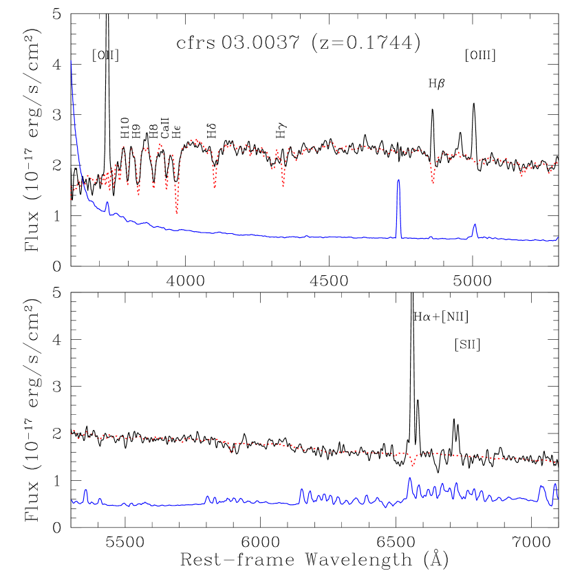
Figure 3: Example of input spectrum for the CFRS 03.0037 galaxy at $z=0.1744$. The solid line shows the observed spectrum, the blue line the error spectrum (magnified 5 times) and the red dotted line shows the continuum fitting.

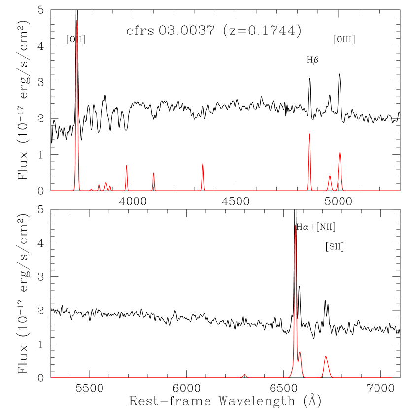
Figure 4: Example of emission-line fits, done after the continuum subtraction for the CFRS 03.0037 galaxy at $z=0.1744$.

4.1.2 Model templates

The template spectra used to fit the continuum emission of the galaxy in platefit were produced using the Bruzual & Charlot (2003) population synthesis model. At wavelengths between 3200 and 9500 Å, the template spectra rely on the STELIB stellar spectral library (Le Borgne et al. 2003), for which the resolution is about 3 Å FWHM.

The template spectra were chosen in order to represent, through non-negative linear combinations, the properties of galaxies with any star formation history and metallicity. Specifically, the spectra were selected to provide good coverage of SDSS-DR1 galaxies in the plane defined by the 4000 Å break and the H$\delta$ stellar absorption line strength, which are good indicators of the star formation history of a galaxy (e.g., Kauffmann et al. 2003b). The library includes 10 template spectra for each of the three metallicities $Z=0.2\,Z_{\odot}$, $Z_{\odot}$ and $2.5\,Z_{\odot}$. The spectra correspond to 10 instantaneous-burst models with ages of 0.005, 0.025, 0.10, 0.29, 0.64, 0.90, 1.4, 2.5, 5, and 11 Gyr.

4.2 Adaptation to non-SDSS spectra and measurement of emission lines

We have created an interface procedure which facilitates the analysis of our non-SDSS spectra with the platefit routines. The input spectra are provided as two FITS files each: one for the spectrum itself and another one for the error spectrum, the output spectra are written into ASCII files and the measurements are provided in a FITS table. The behaviour of the interface procedure is controlled by a parameter file which is an extension of that used in the platefit code and which controls the operation of the code.

The result of flux and equivalent-width measurements of the main emission lines is shown in Table References and in Table References.

4.2.1 Comparison with manual determination

It is instructive to compare the performance of the automatic fitting code with manual measurements of line fluxes using standard methods. To this end we measured emission lines from a subsample of the spectra using the task splot in IRAF. This subsample is made of the 31 first reduced spectra, that do not show any specific properties, among the CFRS sub-sample (see Table 1). In this section we will compare these manual results to the automatically computed ones. We expect to see significant differences for the Balmer lines where it is difficult to adjust for the contribution of the underlying stellar absorption when doing manual fitting. In contrast the measurements for the forbidden lines should be consistent within the errors as the effects of absorption lines for these is much less.

In Figure 5, we compare the automatic (using platefit) and manual measurements (using IRAF task splot) of oxygen emission-line equivalent widths (top panels) and fluxes (bottom panels). Figure 5 shows that there is a very good agreement between manual and automatic measurements for two of the strongest emission lines: [Oii]$\lambda$3727 and [Oiii]$\lambda$5007. Almost every point fall on the $y=x$ line and we also remark that the error estimates are consistent between the two methods. By comparing the bottom to the top panels, we see that the agreement is good both for equivalent-width or for line-flux measurements.

In Figure 6, we now compare the automatic and manual measurements of equivalent widths for Balmer emission lines (top panels) and low-intensity forbidden emission lines ([Nii]$\lambda$6584 and [Sii]$\lambda$6717, bottom panels). Figure 6 shows clearly the need to use platefit in order to have a good estimate of the Balmer emission lines. As we see in the top-left panel, manual measurements significantly underestimate the flux in the H$\beta$ emission line where underlying stellar absorption is normally not negligible in our galaxies. We note however that the difference between manual and automatic measurements for the H$\alpha$ emission line is smaller, which is to be expected since the underlying absorption is similar to that at H$\beta$, but the emission flux is considerably higher. The bottom panels show the same comparison for the fainter [Nii]$\lambda$6584 and [Sii]$\lambda$6717 emission lines. The dispersion here is larger but the measurements are consistent within the errors.

Two features are based on two blended emission lines each at our working resolution: the doublet [Sii]$\lambda\lambda$6717+6731 and the line ratio [Nii]$\lambda$6584/H$\alpha$. In Figure 7, we compare the automatic and manual measurements of these blended features (EWs: top panels, fluxes: bottom panels). Figure 7 illustrates the performance of platefit in deblending these lines. We see that platefit is able to give good results for the measurement of these low-intensity blended emission lines. To reach this level of accuracy we had to modify the way the equivalent width was estimated by platefit, which was optimised for higher resolution spectra. We tested various methods, and found that the best results were obtained when we calculated the equivalent width taking the continuum from the smoothed continuum spectra and combined this with the emission line flux. This allows us to make use of the line information in other parts of the spectrum to overcome the blending problems and we get a very good agreement between the measurements at different spectral resolutions as we will see below.

Figure 5: Comparison between oxygen emission lines measured automatically (using platefit) and manually (using IRAF task splot). Top panels: [Oii]$\lambda$3727 (left) and [Oiii]$\lambda$5007 (right) equivalent widths (in Å) given by platefit as a function of the manual measurement. Bottom panels: same for the measurements of line fluxes (in $10^{-17}$ erg s^-1 cm^-2). The solid line is the $x=y$ line and the dashed line is the linear regression.

Figure 6: Comparison between equivalent widths (in Å) for the Balmer (top panels) and [Nii]$\lambda$6584, [Sii]$\lambda$6717 (bottom panels) emission lines measured automatically (using platefit) and manually (using IRAF task splot). The solid line is the $x=y$ line and the dashed line is the linear regression.

Figure 7: Comparison between blended features computed from equivalent width (in Å, top panels) and from fluxes (in $10^{-17}$ erg s^-1 cm^-2, bottom panels) automatically (using platefit) and manually (using IRAF task splot): the line sum [Sii]$\lambda\lambda$6717+6731 (left) and the line ratio [Nii]$\lambda$6584/H$\alpha$ (right). The solid line is the $x=y$ line and the dashed line is the linear regression.

4.2.2 Resolution accuracy

To prepare for the spectral analysis of upcoming deep surveys, such as VVDS, we have used our medium resolution data to test the behaviour of platefit when used on spectra with a lower resolution. This point will be critical in particular for the [Nii]$\lambda$6584/H$\alpha$ ratio, as these two lines are blended in low-resolution spectra ($R_{\mathrm{s}}\lesssim 313$). The main issue is to determine if we can use this ratio to perform any spectral classification (see Sect. 6) and metallicity estimate (van Zee et al. 1998; Pettini & Pagel 2004). Our sample is approximatively at the spectral resolution $R_{\mathrm{s}}=500$, while the resolution of the VVDS is $R_{\mathrm{s}}=250$. Thus, we have downgraded the resolution of our spectra by a factor of two with a gaussian convolution, and we have rerun platefit on the new spectra.

Table 5 shows the difference between downgraded resolution and original resolution measurements for some characteristic lines. We see that the rms of the relative difference is low and strictly less than the error associated on each line. We also remark that there are some systematic shifts (i.e. the mean value of the difference is not null) but they are still lower than the error. Figure 8 shows that there is no dependence with the line intensity. For low resolution spectra, we reach a higher level of accuracy by tiding up the velocity dispersion of all the emission lines together, whatever they are forbidden or Balmer lines. This implies the assumption that all broad-line AGNs have been taken out of the sample before running the platefit software (see Sect. 6 below for a detailed discussion about the various spectral types of emission-line galaxies).

The [Nii]$\lambda$6584/H$\alpha$ line ratio as measured on the downgraded spectra is compared to the original measurements in Fig. 9 (see also Table 5). It is clear that the difference is small and consistent with zero within the errors. The logarithm of this line ratio, which is used for metallicity estimates, also has a weak dependence on the spectral resolution, and the scatter is lower than the standard error on metallicity calibrations ($\sim 0.2$ dex).

Table 5: Calculations of the mean and the rms of the difference between downgraded resolution and original resolution measurements. We give first the absolute values, and then the relative values which are more physically significant in percent (rel. columns). We compare these results to the mean of the error on the original data (two last columns).

parameter	mean	rel.	rms	rel.	err	rel.
EW([Oii]$\lambda$3727)	$-0.30$Å	$3.3$%	$2.09$Å	$9.8$%	$1.21$Å	$8.2$%
EW(H$\alpha$)	$+0.51$Å	$0.5$%	$3.32$Å	$9.0$%	$1.95$Å	$9.2$%
EW([Nii]$\lambda$6584)	$+0.69$Å	$12$%	$1.92$Å	$24$%	$1.93$Å	$47$%
[Nii]$\lambda$6584/H$\alpha$	$-0.02$	$11$%	$0.05$	$23$%	$0.05$	$47$%
log([Nii]$\lambda$6584/H$\alpha$)	$-0.06$ dex	$8.2$%	$0.12$ dex	$16$%	$0.20$ dex	$21$%

Figure 8: Comparison between the equivalent width (in Å) of [Oii]$\lambda$3727 (top-left), H$\alpha$ (top-right), H$\beta$ (bottom-left) and [Nii]$\lambda$6584 (bottom-right) measured at downgraded ($R_{\mathrm{s}}=250$) and original ($R_{\mathrm{s}}=500$) resolutions. The solid line is the $x=y$ line and the dashed line is the linear regression.

Figure 9: Comparison between the [Nii]$\lambda$6584/H$\alpha$ line ratio calculated with the equivalent widths measured at downgraded ($R_{\mathrm{s}}=250$) and original ($R_{\mathrm{s}}=500$) resolutions. The solid line is the $x=y$ line and the dashed line is the linear regression.

5 Photometric analysis

5.1 Photometric data

We measured the photometric magnitudes with SExtractor (Bertin & Arnouts 1996) in the $R$ band using the pre-imaging data. We used an input file with all the image coordinates of the galaxies and we computed the photometric magnitudes using the best radial adjustment (MAG_BEST parameter). We adopt these measurements in place of those from the literature for the CFRS sub-sample to ensure consistency with the CLUST sub-sample.

For the CFRS sub-sample, the pre-imaging was performed in the Gunn $R$ band with the VLT/FORS1 camera. For the CLUST sub-sample, pre-images have been acquired in the Bessel $R$ band with the FORS1 camera, except for the J1206 field, for which the pre-imaging has been done with the TEK2048 camera on the UH88in telescope in the $R$ band. For the LRIS data, we used observations of Abell 963, Abell 2218, Abell 2390 with the CFH12k camera at CFHT (Czoske et al. 2002) in the $I$ band. For the cluster Clg 1358+62, we measured photometry on an HST-WFPC image in the $F606W$ band.

The photometric calibration was performed in different ways depending on the field. The J1206 field was already calibrated. The other fields from the CLUST sub-sample were calibrated using a photometric standard star. For the CFRS sub-sample, the standard star was observed in a different filter than the galaxies (Bessel $R$ rather than Gunn $R$), preventing us from using it to do the calibration. Fortunately we were able to take advantage of the previously measured magnitudes of the CFRS galaxies in the $I$ band (CFHT FOCAM camera): the Bessel $R$ magnitudes of these objects were computed using spectroscopic colors (see Sect. 5.2), and we calculated the zero-point of each image by doing a linear regression.

The photometric magnitudes of the GDDS sub-sample were directly taken from the literature (Chen et al. 2002): $R$ band photometry of the NTT Deep field has been taken with the BTC camera on the Cerro Tololo Inter-American Observatory (CTIO) 4m telescope, $I$ band photometry of the NOAO-Cetus and SA22 fields have been taken with the CFH12k camera on the Canada France Hawaii Telescope (CFHT).

5.2 Spectroscopic magnitudes

We want to compute spectroscopic magnitudes, by integrating the flux through a set of filter response curves, in order to have information on the color (we only have photometric magnitudes in the $R$ band), on the $k$-correction and on the aperture differences (i.e. the amount of flux lost because of the limited size of the slits during spectroscopic observations) of our galaxies.

We used an adaptation of the filter_thru routine from the SDSS IDL library. For a flux-calibrated spectrum this routine returns a spectroscopic magnitude in the $AB$ system (Oke 1974). If the spectrum does not cover the full bandwidth of the filter (borders at 5%), it returns nothing. We computed spectroscopic magnitudes directly from the observed spectrum if it covers the full bandwidth of the filter, otherwise from the model spectrum given by the continuum fitting.

We used the filter response curve of the FORS1 camera (CCD + atmosphere) for the following bands: Bessel $B$, $V$, $R$ and $I$. We also have the filter response of the FORS1 camera in the Gunn $R$ band (used for the pre-imaging of the CFRS fields), of the TEK2048 camera in the $R$ band (used for the pre-imaging of the J1206 field), of the CFHT FOCAM camera in the $I$ band (used for the original CFRS data), and of the BTC camera in the $R$ band and the CFH12k camera in the $I$ band (used for the photometry of the GDDS sub-sample). Finally we also calculated the photometry in the $u$, $g$, $r$, and $i$ color system of the SDSS for possible comparison (Fukugita et al. 1996). We have checked that the spectroscopic colors are in good agreement (i.e. within the error bars) with published photometric colors.

We can use the information of the continuum SNR from Tables 1 and 2 to have an estimate of the uncertainties of the spectroscopic magnitudes. We use the following formula:

$$\Delta m\approx\frac{2.5}{\ln 10}\mathrm{SNR}^{-1}$$

We find a mean uncertainty of $\sim 0.1$ magnitudes.

5.3 Absolute magnitudes

The absolute magnitudes were computed using photometric magnitudes and the $k$-correction given from spectroscopic magnitudes (see Sect. 5.2). If we want, for example, the absolute magnitude in the $I$ band ($M_{\mathrm{AB}}(I)$) given a photometric magnitude in the $R$ band ($R_{\mathrm{AB}}$), we use the following formula:

$$M_{\mathrm{AB}}(I)=d+R_{\mathrm{AB}}+\left(I_{\mathrm{spec}}^{\mathrm{rest}}-R_{\mathrm{spec}}^{\mathrm{obs}}\right)$$

where $d$ is the distance modulus, $I_{\mathrm{spec}}^{\mathrm{rest}}$ and $R_{\mathrm{spec}}^{\mathrm{obs}}$ are the spectroscopic magnitudes computed respectively in rest-frame and in observed-frame so that $I_{\mathrm{spec}}^{\mathrm{rest}}-R_{\mathrm{spec}}^{\mathrm{obs}}$ is the $k$-correction. Note that we can alternatively write:

$$M_{\mathrm{AB}}(I)=d+I_{\mathrm{spec}}^{\mathrm{rest}}+\left(R_{\mathrm{AB}}-R_{\mathrm{spec}}^{\mathrm{obs}}\right)$$

where $R_{\mathrm{AB}}-R_{\mathrm{spec}}^{\mathrm{obs}}$ is the aperture difference. We remark that the aperture difference (ape in Table References) is less than $-1.3$ mag for a large majority of our sample, which means that the aperture coverage is at least $30$% of the galaxy total luminosity. This avoids important disk/bulge effects (see Kewley et al. 2005 for details). The distance modulus is calculated using the last cosmology given by WMAP (Spergel et al. 2003): $H_{\mathrm{0}}=71$ km s^-1 Mpc^-1, $\Omega_{\Lambda}=0.73$ and $\Omega_{\mathrm{m}}=0.27$. The following formula gives the distance modulus as a function of the redshift $z$:

$$d=-5\log\left(\frac{c}{H_{\mathrm{0}}\cdot 10\textrm{pc}}\cdot(1+z)\cdot\int_{0}^{z}f(z^{\prime})^{-1/2}dz^{\prime}\right)$$

where $f(z^{\prime})=(1+z^{\prime})^{2}(1+\Omega_{\mathrm{m}}z^{\prime})-\Omega_{\Lambda}z^{\prime}(2+z^{\prime})$.

The photometric magnitudes ($R_{AB}$ and $I_{AB}^{0}$ in Table References) are not corrected for foreground extinction whereas this is necessary for future scientific analysis. We thus take into account the foreground dust extinction from the Milky Way by using the Schlegel et al. (1998) dust maps ($A_{I}$ in Table References) for computing the rest-frame colors and the absolute magnitude.

5.4 Lensing corrections

For the galaxies in the CLUST sub-sample, we need to correct for the magnification effect caused by the gravitational lensing of the cluster. We do this using the most recent mass models for the galaxy clusters in this sample (for AC 114: Natarajan et al. 1998; Campusano et al. 2001; for Abell 2390: Pelló et al. 1999; for Cl 2244: Kneib et al., unpublished; for Abell 2218: Kneib et al. 1996; Ellis et al. 2001; for Abell 963: Smith et al. 2003; for Clg 1358:Franx et al. 1997). We derived the magnification at the redshift of our background sources with the LENSTOOL software developed by Kneib (1993). The corrections due to the lensing are usually small ($<0.3$ mags) compared with the photometric errors. For sources very close to the mean redshift of the cluster (for example in J 1206) no correction was applied.

The results are provided in Table References. The $I$-band absolute magnitude is given after correction for the foreground dust extinction, the $k$-correction and the lensing effect. We calculate the absolute magnitude in any others bands using the given spectroscopic colors.

5.5 Color-color diagrams

To gain some insight into the nature of the galaxy population in our sample, we start by constructing the $g-r$ versus $u-g$ color-color diagram (see Fig. 10). Strateva et al. (2001) has shown that this diagram separates galaxies into early and late types. We expect to see irregulars with a blue continuum at low $u-g$ and $g-r$ colors, whereas ellipticals, which have a substantial Balmer break, should have “red” $u-g$ and $g-r$ colours. To ease interpretation we use rest-frame colours throughout.

Figure 10 shows that our galaxy sub-samples are well distributed within the late-type region showing mainly irregular or Sc “color” types. The proportion of early-type spirals is much less and we have only a few ellipticals. This figure thus indicates that the latest spectral types are more likely to be observed, as confirmed by the histogram shown in Fig. 11. This result is primarily due to our selection criterion as we biased our sample in favor of emission-line galaxies. Indeed irregular galaxies usually have brighter emission lines than Sb galaxies, so they will be in our sample down to very low SNR. In contrast galaxies of (spectral) type Sb will only be included in our sample when their spectrum is of good SNR. Any possible effect introduced by this bias will have to be taken into account in subsequent analysis.

We must however remark that neither Fig. 10 nor Fig. 11 are accurate enough to determine which galaxy is of a given spectral type because of the high dispersion of the $u-r$ values for each spectral type (e.g. the effect of internal dust on the colors).

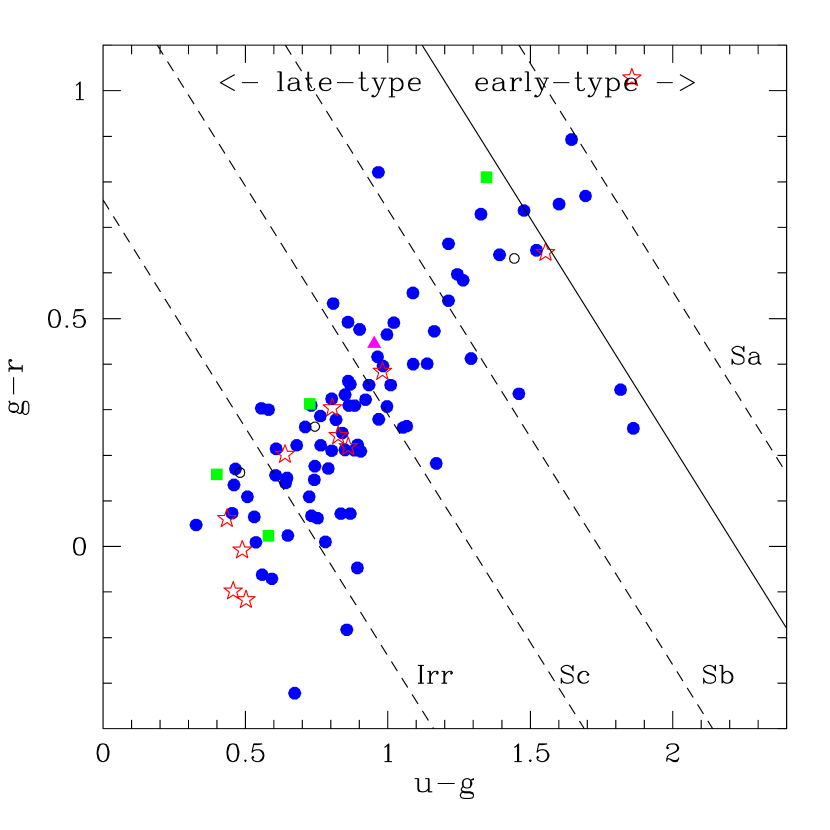
Figure 10: Rest-frame color-color diagram using SDSS passbands. The solid line shows the empirical separation ($u-r=2.22$) between late-type (below the line) and early-type (above the line) galaxies from Strateva et al. (2001). The dotted lines shows the mean value of the $u-r$ parameter for standard spectra of the Sa, Sb, Sc and Irr spectral types: respectively 2.56, 1.74, 1.29 and 0.76 (Strateva et al. 2001). The different symbols indicate star-forming galaxies and AGNs as determined in Sect. 6 (see the description of the symbols in Fig. 14).

Figure 11: Histogram of the rest-frame $u-r$ color. We plot the number of galaxies per 0.1 bin of the $u-r$ as an indicator of the spectral type. The solid and dotted lines are the same as in Fig. 10.

6 Spectral classification

6.1 Nature of the main ionizing source

As we want to focus the scientific analysis on star-forming galaxies, we have to make the difference between starbursts and AGNs which both show emission lines in their spectrum. The AGN population can be divided into three main types: Seyfert 1, Seyfert 2 and LINERs. The Seyfert 1, also called broad-line AGNs, can be excluded from our sample by comparing the FWHM of the Balmer emission lines to the FWHM of the forbidden lines: those galaxies with a significantly higher FWHM for the Balmer lines are expected to be Seyfert 1. The ratio of the FWHM of the Balmer lines to that of the forbidden lines is consistent with unity for most of our sample galaxies (mean of $0.98$ with a rms scatter of $0.18$). We found 6 peculiar objects showing Balmer lines significantly broader than forbidden ones ($FWHM_{\mathrm{Balmer}}/FWHM_{\mathrm{forbidden}}\sim 2-3$). These objects could be classified as Seyfert 1 galaxies. However, after a careful visual inspection of individual spectra, we found that the measurement of the FWHM of the Balmer lines in these galaxies is disrupted by either weak Balmer emission lines or noise features. These objects are thus classified as narrow emission-line galaxies.

6.2 Diagnostic diagrams

6.2.1 “Red” diagnostics diagrams

We still need to separate star-forming galaxies from narrow-line AGNs, namely Seyfert 2 and LINERs. Seyfert 2 have a high excitation degree compared to LINERs. The standard prescription (Veilleux & Osterbrock 1987) makes use of the [Nii]$\lambda$6584/H$\alpha$, [Sii]$\lambda\lambda$6717+6731/H$\alpha$ and [Oiii]$\lambda$5007/H$\beta$ line ratios to separate the star-forming galaxies from AGNs; and the [Oiii]$\lambda$5007/H$\beta$ as an indicator of the ionization level to distinguish Seyfert 2 from LINERs.

The standard diagnostic diagrams are shown in Fig. 12 for the [Nii] diagnostic and in Fig. 13 for the [Sii] diagnostic. The limit between star-forming galaxies and AGNs are given by Kewley et al. (2001) (+ 0.15dex for the [Sii] diagnostic in order to take into account the model uncertainties). The star-forming galaxies are well separated from AGNs and follow a clear sequence covering a large range of ionization levels and collisional excitation degrees. The classification is obvious, i.e. the [Nii] and [Sii] diagnostics are in agreement, for 37 galaxies: 34 are star-forming galaxies and 3 are Seyfert 2.

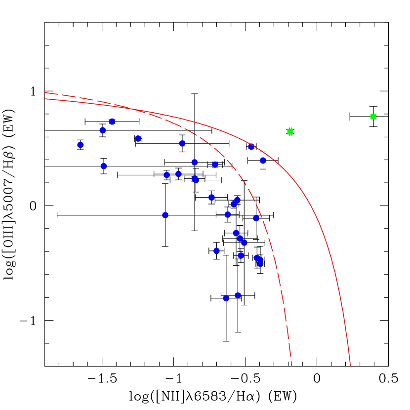
Figure 12: Standard diagnostic diagram using the [Nii]$\lambda$6584/H$\alpha$ emission-line ratio. Blue circles identify star-forming galaxies, green squares indicate AGNs (Seyfert 2) and magenta triangles show contradictory cases (see text for details). The solid line shows the theoretical limit from Kewley et al. (2001). The dashed line is the empirical limit from Kauffmann et al. (2003a) for SDSS galaxies.

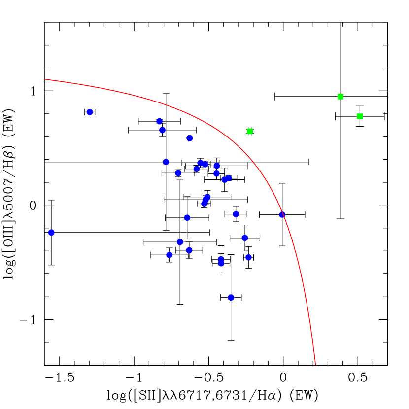
Figure 13: Standard diagnostic diagram using the [Sii]$\lambda\lambda$6717+6731/H$\alpha$ emission-line ratio. Same legend as in Fig. 12.

6.2.2 “Blue” diagnostic diagrams

As recently pointed by Lamareille et al. (2004), we can also use the “blue” emission lines (i.e. [Oii]$\lambda$3727, [Oiii]$\lambda$5007 and H$\beta$) to perform the spectral classification for higher redshift galaxies (i.e. with no observable H$\alpha$ and [Nii]$\lambda$6584 “red” lines) but with a lower accuracy. We note that 104 galaxies (73.8% of our sample) can only be classified with the blue diagnostics. The blue diagnostic diagrams are shown in Fig. 14 and in Fig. 15. Please note that we use theses diagrams without any correction for dust extinction (as calibrated on 2dFGRS data), by the use of equivalent widths instead of fluxes (see Sect. 6.2.3 below).

We found four objects (LCL05 045, LCL05 065, LCL05 109, and LCL05 142), very close in the $R_{\mathrm{23}}$ vs. $O_{\mathrm{32}}$ classification (four points on top of Fig. 15), which are classified as Seyfert 2 according to this diagram. However this classification is not in agreement with i) the “red” classification as star-forming galaxy that we derive for one of them (LCL05 065), ii) with the overall aspect of their spectra (very faint continuum and high ionization state typical of HII galaxies), or with the low [Nii]/H$\alpha$ ratio estimated recently from NIR spectroscopy for LCL05 045 (Maier:2005astro.ph..8239M). We conclude that the $R_{\mathrm{23}}$ vs. $O_{\mathrm{32}}$ “blue” classification, calibrated on the 2dFGRS data, may not be valid on its upper part. For these four objects, we keep only the results from the [Oiii]$\lambda$5007/H$\beta$ vs. [Oii]$\lambda$3727/H$\beta$ classification, i.e. candidate star-forming galaxies (see below).

We found four objects (LCL05 017, LCL05 097, LCL05 115, and LCL05 130) which are classified as Seyfert 2 galaxies but with very high error bars on the diagnostic diagrams. These objects show noisy spectra and/or undetected H$\beta$ emission line (while oxygen lines are detected). Therefore their classification as Seyfert 2 is not fully secure.

We have a number of objects which fall into the error domain on the two “blue” diagrams and are thus unclassified. After checking their spectra, we decided to keep them in our sample as candidate star-forming galaxies, keeping in mind in the subsequent analysis that their emission-line spectrum could be contaminated by a low-luminosity AGN.

We finally find 115 (81.6%) “secure” star-forming galaxies, 7 (5.0%) Seyfert 2, 16 (11.3%) “candidate” star-forming galaxies, and 3 (2.1%) objects which are still unclassified (i.e. they have one or more missing lines). Results are shown in Table References.

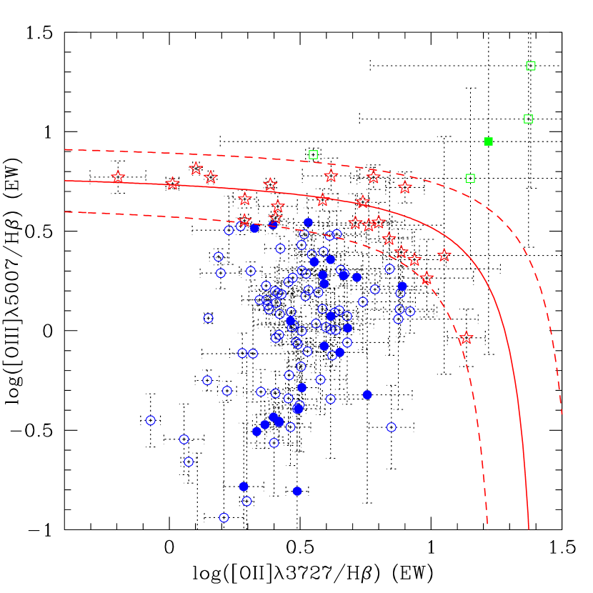
Figure 14: “Blue” diagnostic diagram. The symbols show the results of the “blue” diagnostic: blue circles for star-forming galaxies, green squares for AGNs (Seyfert 2), magenta triangles for contradictory cases and red stars for unclassified objects. Filled symbols are for objects already classified with standard diagnostic diagrams. The solid line shows the empirical calibration from Lamareille et al. (2004) and the dashed lines the associated error domain.

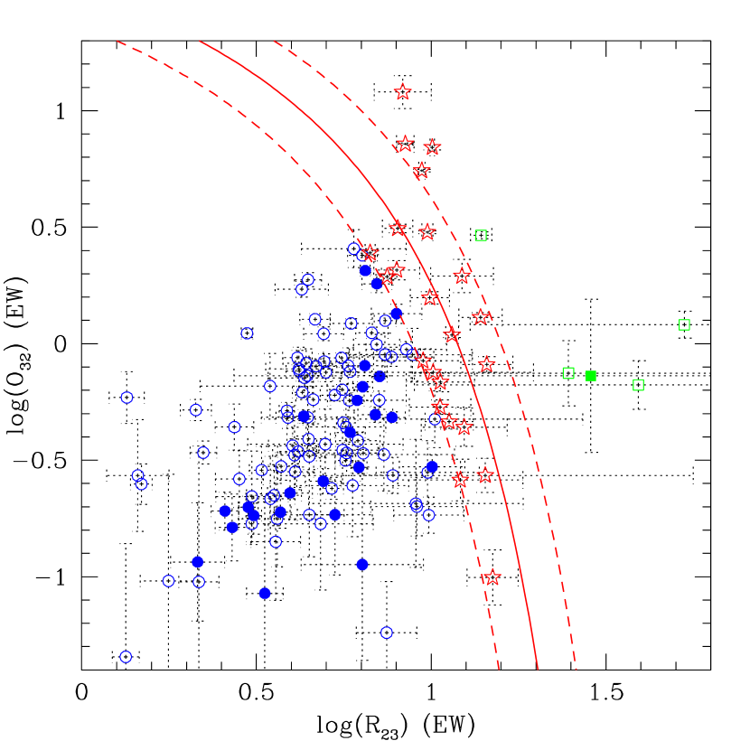
Figure 15: Another “blue” diagnostic diagram. Same legend as in Fig. 14.

6.2.3 Discussion on dust extinction

The “red” diagnostic diagram makes use of various line ratios which are all insensitive to the dust extinction because they involve emission lines with similar wavelengths ([Nii]$\lambda$6548, [Sii]$\lambda\lambda$6717,6731 and H$\alpha$ in one case, [Oiii]$\lambda\lambda$4959,5007 and H$\beta$ in the other case). This is not the case for the “blue” diagnostic diagrams which make use of the [Oii]$\lambda$3727 and H$\beta$ emission lines in the same ratio. These diagrams can then be strongly affected by the dust extinction.

The effect of dust is minimized by the use of equivalent width measurements instead of fluxes. Indeed no correction for reddening is needed on equivalent width ratios, if we assume that the attenuation in the continuum and emission lines is the same. To check this assumption, we have derived dust extinction values from the observed H$\alpha$/H$\beta$ Balmer decrement on the $24$ galaxies where it is possible (we use the extinction law of Seaton 1979, and a theoretical Balmer decrement of $2.87$ from Osterbrock 1989). The E($B-V$) coefficients that we found are given in Table References. We then used these results to correct the [Oii]$\lambda$3727/H$\beta$ flux ratio for reddening and we compared it to the same equivalent width ratio.

Fig. 16 shows the result of this comparison. We see that the equivalent width ratio is consistent with the dust-corrected flux ratio, with the exception of two very high ratios which are underestimated with equivalent widths. The rms of the residuals around the $y=x$ line is $0.10$ dex. We conclude that the “blue” diagnostic diagrams are not significantly affected by the differential attenuation between [Oii]$\lambda$3727 and H$\beta$ emission lines. The low value of the rms of the residuals tells us that any possible effect is already included in the error domain of the “blue” calibration.

Figure 16: Comparison between the equivalent-width ($x$-axis) and dust-corrected flux ($y$-axis) ratio of [Oii]$\lambda$3727 and H$\beta$ emission lines. The solid line shows the $y=x$ curve and the dashed line is the fit to the data.

7 Conclusions

We have defined a sample of 141 emission-line galaxies at intermediate redshifts ranging from $z=0.2$ to $z=1.0$. We obtained medium-resolution spectroscopic observations of these galaxies in the optical range, and associated $R$-band photometry. The following conclusions can be drawn from this paper:

• Our sample has been used to test the platefit software originally developed by C. Tremonti, and which is designed to automatically measure spectral features (e.g. emission lines). We managed to adapt it to our lower resolution and SNR spectra. The comparison with manual measurements shows that we get better measurements for those emission lines where Balmer absorption features are important (e.g. H$\alpha$, H$\beta$ and [Oii]$\lambda$3727 emission lines), and that we get correct measurements of flux and equivalent widths for blended lines (e.g. [Nii]$\lambda$6584 and H$\alpha$ emission lines).

• We have done as careful a job as possible and are reasonably sure that the platefit software can also be used for future and ongoing large surveys (VVDS, zCOSMOS, etc) which are based on low resolution spectroscopy. We verify, by downgrading the resolution of our spectra, that the flux and equivalent-width measurements at low resolution are not altered more than the measurement error. In particular, the [Nii]$\lambda$6584/H$\alpha$ line ratio is robust to resolution changes.

• The platefit software has been used to measure $k$-corrected spectroscopic colors. Our sample of galaxies covers all the late-type range in a color-color diagram, with a maximum for the Irregular and Sc spectral types.

• Standard and “blue” diagnostic diagrams show a majority of star-forming galaxies, and some narrow-lines AGNs (i.e. Seyfert 2 galaxies), covering the whole range of ionization level and collisional excitation degree. Because the H$\alpha$ line gets redshifted out of the optical range at high redshifts, $\sim$ 70% of our sample must be classified using the “blue” diagnostic diagrams. About 10% of our galaxies still remain unclassified because they fall in the uncertainty region of these diagrams, we classify them as “candidate” star-forming galaxies.

More analysis in terms of chemical abundances and stellar populations will be described in subsequent papers.

[x]lrrrrrrrrrrrrrr Photometric data. LCL05: identification number, see Tables 1, 2 and 3.$R_{\mathrm{AB}}$: photometric magnitude in the $R$ band (or $I$ band for filter 5). filter: the filter used (1: FORS $R$ Gunn, 2: FORS $R$ Bessel, 3: TEK2048 $R$, 4: BTC $R$, 5: CFH12k $I$, 6: WFPC $F606W$). ape: aperture differences (the difference between observed and spectroscopic magnitude in the given filter). $I_{\mathrm{AB}}^{0}$: $k$-corrected magnitude in the $I$ band (the sum of the spectroscopic magnitude in rest-frame and the aperture differences). $A_{I}$: foreground dust extinction in the $I$ band (rest-frame). $(U-B)_{\mathrm{AB}}^{0}$,$(B-V)_{\mathrm{AB}}^{0}$, $(V-R)_{\mathrm{AB}}^{0}$, $(V-I)_{\mathrm{AB}}^{0}$: foreground-dust- and $k$-corrected spectroscopic colors. $(u-g)_{\mathrm{AB}}^{0}$,$(g-r)_{\mathrm{AB}}^{0}$, $(g-i)_{\mathrm{AB}}^{0}$: foreground-dust- and $k$-corrected spectroscopic colors with the SDSS filters. $M_{\mathrm{AB}}(I)$: foreground-dust- and $k$-corrected absolute magnitude in the $I$ band. lens: lensing correction if necessary (already applied to $M_{\mathrm{AB}}(I)$).
LCL05 $R_{\mathrm{AB}}$ filter ape $I_{\mathrm{AB}}^{0}$ $A_{I}$ $(U-B)_{\mathrm{AB}}^{0}$ $(B-V)_{\mathrm{AB}}^{0}$ $(V-R)_{\mathrm{AB}}^{0}$ $(V-I)_{\mathrm{AB}}^{0}$ $(u-g)_{\mathrm{AB}}^{0}$ $(g-r)_{\mathrm{AB}}^{0}$ $(g-i)_{\mathrm{AB}}^{0}$ $M_{\mathrm{AB}}(I)$ lens
continued.
LCL05 $R_{\mathrm{AB}}$ filter ape $I_{\mathrm{AB}}^{0}$ $A_{I}$ $(U-B)_{\mathrm{AB}}^{0}$ $(B-V)_{\mathrm{AB}}^{0}$ $(V-R)_{\mathrm{AB}}^{0}$ $(V-I)_{\mathrm{AB}}^{0}$ $(u-g)_{\mathrm{AB}}^{0}$ $(g-r)_{\mathrm{AB}}^{0}$ $(g-i)_{\mathrm{AB}}^{0}$ $M_{\mathrm{AB}}(I)$ lens
001 $21.22$ 1 $-0.56$ $21.03$ $0.04$ … $0.49$ $0.17$ $0.31$ $0.88$ $0.31$ $0.46$ $-20.26\pm 0.04$ $0.00$
002 $21.11$ 1 $-0.54$ $21.26$ $0.02$ $1.01$ $0.21$ $0.00$ $-0.01$ $0.89$ $-0.05$ $-0.07$ $-21.56\pm 0.04$ $0.00$
003 $20.47$ 1 $-0.61$ $20.37$ $0.04$ $1.20$ $0.31$ $0.16$ $0.32$ $0.68$ $0.22$ $0.38$ $-20.93\pm 0.03$ $0.00$
004 $19.92$ 1 $-1.41$ $19.43$ $0.04$ $0.83$ $0.36$ $0.28$ $0.62$ … $0.41$ $0.69$ $-21.27\pm 0.02$ $0.00$
005 $19.19$ 1 $-0.63$ $18.68$ $0.04$ … $0.89$ $0.30$ $0.56$ … $0.63$ $0.92$ $-22.02\pm 0.01$ $0.00$
006 $21.14$ 1 $-0.69$ $20.96$ $-0.05$ $1.14$ $0.34$ $0.13$ $0.26$ $1.05$ $0.26$ $0.37$ $-19.45\pm 0.04$ $0.00$
007 $20.15$ 1 $-0.57$ $19.85$ $0.04$ $0.94$ $0.58$ $0.22$ $0.40$ … $0.47$ $0.65$ $-20.86\pm 0.02$ $0.00$
008 $20.87$ 1 $-0.61$ $20.71$ $0.04$ … $0.30$ $0.15$ $0.32$ … $0.30$ $0.41$ $-19.76\pm 0.03$ $0.00$
009 $20.22$ 1 $-0.59$ $20.04$ $0.04$ … $0.44$ $0.16$ $0.31$ … $0.34$ $0.48$ $-20.83\pm 0.02$ $0.00$
010 $20.88$ 1 $-0.60$ $20.24$ $0.04$ $1.27$ $0.83$ $0.38$ $0.68$ $1.48$ $0.74$ $1.03$ $-20.45\pm 0.03$ $0.00$
011 $20.48$ 1 $-1.09$ $20.26$ $0.04$ $1.21$ $0.36$ $0.20$ $0.38$ $0.85$ $0.33$ $0.49$ $-20.69\pm 0.03$ $0.00$
012 $20.95$ 1 $-0.79$ $20.54$ $0.05$ $3.93$ $0.83$ $0.33$ $0.61$ … $0.60$ $0.91$ $-17.49\pm 0.04$ $0.00$
013 $21.14$ 1 $-1.36$ $20.80$ $0.04$ $2.06$ $0.56$ $0.22$ $0.42$ $1.14$ $0.40$ $0.61$ $-19.71\pm 0.04$ $0.00$
014 $20.61$ 1 $-1.34$ $19.58$ $0.04$ $2.23$ $0.94$ $0.46$ $0.86$ $1.69$ $0.77$ $1.20$ $-22.07\pm 0.03$ $0.00$
015 $22.75$ 1 $-0.13$ $22.81$ $0.05$ $0.80$ $0.18$ $0.07$ $0.16$ $0.84$ $0.07$ $0.14$ $-17.65\pm 0.10$ $0.00$
016 $21.07$ 1 $-0.69$ $21.47$ $0.04$ $0.51$ $0.16$ $-0.08$ $0.04$ $0.59$ $-0.07$ $-0.05$ $-19.49\pm 0.03$ $0.00$
017 $21.01$ 1 $-1.11$ $20.46$ $0.04$ … $0.79$ $0.36$ $0.63$ … $0.65$ $0.96$ $-20.02\pm 0.04$ $0.00$
018 $21.22$ 1 $-0.81$ $21.01$ $0.13$ … $0.37$ $0.14$ $0.27$ … $0.28$ $0.39$ $-19.10\pm 0.05$ $0.00$
019 $22.11$ 1 $-0.65$ $23.00$ $0.14$ … … $-0.03$ $-0.86$ … $0.27$ $-0.24$ $-16.93\pm 0.12$ $0.00$
020 $21.95$ 1 $-0.53$ $21.53$ $0.11$ … $0.45$ $0.21$ $0.40$ $0.86$ $0.36$ $0.57$ $-20.72\pm 0.10$ $0.00$
021 $21.16$ 1 $-0.46$ $21.00$ $0.13$ … $0.48$ $0.23$ $0.37$ … $0.23$ $0.30$ $-19.71\pm 0.05$ $0.00$
022 $21.85$ 1 $-0.40$ $22.00$ $0.08$ $0.60$ $0.10$ $0.04$ $0.08$ $0.54$ $0.01$ $0.05$ $-20.83\pm 0.09$ $0.00$
023 $20.90$ 1 $-0.78$ $20.60$ $0.11$ $1.00$ $0.36$ $0.19$ $0.35$ $0.76$ $0.29$ $0.46$ $-21.58\pm 0.05$ $0.00$
024 $21.72$ 1 $-0.77$ $21.49$ $0.05$ … $0.26$ $0.12$ $0.24$ $0.61$ $0.16$ $0.28$ $-21.52\pm 0.09$ $0.00$
025 $20.73$ 1 $-1.44$ $20.54$ $0.15$ $1.17$ $0.29$ $0.15$ $0.29$ $0.86$ $0.22$ $0.37$ $-19.76\pm 0.06$ $0.00$
026 $21.63$ 1 $-0.87$ $21.19$ $0.15$ … $1.36$ $0.59$ $0.84$ … $0.10$ $0.36$ $-19.11\pm 0.08$ $0.00$
027 $22.42$ 1 $-0.85$ $22.37$ $0.13$ $1.13$ $0.31$ $0.01$ $0.13$ … $0.16$ $0.17$ $-17.91\pm 0.12$ $0.00$
028 $19.76$ 1 $-0.82$ $19.55$ $0.15$ $1.83$ $0.41$ $0.17$ $0.30$ $1.46$ $0.33$ $0.45$ $-20.21\pm 0.02$ $0.00$
029 $21.13$ 1 $-1.16$ $20.50$ $0.10$ $1.21$ $0.50$ $0.27$ $0.53$ $0.96$ $0.42$ $0.69$ $-21.92\pm 0.06$ $0.00$
030 $22.24$ 1 $-0.66$ $22.16$ $0.08$ $1.04$ $0.21$ $0.09$ $0.18$ $0.65$ $0.15$ $0.25$ $-20.69\pm 0.13$ $0.00$
031 $22.32$ 1 $-0.36$ $22.07$ $0.14$ … $0.34$ $0.13$ $0.30$ … $0.29$ $0.39$ $-18.23\pm 0.12$ $0.00$
032 $22.00$ 1 $0.09$ $21.55$ $0.07$ … $0.38$ $0.29$ $0.51$ … $-0.17$ $0.60$ $-20.61\pm 0.06$ $0.00$
033 $21.33$ 1 $-0.19$ $20.91$ $0.08$ $1.56$ $0.66$ $0.25$ $0.43$ $1.21$ $0.54$ $0.72$ $-20.06\pm 0.03$ $0.00$
034 $21.16$ 1 $-0.47$ $21.13$ $0.08$ … $0.53$ $0.24$ $0.31$ $0.73$ $0.07$ $0.14$ $-20.04\pm 0.03$ $0.00$
035 $21.16$ 1 $-0.50$ $21.03$ $0.09$ $1.50$ $0.26$ $0.17$ $0.30$ $0.80$ $0.21$ $0.35$ $-19.92\pm 0.03$ $0.00$
036 $21.05$ 1 $0.24$ $20.89$ $0.10$ $1.22$ $0.24$ $0.11$ $0.25$ $0.86$ $0.31$ $0.31$ $-19.26\pm 0.02$ $0.00$
037 $20.61$ 1 $-0.39$ $19.71$ $0.08$ … $0.49$ $0.56$ $0.97$ … $0.00$ $1.03$ $-22.16\pm 0.03$ $0.00$
038 $20.37$ 1 $-0.08$ $20.21$ $0.10$ … … $0.10$ $0.29$ … $0.23$ $0.32$ $-20.18\pm 0.02$ $0.00$
039 $20.45$ 1 $-0.57$ $20.31$ $0.08$ $1.24$ $0.36$ $0.14$ $0.27$ $1.07$ $0.26$ $0.38$ $-20.65\pm 0.02$ $0.00$
040 $21.51$ 1 $-0.49$ $21.59$ $0.06$ $1.19$ $0.18$ $0.08$ $0.16$ $0.53$ $0.07$ $0.15$ $-20.92\pm 0.04$ $0.00$
041 $20.66$ 1 $-2.75$ $20.13$ $0.09$ $2.20$ $0.60$ $0.39$ $0.69$ $1.82$ $0.34$ $0.87$ $-20.09\pm 0.03$ $0.00$
042 $22.17$ 1 $-1.05$ $22.28$ $0.08$ $1.07$ $0.18$ $0.10$ $0.21$ $0.45$ $0.07$ $0.18$ $-19.15\pm 0.08$ $0.00$
043 $22.49$ 1 $-0.46$ $21.92$ $0.09$ $0.77$ $0.56$ $0.27$ $0.57$ … $0.49$ $0.78$ $-19.30\pm 0.09$ $0.00$
044 $20.44$ 1 $-0.65$ $20.08$ $0.10$ $1.48$ $0.54$ $0.21$ $0.41$ $0.98$ $0.40$ $0.61$ $-20.75\pm 0.02$ $0.00$
045 $21.77$ 1 $-0.43$ $21.34$ $0.07$ $0.82$ $0.10$ $0.26$ $0.63$ $0.50$ $-0.12$ $0.25$ $-20.82\pm 0.04$ $0.00$
046 $22.26$ 1 $-0.20$ $21.65$ $0.04$ $1.24$ $0.45$ $0.21$ $0.41$ $0.87$ $0.36$ $0.56$ $-21.34\pm 0.08$ $0.00$
047 $23.42$ 1 $-0.39$ $22.95$ $0.07$ $0.96$ $0.28$ $0.27$ $0.59$ $0.56$ $0.30$ $0.64$ $-19.23\pm 0.25$ $0.00$
048 $22.11$ 1 $-1.07$ $21.97$ $0.09$ $0.97$ $0.29$ $0.11$ $0.29$ $0.74$ $0.26$ $0.35$ $-19.02\pm 0.08$ $0.00$
049 $20.62$ 1 $-0.53$ $20.11$ $0.10$ … $0.60$ $0.30$ $0.59$ … $0.56$ $0.81$ $-20.27\pm 0.02$ $0.00$
050 $22.15$ 1 $-0.65$ $21.25$ $0.05$ $1.19$ $0.56$ $0.37$ $0.72$ $0.86$ $0.49$ $0.87$ $-21.24\pm 0.09$ $0.00$
051 $21.66$ 1 $-0.56$ $21.74$ $0.08$ … $0.32$ $0.13$ $0.26$ $0.49$ $-0.01$ $0.13$ $-19.91\pm 0.05$ $0.00$
052 $21.57$ 1 $-0.14$ $21.77$ $0.08$ $0.95$ $0.36$ $-0.01$ $0.11$ $0.58$ $0.02$ $0.14$ $-19.08\pm 0.07$ $0.00$
053 $20.93$ 1 $-0.25$ $20.99$ $0.05$ $1.28$ $0.22$ $0.08$ $0.16$ $0.64$ $0.14$ $0.21$ $-21.51\pm 0.05$ $0.00$
054 $20.88$ 1 $-0.36$ $21.17$ $0.05$ $1.17$ $0.11$ $0.01$ $0.05$ $0.65$ $0.02$ $0.05$ $-21.35\pm 0.03$ $0.00$
055 $20.23$ 1 $-0.35$ $19.32$ $0.06$ … $0.97$ $0.33$ $0.64$ $1.24$ $0.60$ $0.93$ $-22.82\pm 0.02$ $0.00$
056 $19.89$ 1 $-0.59$ $19.24$ $0.08$ $1.70$ $0.78$ $0.37$ $0.67$ $1.39$ $0.64$ $0.96$ $-21.60\pm 0.02$ $0.00$
057 $19.67$ 1 $-0.19$ $18.82$ $0.08$ … $0.94$ $0.47$ $0.81$ $1.60$ $0.75$ $1.13$ $-22.46\pm 0.01$ $0.00$
058 $21.30$ 1 $-0.96$ $21.86$ $0.07$ $0.35$ $-0.34$ $-0.21$ $-0.41$ … $-0.49$ $-0.71$ $-19.09\pm 0.05$ $0.00$
059 $20.71$ 1 $-0.69$ $20.33$ $0.09$ $1.80$ $0.40$ $0.22$ $0.52$ $0.97$ $0.28$ $0.57$ $-20.50\pm 0.04$ $0.00$
060 $21.79$ 1 $-0.11$ $21.74$ $0.08$ $1.00$ $0.18$ $0.18$ $0.31$ $0.74$ $0.18$ $0.31$ $-19.73\pm 0.07$ $0.00$
061 $21.11$ 1 $-0.15$ $20.67$ $0.08$ $0.73$ $0.40$ $0.29$ $0.58$ $0.88$ $0.21$ $0.67$ $-20.80\pm 0.04$ $0.00$
062 $21.08$ 1 $-0.13$ $20.70$ $0.08$ $1.13$ $0.52$ $0.24$ $0.45$ $1.00$ $0.46$ $0.66$ $-20.19\pm 0.04$ $0.00$
063 $21.59$ 1 $-0.18$ $21.37$ $0.08$ … $0.13$ $0.33$ $0.51$ … $-0.31$ $0.43$ $-19.51\pm 0.05$ $0.00$
064 $20.56$ 2 $-0.77$ $19.60$ $0.15$ $1.90$ $0.99$ $0.53$ $0.98$ $1.35$ $0.81$ $1.31$ $-20.95\pm 0.01$ $0.00$
065 $21.88$ 2 $-0.76$ $21.64$ $0.21$ $0.92$ $0.45$ $-0.10$ $0.07$ $0.46$ $0.14$ $0.07$ $-15.93\pm 0.03$ $0.00$
066 $23.42$ 2 $-1.02$ $22.76$ $0.13$ … … $0.14$ $0.54$ $0.56$ $-0.06$ $0.29$ $-19.19\pm 0.15$ $0.01$
067 $22.48$ 2 $-0.71$ $22.92$ $0.11$ $1.60$ $0.13$ $-0.07$ $-0.15$ $0.86$ $-0.18$ $-0.27$ $-19.16\pm 0.07$ $0.01$
068 $22.95$ 2 $-0.91$ $22.37$ $0.05$ $1.13$ $0.30$ $0.19$ $0.50$ $0.74$ $0.15$ $0.44$ $-20.51\pm 0.13$ $0.03$
069 $21.42$ 2 $-1.68$ $21.23$ $0.17$ $1.59$ $0.42$ $0.15$ $0.27$ $0.73$ $0.31$ $0.36$ $-19.12\pm 0.03$ $0.00$
070 $22.73$ 2 $-0.06$ $21.73$ $0.03$ $1.13$ $0.36$ $0.29$ $0.78$ $0.58$ $0.30$ $0.77$ $-21.53\pm 0.12$ $0.06$
071 $21.72$ 2 $-0.90$ $21.64$ $0.10$ $0.91$ $0.19$ $0.12$ $0.23$ $0.51$ $0.11$ $0.23$ $-20.70\pm 0.03$ $0.15$
072 $21.99$ 2 $-0.98$ $21.82$ $0.13$ $1.53$ $0.38$ $0.13$ $0.25$ $0.85$ $0.21$ $0.34$ $-19.55\pm 0.03$ $0.04$
073 $20.59$ 2 $-0.94$ $20.49$ $0.02$ … $0.40$ $0.12$ $0.28$ … $0.31$ $0.43$ $-20.12\pm 0.01$ $0.00$
074 $19.21$ 2 $-2.03$ $19.20$ $0.03$ … … $0.53$ $0.61$ … $0.13$ $-0.04$ $-19.03\pm 0.00$ $0.00$
075 $20.34$ 2 $-1.53$ $20.26$ $0.03$ … … $0.07$ $0.21$ … $0.22$ $0.16$ $-18.02\pm 0.01$ $0.00$
076 $20.15$ 2 $-0.68$ $20.05$ $0.02$ $1.26$ $0.40$ $0.13$ $0.28$ … $0.28$ $0.43$ $-21.08\pm 0.01$ $0.00$
077 $20.28$ 2 $-0.49$ $20.20$ $0.02$ … $0.54$ $0.22$ $0.35$ $1.86$ $0.26$ $0.39$ $-20.76\pm 0.01$ $0.00$
078 $20.92$ 2 $-1.16$ $20.39$ $0.01$ $1.16$ $0.51$ $0.24$ $0.46$ $1.09$ $0.40$ $0.63$ $-21.93\pm 0.01$ $0.27$
079 $21.79$ 2 $-0.93$ $21.32$ $0.02$ $1.44$ $0.60$ $0.28$ $0.52$ $1.16$ $0.47$ $0.74$ $-20.28\pm 0.02$ $0.16$
080 $21.19$ 2 $-0.90$ $21.22$ $0.02$ … $0.85$ $0.22$ $0.32$ $1.17$ $0.18$ $0.28$ $-19.99\pm 0.01$ $0.00$
081 $23.47$ 2 $-0.28$ $23.29$ $0.02$ $0.70$ $0.27$ $0.24$ $0.43$ $0.79$ $0.17$ $0.46$ $-18.23\pm 0.05$ $0.04$
082 $20.25$ 2 $-0.97$ $19.55$ $0.02$ … $0.85$ $0.35$ $0.64$ $1.44$ $0.63$ $0.96$ $-22.15\pm 0.01$ $0.06$
083 $22.64$ 2 $-0.40$ $22.81$ $0.01$ $0.89$ $0.07$ $0.05$ $0.18$ $0.33$ $0.05$ $0.15$ $-20.30\pm 0.03$ $0.14$
084 $22.26$ 2 $-0.67$ $21.83$ $0.02$ $1.25$ $0.59$ $0.23$ $0.47$ $0.95$ $0.45$ $0.71$ $-19.89\pm 0.04$ $0.03$
085 $23.20$ 2 $-0.72$ $23.02$ $0.01$ $1.27$ $0.30$ $0.12$ $0.23$ $0.64$ $0.20$ $0.32$ $-20.12\pm 0.05$ $0.09$
086 $22.58$ 2 $-0.73$ $22.37$ $0.02$ $-2.15$ $-0.92$ $0.19$ $0.34$ $0.92$ $0.32$ $0.48$ $-19.36\pm 0.07$ $0.04$
087 $22.75$ 2 $-0.96$ $22.64$ $0.02$ $0.90$ $0.63$ $-0.10$ $0.09$ $0.61$ $0.21$ $0.41$ $-19.03\pm 0.04$ $0.07$
088 $23.22$ 2 $-0.62$ $23.39$ $0.00$ $0.97$ $0.10$ $0.04$ $0.09$ $0.43$ $0.06$ $0.11$ $-19.97\pm 0.09$ $0.00$
089 $22.14$ 2 $-0.70$ $21.87$ $0.04$ $1.14$ $0.41$ $0.15$ $0.27$ $0.83$ $0.24$ $0.37$ $-20.70\pm 0.03$ $0.04$
090 $22.37$ 2 $-0.88$ $21.91$ $0.04$ $1.07$ $0.43$ $0.23$ $0.44$ $0.80$ $0.30$ $0.53$ $-20.68\pm 0.04$ $0.03$
091 $22.30$ 2 $-0.87$ $21.77$ $0.04$ … $2.14$ $0.05$ $0.12$ $0.72$ $0.11$ $0.17$ $-21.66\pm 0.04$ $0.07$
092 $22.53$ 2 $-0.60$ $22.52$ $0.08$ $1.32$ $0.06$ $0.08$ $0.24$ $0.46$ $-0.10$ $0.05$ $-18.73\pm 0.04$ $0.00$
093 $22.15$ 2 $-1.05$ $21.96$ $0.03$ $1.20$ $0.21$ $0.14$ $0.34$ $0.46$ $0.17$ $0.36$ $-20.87\pm 0.03$ $0.10$
094 $23.63$ 2 $-0.30$ $23.60$ $0.06$ $1.28$ $0.23$ $0.11$ $0.20$ $0.48$ $0.16$ $0.27$ $-19.00\pm 0.11$ $0.05$
095 $22.91$ 2 $-0.48$ $22.36$ $0.08$ $1.75$ $0.44$ $0.30$ $0.67$ $0.93$ $0.35$ $0.73$ $-18.98\pm 0.07$ $0.01$
096 $22.05$ 2 $-1.00$ $21.73$ $0.06$ $1.17$ $0.44$ $0.18$ $0.37$ $0.80$ $0.32$ $0.53$ $-20.17\pm 0.04$ $0.08$
097 $21.41$ 2 $-2.11$ $21.00$ $0.03$ $1.33$ $0.42$ $0.20$ $0.38$ $0.73$ $0.31$ $0.51$ $-21.39\pm 0.03$ $0.25$
098 $24.29$ 2 $0.01$ $23.95$ $0.05$ $1.19$ $0.38$ $0.20$ $0.39$ $0.71$ $0.26$ $0.47$ $-18.39\pm 0.12$ $0.31$
099 $21.05$ 3 $-0.91$ $21.19$ $0.07$ $0.88$ $0.13$ $0.16$ $0.19$ $0.87$ $0.07$ $0.10$ $-20.25\pm 0.02$ $0.00$
100 $21.36$ 3 $-1.08$ $21.54$ $0.07$ … $0.40$ $0.04$ $0.10$ $0.78$ $0.01$ $0.06$ $-19.89\pm 0.03$ $0.00$
101 $20.95$ 3 $-1.58$ $20.60$ $0.08$ … $0.94$ $0.21$ $0.40$ $1.01$ $0.35$ $0.56$ $-20.85\pm 0.02$ $0.00$
102 $20.30$ 3 $-1.17$ $19.42$ $0.07$ … $0.84$ $0.34$ $0.65$ $1.52$ $0.65$ $0.98$ $-22.50\pm 0.01$ $0.00$
103 $20.43$ 3 $-1.32$ $20.23$ $0.06$ … $0.42$ $0.14$ $0.28$ $0.89$ $0.22$ $0.37$ $-21.96\pm 0.02$ $0.00$
104 $21.49$ 3 $-1.00$ $21.02$ $0.07$ $1.91$ $0.63$ $0.21$ $0.38$ $1.29$ $0.41$ $0.59$ $-21.04\pm 0.02$ $0.00$
105 $21.85$ 5 $0.40$ $20.48$ $0.01$ $1.72$ $1.15$ $0.63$ $1.19$ $1.86$ $1.03$ $1.64$ $-23.13\pm 0.01$ $0.00$
106 $23.02$ 5 $-0.69$ $22.20$ $0.01$ $0.69$ $0.62$ $0.49$ $1.08$ $0.90$ $0.48$ $1.08$ $-21.40\pm 0.03$ $0.00$
107 $24.02$ 5 $0.26$ $22.88$ $0.00$ $0.46$ $0.85$ $0.58$ $1.10$ $1.09$ $0.56$ $1.14$ $-20.84\pm 0.06$ $0.00$
108 $23.19$ 5 $0.70$ $21.71$ $0.01$ $1.69$ $1.30$ $0.69$ $1.28$ $2.13$ $1.15$ $1.81$ $-21.76\pm 0.03$ $0.00$
109 $24.04$ 5 $0.87$ $24.49$ $0.00$ $0.40$ $-0.12$ $0.13$ $0.32$ $0.87$ $-0.73$ $-0.55$ $-19.37\pm 0.05$ $0.00$
110 $21.40$ 5 $0.59$ $20.45$ $0.00$ $1.63$ $0.77$ $0.40$ $0.79$ $1.55$ $0.64$ $1.06$ $-23.65\pm 0.01$ $0.00$
111 $21.63$ 4 $-0.86$ $19.88$ $0.01$ $1.60$ $0.91$ $0.46$ $0.86$ … $0.80$ $1.24$ $-23.19\pm 0.01$ $0.00$
112 $22.10$ 4 $0.41$ $20.30$ $0.01$ … $0.99$ $0.56$ $1.08$ … $0.92$ $1.48$ $-22.50\pm 0.01$ $0.00$
113 $23.47$ 4 $0.03$ $22.00$ $0.00$ $0.85$ $0.49$ $0.39$ $0.83$ $0.81$ $0.53$ $0.99$ $-22.00\pm 0.02$ $0.00$
114 $23.69$ 4 $0.39$ $21.25$ $0.00$ $1.38$ $1.03$ $0.58$ $1.09$ $1.64$ $0.89$ $1.46$ $-22.40\pm 0.02$ $0.00$
115 $21.45$ 4 $-0.51$ $19.60$ $0.01$ … $1.11$ $0.52$ $0.98$ … $0.92$ $1.42$ $-23.20\pm 0.00$ $0.00$
116 $21.00$ 4 $-0.49$ $19.30$ $0.01$ $1.58$ $1.02$ $0.47$ $0.90$ … $0.85$ $1.31$ $-23.51\pm 0.00$ $0.00$
117 $22.11$ 4 $-0.15$ $20.38$ $0.01$ $1.18$ $1.06$ $0.58$ $1.07$ … $0.96$ $1.52$ $-22.22\pm 0.01$ $0.00$
118 $22.69$ 4 $0.29$ $21.81$ $0.01$ $0.94$ $0.58$ $0.34$ $0.67$ … $0.54$ $0.89$ $-20.79\pm 0.01$ $0.00$
119 $23.11$ 4 $0.06$ $21.34$ $0.01$ $1.19$ $0.80$ $0.45$ $0.86$ $1.33$ $0.73$ $1.18$ $-22.14\pm 0.01$ $0.00$
120 $23.76$ 4 $-1.01$ $23.23$ $0.01$ $0.57$ $0.39$ $0.23$ $0.45$ $0.82$ $0.28$ $0.51$ $-19.79\pm 0.02$ $0.00$
122 $23.15$ 5 $0.55$ $23.51$ $0.01$ $0.76$ $0.17$ $0.09$ $0.17$ $0.75$ $0.06$ $0.15$ $-20.06\pm 0.04$ $0.00$
123 $23.22$ 5 $0.23$ $23.25$ $0.02$ $0.74$ $0.33$ $0.19$ $0.36$ $0.84$ $0.25$ $0.43$ $-20.12\pm 0.04$ $0.00$
124 $22.41$ 5 $0.13$ $22.51$ $0.02$ $0.75$ $0.29$ $0.16$ $0.30$ … $0.25$ $0.40$ $-20.96\pm 0.02$ $0.00$
125 $23.45$ 5 $-0.18$ $22.79$ $0.02$ $0.93$ $0.73$ $0.44$ $0.85$ $1.21$ $0.66$ $1.11$ $-20.27\pm 0.05$ $0.00$
126 $22.37$ 5 $0.51$ $22.02$ $0.02$ $0.85$ $0.56$ $0.31$ $0.60$ $1.02$ $0.49$ $0.80$ $-21.34\pm 0.02$ $0.00$
127 $23.17$ 5 $-0.27$ $22.93$ $0.02$ $0.89$ $0.44$ $0.27$ $0.55$ $1.00$ $0.31$ $0.60$ $-20.55\pm 0.04$ $0.00$
128 $22.78$ 5 $0.41$ $22.66$ $0.06$ … … $0.26$ $0.50$ … $0.41$ $0.66$ $-19.49\pm 0.03$ $0.00$
129 $23.38$ 5 $-0.27$ $23.22$ $0.01$ $0.61$ $0.41$ $0.27$ $0.55$ $0.90$ $0.21$ $0.50$ $-20.26\pm 0.05$ $0.00$
130 $24.19$ 5 $0.04$ $24.14$ $0.05$ … $0.44$ $0.17$ $0.43$ … $0.85$ $0.59$ $-18.00\pm 0.08$ $0.00$
131 $23.92$ 5 $-0.02$ $24.41$ $0.01$ $0.50$ $-0.03$ $0.06$ $0.15$ $0.67$ $-0.32$ $-0.24$ $-19.35\pm 0.07$ $0.00$
132 $23.78$ 5 $0.11$ $23.66$ $0.04$ $0.73$ $0.42$ $0.26$ $0.51$ … $0.36$ $0.62$ $-19.23\pm 0.06$ $0.00$
133 $23.77$ 5 $0.10$ $23.78$ $0.06$ … $0.31$ $0.09$ $0.37$ … $0.85$ $0.54$ $-18.38\pm 0.06$ $0.00$
134 $22.22$ 5 $-0.25$ $21.80$ $0.03$ … $0.65$ $0.36$ $0.69$ … $0.62$ $0.98$ $-21.03\pm 0.02$ $0.00$
135 $22.18$ 5 $0.52$ $21.04$ $0.01$ $0.82$ $0.81$ $0.54$ $1.02$ $0.97$ $0.82$ $1.36$ $-22.75\pm 0.02$ $0.00$
136 $19.82$ 5 $-0.62$ $19.50$ $0.01$ $1.13$ $0.72$ $0.31$ $0.58$ $1.26$ $0.58$ $0.87$ $-22.21\pm 0.01$ $1.42$
137 $20.32$ 5 $-0.51$ $20.41$ $0.03$ $0.68$ $0.27$ $0.16$ $0.31$ $0.76$ $0.22$ $0.38$ $-20.20\pm 0.03$ $1.53$
138 $22.43$ 5 $0.99$ $21.85$ $0.03$ $0.64$ $0.61$ $0.50$ $1.10$ … $0.60$ $1.21$ $-19.48\pm 0.16$ $0.67$
139 $21.18$ 5 $-0.37$ $21.63$ $0.01$ $0.42$ $0.16$ $0.07$ $0.14$ $0.40$ $0.16$ $0.22$ $-19.99\pm 0.01$ $1.65$
140 $21.41$ 5 $-0.79$ $21.45$ $0.01$ $0.85$ $0.52$ $0.19$ $0.35$ $0.98$ $0.38$ $0.55$ $-20.47\pm 0.03$ $1.35$
141 $21.14$ 5 $-0.36$ $21.02$ $0.03$ $0.67$ $0.36$ $0.26$ $0.62$ … $0.36$ $0.73$ $-20.07\pm 0.01$ $0.60$
142 $23.40$ 6 $-0.45$ $22.11$ $0.03$ $0.35$ $0.87$ $0.21$ $0.77$ … $0.46$ $1.06$ $-19.31\pm 0.03$ $0.33$

[x]llllr Spectral classification.LCL05: identification number, see Tables 1,2 and 3. Standard: standard diagnostic. Blue: “blue” diagnostic (see text for details). Type: final spectral type. E($B-V$): extinction coefficient computed from H$\alpha$/H$\beta$ ratio.
LCL05 Standard Blue Type E($B-V$)
continued
LCL05 Standard Blue Type E($B-V$)
001 … SF Star-forming …
002 … SF Star-forming …
003 … SF Star-forming …
004 SF SF Star-forming $0.32\pm 0.02$
005 Sey2 undef Seyfert 2 …
006 SF SF Star-forming $0.06\pm 0.04$
007 SF SF Star-forming $1.06\pm 0.09$
008 SF SF Star-forming $0.05\pm 0.02$
009 SF SF Star-forming $0.01\pm 0.04$
010 SF SF Star-forming $0.83\pm 0.05$
011 SF SF Star-forming $0.66\pm 0.05$
012 SF … Star-forming …
013 … SF Star-forming …
014 … SF Star-forming …
015 SF SF Star-forming $0.12\pm 0.04$
016 SF undef Star-forming $0.19\pm 0.01$
017 Sey2 Sey2 Seyfert 2 $0.61\pm 0.55$
018 … undef Star-forming ? …
019 SF … Star-forming $0.04\pm 0.02$
020 … SF Star-forming …
021 SF SF Star-forming $0.15\pm 0.02$
022 … SF Star-forming …
023 … SF Star-forming …
024 … SF Star-forming …
025 … undef Star-forming ? …
026 … SF Star-forming …
027 … undef Star-forming ? …
028 SF SF Star-forming $0.28\pm 0.01$
029 … SF Star-forming …
030 … SF Star-forming …
031 SF undef Star-forming $0.25\pm 0.03$
032 … SF Star-forming …
033 SF … Star-forming $0.97\pm 0.07$
034 SF SF Star-forming $0.10\pm 0.03$
035 … SF Star-forming …
036 SF SF Star-forming $0.27\pm 0.01$
037 … undef Star-forming ? …
038 SF SF Star-forming $0.01\pm 0.01$
039 SF SF Star-forming $0.14\pm 0.02$
040 … SF Star-forming …
041 … SF Star-forming …
042 … SF Star-forming …
043 … SF Star-forming …
044 … SF Star-forming …
045 … undef Star-forming ? …
046 … SF Star-forming …
047 … SF Star-forming …
048 … … undef …
049 SF SF Star-forming $0.55\pm 0.02$
050 … SF Star-forming …
051 … undef Star-forming ? …
052 SF SF Star-forming $0.10\pm 0.01$
053 … SF Star-forming …
054 … SF Star-forming …
055 … SF Star-forming …
056 SF SF Star-forming $0.45\pm 0.03$
057 … SF Star-forming …
058 … SF Star-forming …
059 … SF Star-forming …
060 … SF Star-forming …
061 … SF Star-forming …
062 SF SF Star-forming $0.29\pm 0.02$
063 … SF Star-forming …
064 Sey2 undef Seyfert 2 $0.76\pm 0.01$
065 SF undef Star-forming $0.23\pm 0.00$
066 … SF Star-forming …
067 … SF Star-forming …
068 … SF Star-forming …
069 SF SF Star-forming $0.14\pm 0.03$
070 … SF Star-forming …
071 … SF Star-forming …
072 … SF Star-forming …
073 SF SF Star-forming $0.27\pm 0.01$
074 SF … Star-forming $0.09\pm 0.00$
075 SF … Star-forming $0.03\pm 0.02$
076 SF SF Star-forming $0.55\pm 0.02$
077 SF SF Star-forming $0.16\pm 0.01$
078 … SF Star-forming …
079 … SF Star-forming …
080 SF SF Star-forming …
081 … SF Star-forming …
082 … … undef …
083 … SF Star-forming …
084 SF undef Star-forming $0.36\pm 0.04$
085 … undef Star-forming ? …
086 … SF Star-forming …
087 … SF Star-forming …
088 … undef Star-forming ? …
089 … undef Star-forming ? …
090 … undef Star-forming ? …
091 … SF Star-forming …
092 … undef Star-forming ? …
093 … SF Star-forming …
094 … … undef …
095 … SF Star-forming …
096 … SF Star-forming …
097 … Sey2 Seyfert 2 …
098 … SF Star-forming …
099 … SF Star-forming …
100 … SF Star-forming …
101 … SF Star-forming …
102 … SF Star-forming …
103 … SF Star-forming …
104 … SF Star-forming …
105 … undef Star-forming ? …
106 … SF Star-forming …
107 … SF Star-forming …
108 … SF Star-forming …
109 … undef Star-forming ? …
110 … SF Star-forming …
111 … undef Star-forming ? …
112 … SF Star-forming …
113 … SF Star-forming …
114 … SF Star-forming …
115 … Sey2 Seyfert 2 …
116 … SF Star-forming …
117 … SF Star-forming …
118 … SF Star-forming …
119 … SF Star-forming …
120 … SF Star-forming …
122 … SF Star-forming …
123 … SF Star-forming …
124 … SF Star-forming …
125 … SF Star-forming …
126 … SF Star-forming …
127 … SF Star-forming …
128 … SF Star-forming …
129 … SF Star-forming …
130 … Sey2 Seyfert 2 …
131 … SF Star-forming …
132 … SF Star-forming …
133 SF SF Star-forming $0.47\pm 0.04$
134 … SF Star-forming …
135 … SF Star-forming …
136 … SF Star-forming …
137 … SF Star-forming …
138 … SF Star-forming …
139 … Sey2 Seyfert 2 …
140 … undef Star-forming ? …
141 SF undef Star-forming $1.46\pm 0.21$
142 … undef Star-forming ? $0.25\pm 0.04$

[x]lrrrrrrrrrr Measurements of forbidden emission lines. Fluxes are given in $f(H\beta)$ units, associated errors in $\sigma[f(H\beta)]$ units. Equivalent widths are given in $\AA$.
[Oii]$\lambda$3727 [Oiii]$\lambda$4959 [Oiii]$\lambda$5007 [Nii]$\lambda$6584 [Sii]$\lambda\lambda$6717+6731
LCL05 fluxEW fluxEW fluxEW fluxEW fluxEW
continued.
[Oii]$\lambda$3727 [Oiii]$\lambda$4959 [Oiii]$\lambda$5007 [Nii]$\lambda$6584 [Sii]$\lambda\lambda$6717+6731
LCL05 fluxEW fluxEW fluxEW fluxEW fluxEW
001 $2.03\pm 1.0$ $-23.6\pm 1.7$ $0.32\pm 0.7$ $-2.6\pm 1.1$ $0.31\pm 0.7$ $-2.7\pm 1.1$ … … … …
002 $0.79\pm 0.4$ $-12.4\pm 1.1$ … $-0.3\pm 1.4$ $0.25\pm 0.5$ $-3.1\pm 1.2$ … … … …
003 $2.87\pm 1.1$ $-50.0\pm 0.8$ $0.59\pm 0.8$ $-8.9\pm 0.6$ $1.86\pm 0.9$ $-29.0\pm 0.7$ … … … …
004 $2.49\pm 1.6$ $-20.5\pm 1.0$ … $-0.7\pm 1.3$ $0.16\pm 1.2$ $-1.0\pm 0.9$ $0.91\pm 2.9$ $-6.9\pm 1.6$ $1.50\pm 2.8$ $-13.3\pm 2.0$
005 $1.70\pm 1.4$ $-3.8\pm 0.6$ $0.25\pm 1.4$ $-0.2\pm 0.4$ $5.86\pm 1.6$ $-5.5\pm 0.3$ $2.86\pm 3.4$ $-3.0\pm 0.5$ $3.30\pm 3.0$ $-3.9\pm 0.7$
006 $3.28\pm 1.6$ $-28.5\pm 1.7$ $0.66\pm 1.0$ $-5.3\pm 1.2$ $2.20\pm 1.3$ $-17.6\pm 1.3$ … $-1.3\pm 2.7$ $1.01\pm 3.7$ $-14.3\pm 6.8$
007 $3.73\pm 1.5$ $-7.2\pm 0.9$ … … $0.48\pm 1.3$ $-0.6\pm 0.7$ $2.80\pm 2.7$ $-4.4\pm 1.4$ $1.63\pm 2.8$ $-2.9\pm 1.6$
008 $3.91\pm 1.8$ $-36.3\pm 1.3$ $0.55\pm 1.1$ $-4.7\pm 0.9$ $1.19\pm 1.2$ $-10.4\pm 1.0$ $0.56\pm 1.6$ $-6.7\pm 1.7$ $0.96\pm 3.7$ $-11.3\pm 4.2$
009 $2.13\pm 1.2$ $-15.7\pm 1.0$ $0.21\pm 0.8$ $-1.1\pm 0.7$ $0.50\pm 0.8$ $-2.5\pm 0.6$ $0.84\pm 1.5$ $-6.5\pm 1.7$ $1.48\pm 2.9$ $-12.4\pm 2.7$
010 $2.10\pm 1.4$ $-17.4\pm 2.0$ … $-0.2\pm 1.5$ $0.77\pm 1.1$ $-3.0\pm 1.1$ $2.70\pm 2.8$ $-10.1\pm 2.1$ $1.60\pm 3.1$ $-6.1\pm 2.0$
011 $6.00\pm 1.0$ $-34.8\pm 0.9$ $0.62\pm 1.0$ $-2.8\pm 0.8$ $1.63\pm 1.0$ $-7.5\pm 0.8$ $0.84\pm 2.0$ $-5.2\pm 2.1$ $2.24\pm 4.7$ $-14.6\pm 4.5$
012 … … $-0.40\pm 1.2$ $1.1\pm 1.1$ $0.85\pm 1.3$ $-2.2\pm 1.1$ $0.24\pm 1.2$ $-0.7\pm 1.2$ $2.81\pm 3.4$ $-7.6\pm 2.5$
013 $2.92\pm 0.9$ $-18.2\pm 1.7$ $0.24\pm 0.8$ $-1.1\pm 1.6$ $0.44\pm 0.7$ $-2.0\pm 1.2$ … … … …
014 $1.09\pm 0.8$ $-10.7\pm 1.5$ $0.29\pm 0.8$ $-1.2\pm 0.8$ $0.28\pm 0.7$ $-1.2\pm 0.7$ … … … …
015 $2.82\pm 1.4$ $-30.4\pm 2.2$ $1.03\pm 1.1$ $-9.6\pm 1.7$ $3.34\pm 1.3$ $-31.3\pm 1.8$ $0.37\pm 1.8$ $-6.0\pm 4.5$ … …
016 $2.49\pm 1.1$ $-65.9\pm 0.8$ $1.69\pm 1.1$ $-47.3\pm 1.1$ $5.09\pm 1.2$ $-147.0\pm 0.9$ … $-6.8\pm 2.9$ … $-26.9\pm 8.7$
017 $7.55\pm 1.5$ $-5.2\pm 2.1$ $3.14\pm 1.1$ $-1.0\pm 0.8$ $-1.84\pm 1.1$ $0.6\pm 1.1$ … … $12.56\pm 5.0$ $-4.4\pm 3.4$
018 $5.09\pm 0.9$ $-49.7\pm 1.8$ $0.81\pm 0.7$ $-5.7\pm 1.2$ $2.94\pm 0.7$ $-20.8\pm 1.1$ … … … …
019 … … $0.78\pm 1.1$ $-12.9\pm 1.7$ $2.43\pm 1.2$ $-40.1\pm 1.6$ … … $0.82\pm 3.0$ $-22.3\pm 6.3$
020 $2.91\pm 0.6$ $-27.6\pm 2.7$ $0.27\pm 0.8$ $-2.0\pm 2.5$ $1.12\pm 0.6$ $-8.2\pm 2.2$ … … … …
021 $3.33\pm 1.4$ $-50.5\pm 1.1$ $0.59\pm 1.2$ $-8.0\pm 1.1$ $1.78\pm 1.1$ $-25.0\pm 1.0$ … … $0.64\pm 2.9$ $-14.0\pm 3.5$
022 $2.88\pm 0.6$ $-48.6\pm 1.1$ $0.58\pm 0.8$ $-10.0\pm 2.1$ $1.71\pm 0.7$ $-28.9\pm 1.7$ … … … …
023 $2.25\pm 1.1$ $-31.7\pm 1.0$ $0.31\pm 1.1$ $-3.8\pm 1.1$ $0.96\pm 1.1$ $-11.5\pm 1.1$ … … … …
024 $2.42\pm 0.8$ $-66.0\pm 1.7$ $0.40\pm 0.9$ $-9.0\pm 2.2$ $1.69\pm 1.1$ $-40.6\pm 3.7$ … … … …
025 $6.35\pm 1.6$ $-34.7\pm 1.9$ $0.82\pm 0.9$ $-4.5\pm 1.3$ $3.51\pm 1.0$ $-19.3\pm 1.3$ … … … …
026 $3.09\pm 1.2$ $-47.7\pm 2.0$ $0.89\pm 0.8$ $-12.9\pm 1.3$ $2.68\pm 0.9$ $-40.2\pm 1.4$ … … … …
027 $2.09\pm 1.2$ $-51.8\pm 4.6$ $1.14\pm 0.8$ $-23.0\pm 2.8$ $4.05\pm 1.0$ $-84.0\pm 2.7$ … … … …
028 $3.77\pm 2.3$ $-30.4\pm 0.7$ $0.38\pm 1.0$ $-2.4\pm 0.3$ $1.00\pm 1.5$ $-6.5\pm 0.4$ $1.02\pm 2.1$ $-9.6\pm 0.8$ $1.15\pm 2.8$ $-10.8\pm 1.1$
029 $3.67\pm 1.1$ $-21.9\pm 2.1$ $0.43\pm 1.3$ $-1.8\pm 1.8$ $1.36\pm 1.0$ $-5.6\pm 1.8$ … … … …
030 $2.40\pm 0.5$ $-32.8\pm 2.7$ $0.69\pm 0.6$ $-9.5\pm 5.3$ $0.90\pm 0.6$ $-12.0\pm 4.2$ … … … …
031 $3.31\pm 1.5$ $-50.2\pm 2.6$ $1.52\pm 1.0$ $-19.8\pm 1.7$ $4.58\pm 1.1$ $-59.2\pm 1.6$ … $-2.1\pm 3.7$ $0.57\pm 2.5$ $-10.2\pm 5.3$
032 $2.27\pm 1.1$ $-20.8\pm 1.3$ … $0.5\pm 1.6$ $0.47\pm 1.3$ $-3.3\pm 1.8$ … … … …
033 … … … $0.1\pm 0.7$ $0.58\pm 0.9$ $-1.3\pm 0.8$ $2.23\pm 1.5$ $-6.3\pm 1.1$ $0.20\pm 1.8$ $-0.6\pm 1.6$
034 $4.16\pm 1.3$ $-45.8\pm 1.1$ $0.70\pm 1.0$ $-5.8\pm 0.8$ $1.88\pm 1.1$ $-16.3\pm 0.8$ … $-4.4\pm 3.4$ … …
035 $2.54\pm 1.2$ $-31.0\pm 1.1$ $0.25\pm 0.8$ $-2.8\pm 0.8$ $0.58\pm 0.9$ $-6.5\pm 0.9$ … … … …
036 $4.78\pm 1.5$ $-50.0\pm 0.6$ $0.69\pm 0.8$ $-8.5\pm 0.5$ $2.19\pm 0.9$ $-27.6\pm 0.5$ $0.72\pm 2.0$ $-11.5\pm 1.3$ $0.93\pm 1.9$ $-17.8\pm 1.4$
037 $3.54\pm 1.0$ $-22.6\pm 0.9$ $1.97\pm 1.0$ $-7.2\pm 0.5$ $6.01\pm 1.2$ $-22.1\pm 0.5$ … … … …
038 $4.20\pm 1.6$ $-37.5\pm 0.5$ $0.51\pm 0.9$ $-4.9\pm 0.4$ $1.71\pm 1.0$ $-16.5\pm 0.4$ $0.38\pm 1.7$ $-5.9\pm 1.0$ $1.17\pm 3.8$ $-18.0\pm 2.3$
039 $2.38\pm 1.1$ $-26.3\pm 0.9$ $0.16\pm 0.9$ $-1.1\pm 0.6$ $0.82\pm 1.0$ $-5.6\pm 0.6$ $0.78\pm 2.1$ $-9.1\pm 1.6$ $1.53\pm 2.6$ $-18.4\pm 3.0$
040 $2.41\pm 0.7$ $-54.3\pm 1.2$ $0.11\pm 0.6$ $-2.6\pm 1.7$ $1.26\pm 0.8$ $-30.7\pm 1.6$ … … … …
041 $2.45\pm 1.0$ $-122.6\pm 11.1$ $0.28\pm 0.7$ $-4.1\pm 2.6$ $1.34\pm 0.7$ $-18.4\pm 2.3$ … … … …
042 $2.68\pm 0.9$ $-55.5\pm 1.8$ $0.70\pm 0.8$ $-16.5\pm 2.1$ $2.34\pm 0.9$ $-54.1\pm 2.4$ … … … …
043 $2.18\pm 0.9$ $-24.7\pm 2.2$ $0.15\pm 0.8$ $-1.1\pm 1.5$ $0.43\pm 0.7$ $-3.3\pm 1.4$ … … … …
044 $1.49\pm 0.9$ $-9.6\pm 0.7$ $0.09\pm 0.8$ $-0.4\pm 0.5$ $0.47\pm 0.7$ $-2.1\pm 0.5$ … … … …
045 $1.78\pm 1.0$ $-83.9\pm 1.0$ $1.85\pm 1.4$ $-112.8\pm 2.0$ $5.41\pm 1.3$ $-343.3\pm 1.6$ … … … …
046 $1.36\pm 0.6$ $-30.1\pm 1.3$ … $-1.0\pm 1.5$ $0.75\pm 1.2$ $-12.2\pm 2.5$ … … … …
047 $3.34\pm 1.0$ $-54.2\pm 3.3$ $0.60\pm 1.6$ $-9.8\pm 5.6$ $2.04\pm 1.2$ $-33.8\pm 4.6$ … … … …
048 $191.25\pm 1.2$ $-44.7\pm 3.2$ $20.49\pm 1.0$ $-4.4\pm 2.8$ $100.59\pm 1.0$ $-21.9\pm 2.8$ … … … …
049 $1.49\pm 1.3$ $-13.0\pm 0.9$ … $-0.2\pm 0.5$ $0.33\pm 1.0$ $-1.9\pm 0.5$ $2.12\pm 1.8$ $-13.5\pm 0.8$ $2.02\pm 3.1$ $-12.9\pm 1.8$
050 $1.87\pm 0.8$ $-66.6\pm 2.1$ $0.27\pm 0.8$ $-8.3\pm 2.2$ $1.45\pm 1.1$ $-43.0\pm 3.5$ … … … …
051 $2.25\pm 1.0$ $-79.8\pm 1.1$ $1.15\pm 1.2$ $-48.8\pm 1.7$ $3.49\pm 1.1$ $-147.1\pm 1.3$ … … … …
052 $2.11\pm 1.2$ $-72.0\pm 1.1$ $1.08\pm 1.0$ $-36.9\pm 1.4$ $3.25\pm 1.2$ $-111.5\pm 1.0$ $1.05\pm 2.7$ $-72.1\pm 5.6$ … …
053 $2.44\pm 0.7$ $-43.0\pm 0.8$ $-0.16\pm 0.7$ $2.6\pm 0.8$ $1.24\pm 0.8$ $-19.7\pm 1.4$ … … … …
054 $2.45\pm 1.0$ $-35.3\pm 0.7$ … $0.2\pm 0.8$ $1.26\pm 1.6$ $-19.1\pm 1.4$ … … … …
055 $1.59\pm 1.2$ $-14.5\pm 0.7$ $0.43\pm 1.7$ $-2.2\pm 0.6$ $-0.60\pm 1.4$ $3.0\pm 0.6$ … … … …
056 $1.00\pm 1.4$ $-6.3\pm 0.8$ … … $0.16\pm 1.0$ $-0.5\pm 0.4$ $1.29\pm 3.4$ $-4.7\pm 1.2$ … …
057 $1.81\pm 1.0$ $-8.0\pm 0.5$ … $-0.1\pm 0.2$ $1.25\pm 0.9$ $-2.3\pm 0.2$ … … … …
058 $3.24\pm 1.1$ $-63.5\pm 1.0$ $1.18\pm 0.7$ $-38.4\pm 1.3$ $3.49\pm 1.1$ $-113.8\pm 1.5$ … … … …
059 $2.65\pm 1.2$ $-30.6\pm 1.1$ $0.33\pm 1.0$ $-2.9\pm 0.9$ $0.77\pm 0.9$ $-7.1\pm 0.9$ … … … …
060 $3.44\pm 1.1$ $-32.9\pm 1.4$ $0.57\pm 0.8$ $-5.0\pm 1.1$ $1.56\pm 0.8$ $-13.8\pm 1.3$ … … … …
061 $2.81\pm 1.1$ $-33.6\pm 1.0$ $0.25\pm 0.8$ $-2.0\pm 0.6$ $0.73\pm 0.8$ $-6.0\pm 0.6$ … … … …
062 $1.73\pm 1.2$ $-28.1\pm 0.9$ … $0.1\pm 0.9$ $0.36\pm 0.8$ $-4.1\pm 0.5$ $1.16\pm 2.7$ $-17.3\pm 2.0$ $0.60\pm 3.5$ $-10.1\pm 2.9$
063 $2.98\pm 1.0$ $-35.3\pm 1.1$ … … $1.54\pm 0.8$ $-16.6\pm 0.9$ … … … …
064 $2.65\pm 1.7$ $-37.4\pm 0.9$ $1.36\pm 1.1$ $-9.3\pm 0.3$ $4.49\pm 1.4$ $-30.2\pm 0.3$ $4.24\pm 1.5$ $-24.1\pm 0.3$ $3.91\pm 3.0$ $-22.2\pm 0.6$
065 $1.41\pm 2.6$ $-65.8\pm 1.7$ $1.87\pm 1.2$ $-104.1\pm 0.9$ $6.02\pm 1.7$ $-339.0\pm 1.1$ … $-1.2\pm 1.1$ $0.19\pm 1.1$ $-14.4\pm 1.1$
066 $2.63\pm 0.9$ $-39.1\pm 2.2$ $0.82\pm 0.6$ $-18.5\pm 2.5$ $2.08\pm 0.7$ $-48.4\pm 2.6$ … … … …
067 $3.59\pm 1.3$ $-44.3\pm 2.8$ $0.22\pm 0.8$ $-2.3\pm 1.7$ $1.29\pm 1.0$ $-12.8\pm 2.7$ … … … …
068 $6.09\pm 0.8$ $-29.0\pm 2.8$ $1.30\pm 0.6$ $-5.2\pm 2.8$ $2.18\pm 0.6$ $-8.5\pm 2.2$ … … … …
069 $3.59\pm 1.8$ $-53.5\pm 2.6$ $0.42\pm 0.9$ $-4.6\pm 1.1$ $1.97\pm 1.0$ $-21.9\pm 1.1$ $0.36\pm 1.1$ $-6.5\pm 2.5$ $1.07\pm 1.4$ $-21.4\pm 2.6$
070 $1.51\pm 0.5$ $-38.0\pm 1.0$ $0.07\pm 0.6$ $-1.6\pm 1.1$ $0.53\pm 0.5$ $-11.4\pm 0.9$ … … … …
071 $4.16\pm 1.3$ $-58.5\pm 1.0$ $1.04\pm 1.2$ $-14.6\pm 1.0$ $0.97\pm 0.8$ $-13.7\pm 0.8$ … … … …
072 $2.44\pm 1.3$ $-34.6\pm 2.0$ $0.20\pm 0.7$ $-2.4\pm 1.2$ $0.77\pm 0.8$ $-9.6\pm 1.2$ … … … …
073 $1.90\pm 1.3$ $-24.3\pm 0.6$ $0.13\pm 1.0$ $-1.2\pm 0.4$ $0.33\pm 1.3$ $-3.2\pm 0.7$ $1.47\pm 2.7$ $-24.0\pm 1.5$ $1.90\pm 3.8$ $-36.9\pm 2.7$
074 … … $1.22\pm 1.1$ $-56.8\pm 0.3$ $3.72\pm 1.6$ $-175.3\pm 0.5$ $0.18\pm 0.9$ $-13.3\pm 0.8$ $0.73\pm 1.9$ $-55.3\pm 1.1$
075 … … $0.89\pm 1.1$ $-6.6\pm 0.5$ $2.07\pm 1.3$ $-15.4\pm 0.5$ $-0.20\pm 1.6$ $2.4\pm 1.2$ $0.79\pm 2.6$ $-9.1\pm 1.6$
076 $2.04\pm 1.1$ $-12.1\pm 0.3$ $0.18\pm 1.0$ $-0.7\pm 0.3$ $0.39\pm 0.9$ $-1.6\pm 0.2$ $1.02\pm 2.0$ $-7.0\pm 0.8$ $0.98\pm 3.6$ $-8.3\pm 1.7$
077 $1.57\pm 1.2$ $-9.0\pm 0.3$ $0.10\pm 1.0$ $-0.4\pm 0.2$ $0.31\pm 1.0$ $-1.3\pm 0.2$ $1.33\pm 1.9$ $-9.0\pm 0.6$ $1.10\pm 2.8$ $-8.6\pm 1.2$
078 $1.85\pm 1.0$ $-16.5\pm 1.0$ … $-0.7\pm 1.3$ $0.82\pm 1.8$ $-4.7\pm 1.3$ … … … …
079 $2.32\pm 1.0$ $-20.3\pm 1.5$ $0.13\pm 0.9$ $-0.7\pm 1.1$ $0.58\pm 0.9$ $-3.0\pm 1.1$ … … … …
080 $2.24\pm 1.0$ $-37.3\pm 1.1$ $0.30\pm 0.8$ $-3.8\pm 0.8$ $1.14\pm 0.8$ $-14.4\pm 0.8$ $0.51\pm 2.2$ $-11.6\pm 4.1$ $0.42\pm 3.3$ $-12.6\pm 8.1$
081 $2.19\pm 1.1$ $-29.6\pm 2.7$ $0.41\pm 0.9$ $-5.1\pm 3.2$ $1.38\pm 1.1$ $-18.0\pm 3.1$ … … … …
082 $-2.03\pm 0.7$ $-8.9\pm 0.6$ $-0.39\pm 0.7$ $-0.8\pm 0.3$ $-0.57\pm 0.7$ $-1.2\pm 0.3$ … … … …
083 $3.60\pm 0.7$ $-76.8\pm 0.9$ $1.07\pm 0.6$ $-24.9\pm 1.1$ $3.08\pm 1.2$ $-71.6\pm 2.0$ … … … …
084 $5.13\pm 1.4$ $-46.0\pm 1.4$ $1.00\pm 1.1$ $-6.5\pm 1.0$ $2.34\pm 1.2$ $-14.8\pm 1.0$ $1.81\pm 1.5$ $-15.9\pm 3.8$ … …
085 $5.47\pm 0.4$ $-50.0\pm 1.8$ $0.98\pm 0.4$ $-8.3\pm 2.7$ $3.47\pm 0.5$ $-29.3\pm 3.0$ … … … …
086 $2.67\pm 0.8$ $-46.2\pm 2.3$ $0.51\pm 0.6$ $-5.7\pm 1.4$ $1.90\pm 0.7$ $-20.7\pm 1.4$ … … … …
087 $2.36\pm 0.9$ $-50.4\pm 2.0$ $0.70\pm 0.7$ $-19.3\pm 2.5$ $1.62\pm 0.8$ $-36.2\pm 2.0$ … … … …
088 $2.50\pm 0.8$ $-54.6\pm 1.7$ $1.64\pm 0.9$ $-41.9\pm 2.3$ $5.26\pm 1.3$ $-128.8\pm 4.0$ … … … …
089 $6.68\pm 1.4$ $-22.3\pm 1.1$ $1.52\pm 1.9$ $-3.9\pm 1.3$ $2.29\pm 1.8$ $-5.9\pm 1.3$ … … … …
090 $6.04\pm 1.4$ $-41.0\pm 1.3$ $1.19\pm 1.9$ $-6.3\pm 1.6$ $4.83\pm 1.7$ $-27.1\pm 1.8$ … … … …
091 $1.95\pm 0.7$ $-21.3\pm 0.8$ $0.69\pm 1.0$ $-6.2\pm 1.7$ $1.19\pm 1.3$ $-11.4\pm 1.7$ … … … …
092 $2.92\pm 1.1$ $-67.8\pm 1.0$ $1.15\pm 0.9$ $-33.3\pm 1.0$ $3.35\pm 1.1$ $-98.1\pm 1.1$ … … … …
093 $2.91\pm 0.6$ $-58.6\pm 1.4$ $0.69\pm 0.6$ $-14.5\pm 1.6$ $1.70\pm 0.6$ $-36.5\pm 1.6$ … … … …
094 $-12.57\pm 1.1$ $-44.6\pm 2.5$ $-1.32\pm 1.3$ $-4.9\pm 4.1$ $-11.26\pm 1.9$ $-40.6\pm 4.5$ … … … …
095 $1.12\pm 0.7$ $-28.8\pm 1.6$ $0.18\pm 0.5$ $-3.4\pm 1.0$ $0.63\pm 0.5$ $-11.6\pm 0.9$ … … … …
096 $4.95\pm 1.4$ $-32.9\pm 1.5$ … $-0.3\pm 1.1$ $1.54\pm 0.9$ $-8.7\pm 1.1$ … … … …
097 $19.85\pm 1.6$ $-19.3\pm 1.5$ $-0.54\pm 2.0$ $0.5\pm 2.1$ $18.34\pm 2.1$ $-17.2\pm 2.3$ … … … …
098 $4.20\pm 1.3$ $-31.0\pm 2.9$ $1.96\pm 1.8$ $-15.0\pm 4.7$ $1.79\pm 1.8$ $-12.8\pm 4.9$ … … … …
099 $2.29\pm 1.0$ $-21.5\pm 1.0$ $0.24\pm 0.8$ $-1.6\pm 0.6$ $0.66\pm 0.8$ $-4.5\pm 0.6$ … … … …
100 $2.80\pm 1.0$ $-38.3\pm 1.1$ $0.50\pm 0.7$ $-5.8\pm 0.8$ $1.51\pm 0.8$ $-17.3\pm 0.8$ … … … …
101 $4.70\pm 1.3$ $-21.5\pm 1.4$ $0.24\pm 1.0$ $-0.7\pm 0.9$ $1.25\pm 1.0$ $-3.6\pm 0.9$ … … … …
102 $3.03\pm 0.8$ $-16.5\pm 0.8$ $0.08\pm 0.7$ $-0.2\pm 0.3$ $0.32\pm 0.7$ $-0.8\pm 0.3$ … … … …
103 $3.65\pm 1.2$ $-28.7\pm 0.8$ $0.42\pm 1.6$ $-2.6\pm 1.0$ $1.15\pm 1.1$ $-7.1\pm 0.8$ … … … …
104 $1.64\pm 1.0$ $-18.8\pm 1.4$ … $-0.1\pm 0.8$ $0.41\pm 1.4$ $-2.5\pm 1.3$ … … … …
105 $3.37\pm 0.4$ $-11.0\pm 0.5$ $0.68\pm 0.8$ $-0.8\pm 0.4$ $1.92\pm 0.8$ $-2.1\pm 0.4$ … … … …
106 $2.91\pm 0.4$ $-83.1\pm 2.9$ $0.57\pm 0.8$ $-12.2\pm 4.7$ $2.92\pm 0.7$ $-60.8\pm 4.4$ … … … …
107 $4.15\pm 0.7$ $-68.3\pm 2.8$ $0.66\pm 1.1$ $-5.3\pm 2.9$ $1.98\pm 2.0$ $-13.8\pm 5.2$ … … … …
108 $1.94\pm 0.5$ $-8.3\pm 1.2$ $-1.13\pm 1.1$ $1.2\pm 0.8$ $1.22\pm 1.3$ $-1.3\pm 1.0$ … … … …
109 $1.38\pm 0.3$ $-117.2\pm 0.9$ $2.47\pm 1.2$ $-309.3\pm 8.4$ $6.17\pm 1.4$ $-624.0\pm 6.2$ … … … …
110 $0.76\pm 0.1$ $-3.9\pm 0.2$ $-0.14\pm 0.9$ $0.4\pm 1.1$ $2.13\pm 1.1$ $-7.3\pm 1.7$ … … … …
111 $5.59\pm 1.5$ $-15.9\pm 0.5$ $0.44\pm 1.0$ $-0.5\pm 0.3$ $0.93\pm 1.7$ $-1.1\pm 0.3$ … … … …
112 $1.06\pm 1.0$ $-6.6\pm 0.3$ … $-0.2\pm 0.2$ $0.35\pm 0.9$ $-0.9\pm 0.1$ … … … …
113 $1.91\pm 0.3$ $-28.8\pm 0.7$ $0.25\pm 1.1$ $-2.6\pm 2.6$ $2.01\pm 1.2$ $-18.0\pm 2.9$ … … … …
114 $1.26\pm 0.5$ $-10.4\pm 0.5$ … $-0.1\pm 0.5$ $1.06\pm 0.9$ $-3.7\pm 0.5$ … … … …
115 $4.24\pm 1.5$ $-3.0\pm 0.8$ $4.71\pm 2.0$ $-1.0\pm 0.3$ $5.76\pm 1.7$ $-1.2\pm 0.3$ … … … …
116 $0.99\pm 0.9$ $-2.0\pm 0.5$ $-0.17\pm 0.9$ $0.1\pm 0.2$ $1.02\pm 0.8$ $-0.7\pm 0.2$ … … … …
117 $0.52\pm 0.9$ $-8.1\pm 0.5$ … $-0.2\pm 0.3$ … $-0.1\pm 0.3$ … … … …
118 $0.73\pm 1.2$ $-8.9\pm 0.5$ … … $0.22\pm 1.3$ $-1.7\pm 0.4$ … … … …
119 $1.29\pm 0.7$ $-17.7\pm 0.5$ $0.24\pm 1.9$ $-1.7\pm 0.8$ $0.46\pm 1.5$ $-3.4\pm 0.8$ … … … …
120 $3.13\pm 1.1$ $-44.0\pm 2.1$ $1.08\pm 1.0$ $-13.3\pm 2.1$ $2.62\pm 1.4$ $-30.3\pm 3.2$ … … … …
121 $1.58\pm 0.8$ $-43.7\pm 2.5$ $0.23\pm 1.8$ $-2.3\pm 2.5$ $0.78\pm 1.8$ $-6.9\pm 2.6$ … … … …
122 $2.27\pm 0.3$ $-41.6\pm 0.6$ $0.61\pm 0.5$ $-10.3\pm 1.7$ $2.39\pm 0.6$ $-40.5\pm 1.4$ … … … …
123 $2.13\pm 0.7$ $-57.4\pm 1.4$ $0.80\pm 0.8$ $-15.6\pm 1.7$ $1.66\pm 1.8$ $-32.6\pm 2.9$ … … … …
124 $2.02\pm 0.6$ $-46.4\pm 0.5$ $0.37\pm 1.3$ $-7.2\pm 1.3$ $0.85\pm 1.6$ $-16.7\pm 1.4$ … … … …
125 $2.74\pm 1.1$ $-25.3\pm 3.1$ … … $0.92\pm 1.2$ $-4.6\pm 2.9$ … … … …
126 $0.59\pm 0.9$ $-5.9\pm 0.4$ $0.15\pm 1.2$ $-1.0\pm 0.4$ $0.38\pm 2.6$ $-2.5\pm 0.7$ … … … …
127 $3.29\pm 0.7$ $-32.0\pm 1.3$ $0.73\pm 1.6$ $-5.6\pm 3.4$ $1.10\pm 2.0$ $-8.4\pm 3.2$ … … … …
128 $3.00\pm 2.0$ $-37.1\pm 0.9$ $0.46\pm 1.3$ $-4.6\pm 0.7$ $1.25\pm 1.4$ $-12.4\pm 0.6$ … … … …
129 $2.66\pm 0.6$ $-47.5\pm 2.4$ $1.04\pm 1.4$ $-12.2\pm 6.2$ $2.48\pm 1.8$ $-30.6\pm 6.2$ … … … …
130 $13.85\pm 2.0$ $-18.3\pm 3.5$ … … $11.27\pm 1.6$ $-9.0\pm 1.7$ … … … …
131 $2.29\pm 0.6$ $-92.3\pm 1.5$ $0.63\pm 2.6$ $-32.8\pm 9.2$ $3.06\pm 1.7$ $-140.8\pm 7.4$ … … … …
132 $3.77\pm 0.6$ $-47.7\pm 2.1$ $1.13\pm 0.6$ $-11.7\pm 2.1$ $3.30\pm 0.6$ $-33.5\pm 1.8$ … … … …
133 $2.14\pm 1.8$ $-43.7\pm 3.3$ $0.86\pm 1.1$ $-19.4\pm 2.7$ $2.65\pm 1.4$ $-59.7\pm 2.5$ … $-1.2\pm 5.8$ … $-1.1\pm 9.1$
134 $2.08\pm 0.8$ $-19.2\pm 0.9$ $0.24\pm 0.9$ $-1.5\pm 0.8$ $0.95\pm 0.8$ $-6.0\pm 0.6$ … … … …
135 $0.99\pm 0.4$ $-21.5\pm 0.3$ $0.61\pm 1.4$ $-8.9\pm 0.9$ $1.16\pm 1.6$ $-17.7\pm 0.9$ … … … …
136 $0.77\pm 1.2$ $-11.1\pm 1.6$ … … $0.13\pm 1.1$ $-0.8\pm 1.0$ … … … …
137 $2.02\pm 1.0$ $-18.0\pm 0.5$ … $-0.4\pm 0.8$ … $0.3\pm 0.8$ … … … …
138 $2.81\pm 0.7$ $-29.8\pm 1.7$ $0.47\pm 0.9$ $-3.1\pm 1.6$ $1.17\pm 1.0$ $-7.3\pm 2.9$ … … … …
139 $2.70\pm 0.6$ $-73.9\pm 1.1$ $0.66\pm 0.9$ $-24.7\pm 3.2$ $2.95\pm 1.8$ $-159.6\pm 6.3$ … … … …
140 $2.86\pm 0.5$ $-60.1\pm 2.6$ $0.74\pm 0.8$ $-10.1\pm 3.1$ $3.12\pm 1.5$ $-40.7\pm 4.6$ … … … …
141 $10.24\pm 0.5$ $-34.8\pm 1.8$ $0.69\pm 0.2$ $-2.1\pm 1.1$ $2.19\pm 0.3$ $-7.4\pm 1.1$ $1.98\pm 0.7$ $-5.7\pm 2.7$ $1.35\pm 2.7$ $-6.7\pm 14.7$
142 $0.82\pm 0.8$ $-19.9\pm 3.2$ $1.80\pm 1.1$ $-54.5\pm 4.9$ $5.82\pm 1.3$ $-184.7\pm 5.2$ … … … …
143 $1.40\pm 0.8$ $-9.3\pm 1.9$ $1.76\pm 0.8$ $-10.8\pm 1.6$ $-0.32\pm 0.9$ $2.0\pm 3.1$ … … … …

[x]lrrrrrrrrrrrr Measurements of Balmer emission lines. Fluxes are given in $f(H\beta)$ units, associated errors in $\sigma[f(H\beta)]$ units, $H\beta$ flux and associated error are given in $10^{-17}$ erg s^-1 cm^-2 unit. Equivalent widths are given in $\AA$, the abs column gives the equivalent width in absorption.
H$\alpha$ H$\beta$ H$\gamma$ H$\delta$
LCL05 fluxEWabs fluxEWabs fluxEWabs fluxEWabs
continued.
H$\alpha$ H$\beta$ H$\gamma$ H$\delta$
LCL05 fluxEWabs fluxEWabs fluxEWabs fluxEWabs
001 … … $0.0$ $5.73\pm 0.8$ $-8.1\pm 1.3$ $3.7$ $0.25\pm 0.9$ $-2.0\pm 1.3$ $2.6$ $0.51\pm 0.9$ $-3.7\pm 1.2$ $4.3$
002 … … $0.0$ $11.79\pm 1.7$ $-10.9\pm 1.7$ $1.6$ $0.25\pm 0.4$ $-3.2\pm 0.9$ $2.8$ $0.12\pm 0.3$ $-1.4\pm 0.8$ $4.4$
003 … … $0.0$ $19.27\pm 0.8$ $-15.0\pm 0.7$ $4.6$ $0.42\pm 0.9$ $-5.6\pm 0.7$ $3.7$ $0.32\pm 0.8$ $-3.9\pm 0.6$ $4.4$
004 $4.08\pm 2.2$ $-29.8\pm 1.5$ $2.3$ $6.97\pm 0.5$ $-6.7\pm 0.6$ $3.7$ $0.59\pm 0.9$ $-3.5\pm 0.5$ $2.8$ $0.52\pm 1.0$ $-2.9\pm 0.5$ $4.8$
005 $1.18\pm 1.6$ $-1.2\pm 0.4$ $1.0$ $3.84\pm 0.5$ $-0.9\pm 0.2$ $1.7$ $0.91\pm 0.9$ $-1.1\pm 0.2$ $0.1$ $0.40\pm 0.9$ $-0.6\pm 0.3$ $0.6$
006 $3.05\pm 1.8$ $-39.9\pm 2.5$ $3.1$ $5.36\pm 0.6$ $-8.0\pm 1.1$ $1.7$ $0.42\pm 0.9$ $-3.0\pm 1.0$ $3.2$ $0.44\pm 0.9$ $-3.3\pm 1.0$ $2.5$
007 $9.11\pm 2.2$ $-14.0\pm 1.3$ $3.3$ $2.32\pm 0.6$ $-1.3\pm 0.5$ $2.3$ $0.19\pm 0.9$ $-0.3\pm 0.5$ $1.5$ $1.02\pm 1.0$ $-1.4\pm 0.5$ $3.4$
008 $3.02\pm 1.8$ $-36.2\pm 1.5$ $2.8$ $8.02\pm 0.5$ $-8.8\pm 0.8$ $1.9$ $0.32\pm 0.9$ $-2.5\pm 0.7$ $2.0$ $0.24\pm 0.8$ $-1.8\pm 0.7$ $3.5$
009 $2.90\pm 2.3$ $-22.4\pm 1.9$ $2.7$ $8.63\pm 0.8$ $-4.9\pm 0.6$ $3.6$ $0.67\pm 0.9$ $-3.2\pm 1.1$ $2.3$ $0.18\pm 0.8$ $-0.9\pm 0.6$ $4.6$
010 $7.14\pm 3.5$ $-26.8\pm 1.8$ $1.4$ $3.39\pm 0.5$ $-3.9\pm 0.8$ $2.5$ $0.27\pm 0.9$ $-1.2\pm 1.0$ $1.8$ $0.57\pm 0.9$ $-2.8\pm 1.0$ $2.6$
011 $5.94\pm 2.6$ $-36.1\pm 2.0$ $5.9$ $3.76\pm 0.5$ $-4.5\pm 1.0$ $4.0$ $0.70\pm 0.9$ $-2.7\pm 0.7$ $2.9$ $0.61\pm 0.9$ $-2.3\pm 0.7$ $3.9$
012 $2.77\pm 1.3$ $-7.7\pm 1.0$ $2.1$ $1.67\pm 0.4$ $-2.7\pm 1.0$ $3.1$ … $-0.1\pm 1.3$ $2.9$ $1.33\pm 1.3$ $-4.1\pm 1.6$ $3.2$
013 … … $0.0$ $1.67\pm 0.5$ $-4.4\pm 1.4$ $3.5$ $0.49\pm 0.8$ $-2.2\pm 1.4$ $2.2$ … … $4.4$
014 … … $0.0$ $2.74\pm 0.5$ $-4.3\pm 0.8$ $4.1$ $0.25\pm 0.7$ $-1.2\pm 0.8$ $4.1$ $0.16\pm 0.7$ $-0.8\pm 0.9$ $4.9$
015 $3.27\pm 2.1$ $-51.9\pm 4.0$ $3.0$ $2.39\pm 0.3$ $-9.0\pm 1.4$ $3.7$ $0.31\pm 0.9$ $-2.3\pm 1.2$ $4.2$ $0.35\pm 0.9$ $-2.7\pm 1.2$ $5.8$
016 $3.55\pm 2.3$ $-181.4\pm 2.7$ $5.2$ $15.10\pm 0.3$ $-27.1\pm 1.0$ $4.0$ $0.51\pm 1.0$ $-11.6\pm 0.7$ $2.2$ $0.29\pm 0.9$ $-6.0\pm 0.6$ $3.6$
017 $5.61\pm 1.9$ $-1.8\pm 1.2$ $1.5$ $0.16\pm 0.3$ $-0.3\pm 0.7$ $2.9$ $-0.91\pm 0.9$ $0.4\pm 0.9$ $1.2$ $1.74\pm 0.9$ $-0.7\pm 0.9$ $2.8$
018 … … $0.0$ $4.65\pm 0.8$ $-7.2\pm 1.4$ $3.1$ $0.54\pm 0.6$ $-3.6\pm 1.0$ $3.7$ $0.63\pm 0.6$ $-4.2\pm 1.1$ $5.3$
019 $3.01\pm 2.0$ $-80.1\pm 4.2$ $5.6$ $5.77\pm 0.3$ $-17.1\pm 1.5$ $1.9$ … … $0.0$ … … $0.0$
020 … … $0.0$ $3.28\pm 1.2$ $-7.6\pm 3.8$ $3.3$ $0.51\pm 0.7$ $-3.6\pm 2.7$ $3.4$ $0.16\pm 0.7$ $-1.1\pm 2.5$ $4.0$
021 $3.38\pm 2.5$ $-70.8\pm 2.9$ $6.8$ $13.15\pm 0.6$ $-13.1\pm 0.8$ $3.5$ $0.46\pm 0.9$ $-5.6\pm 0.8$ $4.1$ $0.14\pm 0.9$ $-1.5\pm 0.7$ $5.8$
022 … … $0.0$ $8.84\pm 0.9$ $-18.7\pm 2.5$ $1.2$ $0.41\pm 0.5$ $-6.4\pm 1.0$ $3.7$ $0.19\pm 0.4$ $-2.6\pm 0.9$ $3.7$
023 … … $0.0$ $10.71\pm 0.6$ $-12.1\pm 0.8$ $4.3$ $0.28\pm 0.8$ $-3.0\pm 0.7$ $3.6$ $0.25\pm 0.8$ $-2.4\pm 0.7$ $3.6$
024 … … $0.0$ $10.46\pm 0.7$ $-23.1\pm 2.3$ $5.4$ $0.42\pm 0.6$ $-8.4\pm 1.6$ $2.1$ $0.22\pm 0.6$ $-4.3\pm 1.3$ $4.0$
025 … … $0.0$ $3.18\pm 0.6$ $-5.5\pm 1.2$ $2.3$ $0.27\pm 0.8$ $-1.3\pm 1.1$ $3.1$ … $0.3\pm 1.0$ $6.1$
026 … … $0.0$ $7.31\pm 0.6$ $-14.9\pm 1.5$ $2.8$ $0.40\pm 0.8$ $-5.1\pm 1.3$ $3.4$ $0.26\pm 0.8$ $-3.1\pm 1.2$ $4.3$
027 … … $0.0$ $4.07\pm 0.5$ $-19.9\pm 2.9$ $3.9$ $0.52\pm 0.9$ $-9.3\pm 2.6$ $1.6$ $0.29\pm 0.8$ $-5.0\pm 2.5$ $5.0$
028 $3.92\pm 2.2$ $-36.6\pm 0.8$ $1.4$ $16.34\pm 0.6$ $-6.3\pm 0.3$ $2.8$ $0.42\pm 0.9$ $-2.8\pm 0.3$ $2.5$ $0.26\pm 0.9$ $-1.6\pm 0.3$ $3.7$
029 … … $0.0$ $2.32\pm 0.7$ $-4.0\pm 1.8$ $2.2$ $0.81\pm 0.8$ $-3.3\pm 1.3$ $2.3$ $0.18\pm 0.8$ $-0.7\pm 1.4$ $3.6$
030 … … $0.0$ $3.72\pm 1.4$ $-15.7\pm 6.9$ $2.2$ $0.29\pm 0.4$ $-3.1\pm 2.2$ $2.8$ $0.10\pm 0.3$ $-1.1\pm 2.1$ $3.9$
031 $3.79\pm 2.1$ $-66.0\pm 3.9$ $3.3$ $4.63\pm 0.4$ $-13.0\pm 1.6$ $2.8$ $0.50\pm 0.9$ $-5.8\pm 1.4$ $2.5$ $0.19\pm 0.9$ $-2.1\pm 1.4$ $4.5$
032 … … $0.0$ $5.07\pm 0.5$ $-7.3\pm 1.0$ $4.0$ $0.38\pm 1.0$ $-2.7\pm 1.4$ $3.0$ $0.28\pm 0.8$ $-1.8\pm 1.0$ $4.2$
033 $8.32\pm 1.8$ $-23.0\pm 1.1$ $1.2$ $2.21\pm 0.5$ $-2.3\pm 0.7$ $2.2$ $0.40\pm 1.9$ $-1.0\pm 1.6$ $0.6$ … … $2.5$
034 $3.20\pm 3.4$ $-48.8\pm 3.9$ $3.2$ $8.10\pm 0.5$ $-8.8\pm 0.7$ $3.6$ $0.43\pm 0.9$ $-3.2\pm 0.7$ $5.5$ $0.23\pm 0.8$ $-1.5\pm 0.6$ $5.1$
035 … … $0.0$ $9.05\pm 0.6$ $-10.8\pm 1.2$ $3.7$ $0.48\pm 0.8$ $-4.5\pm 1.0$ $3.6$ $0.29\pm 0.7$ $-2.4\pm 0.7$ $4.6$
036 $3.87\pm 1.9$ $-59.3\pm 1.1$ $1.3$ $23.79\pm 0.8$ $-12.1\pm 0.6$ $0.9$ $0.44\pm 0.7$ $-4.8\pm 0.3$ $1.6$ $0.24\pm 0.6$ $-2.4\pm 0.3$ $2.4$
037 … … $0.0$ $6.15\pm 0.6$ $-3.7\pm 0.5$ $3.1$ $0.69\pm 0.8$ $-2.8\pm 0.5$ $2.2$ $0.73\pm 0.9$ $-2.9\pm 0.5$ $4.0$
038 $2.90\pm 1.8$ $-41.8\pm 1.0$ $3.8$ $25.42\pm 0.8$ $-9.6\pm 0.4$ $2.7$ $0.45\pm 0.8$ $-3.8\pm 0.3$ $2.7$ $0.27\pm 0.8$ $-2.1\pm 0.3$ $3.5$
039 $3.34\pm 2.0$ $-38.2\pm 1.8$ $3.8$ $10.41\pm 0.6$ $-6.7\pm 0.8$ $3.6$ $0.60\pm 0.9$ $-3.9\pm 0.5$ $3.6$ $0.47\pm 0.8$ $-2.8\pm 0.5$ $5.3$
040 … … $0.0$ $13.37\pm 0.9$ $-22.8\pm 1.9$ $3.4$ $0.34\pm 0.6$ $-6.9\pm 1.1$ $3.5$ $0.14\pm 0.5$ $-2.4\pm 0.9$ $3.8$
041 … … $0.0$ $2.22\pm 0.4$ $-14.7\pm 3.2$ $4.4$ $-0.20\pm 0.7$ $3.1\pm 2.9$ $4.8$ … $0.3\pm 2.6$ $2.9$
042 … … $0.0$ $4.38\pm 0.3$ $-27.1\pm 2.6$ $2.4$ $0.28\pm 1.0$ $-6.9\pm 3.1$ $3.3$ $0.16\pm 1.2$ $-3.0\pm 3.5$ $2.7$
043 … … $0.0$ $1.95\pm 0.4$ $-8.0\pm 1.9$ $4.0$ $0.53\pm 0.8$ $-4.1\pm 1.7$ $3.1$ $0.22\pm 0.8$ $-1.6\pm 1.6$ $4.6$
044 … … $0.0$ $6.36\pm 0.7$ $-4.3\pm 0.6$ $3.7$ $0.27\pm 1.8$ $-1.1\pm 0.8$ $2.4$ $0.72\pm 0.8$ $-3.1\pm 0.5$ $4.2$
045 … … $0.0$ $28.77\pm 0.5$ $-58.2\pm 1.2$ $3.4$ $0.41\pm 1.0$ $-21.3\pm 1.2$ $3.2$ $0.21\pm 0.9$ $-9.7\pm 1.1$ $1.4$
046 … … $0.0$ $8.28\pm 0.7$ $-15.8\pm 1.6$ $2.9$ $0.21\pm 0.5$ $-3.4\pm 1.0$ $2.9$ $0.11\pm 0.4$ $-1.7\pm 1.0$ $4.6$
047 … … $0.0$ $1.98\pm 0.3$ $-16.9\pm 3.5$ $1.1$ $0.40\pm 0.8$ $-5.9\pm 2.9$ $2.2$ $0.09\pm 0.8$ $-1.4\pm 3.0$ $4.6$
048 … … $0.0$ $0.04\pm 0.4$ … $3.0$ $13.82\pm 0.9$ $-2.3\pm 2.2$ $3.4$ $9.25\pm 0.9$ $-1.7\pm 2.3$ $5.6$
049 $5.27\pm 2.0$ $-33.6\pm 0.8$ $2.4$ $7.37\pm 0.4$ $-5.6\pm 0.5$ $3.2$ $0.42\pm 0.9$ $-2.5\pm 0.5$ $3.0$ $0.28\pm 0.8$ $-1.7\pm 0.5$ $3.7$
050 … … $0.0$ $9.43\pm 0.6$ $-30.1\pm 2.7$ $2.1$ $0.32\pm 0.6$ $-9.3\pm 1.6$ $2.2$ $0.15\pm 0.7$ $-4.1\pm 2.1$ $4.0$
051 … … $0.0$ $16.97\pm 0.4$ $-41.2\pm 1.3$ $3.7$ $0.44\pm 0.9$ $-15.1\pm 1.1$ $2.8$ $0.25\pm 1.0$ $-7.7\pm 1.1$ $2.2$
052 $3.20\pm 3.3$ $-206.8\pm 5.0$ $7.2$ $22.31\pm 0.5$ $-34.0\pm 1.0$ $0.6$ $0.43\pm 0.8$ $-13.8\pm 1.2$ $-0.3$ $0.23\pm 0.7$ $-6.9\pm 0.8$ $2.3$
053 … … $0.0$ $19.46\pm 1.2$ $-16.3\pm 1.0$ $4.4$ $0.39\pm 0.5$ $-5.2\pm 0.6$ $4.9$ $0.34\pm 0.8$ $-4.4\pm 1.3$ $1.9$
054 … … $0.0$ $14.57\pm 0.7$ $-13.8\pm 0.9$ $4.8$ $0.47\pm 0.7$ $-4.9\pm 0.4$ $4.9$ $0.24\pm 0.8$ $-2.4\pm 0.8$ $4.7$
055 … … $0.0$ $14.26\pm 0.9$ $-5.0\pm 0.3$ $3.3$ $0.13\pm 0.8$ $-0.8\pm 0.6$ $4.3$ $0.17\pm 0.8$ $-0.9\pm 0.4$ $3.9$
056 $4.69\pm 3.6$ $-16.7\pm 1.0$ $1.6$ $8.01\pm 0.7$ $-3.3\pm 0.4$ $3.3$ $0.45\pm 0.9$ $-1.7\pm 0.5$ $2.3$ $0.27\pm 0.8$ $-1.1\pm 0.4$ $3.8$
057 … … $0.0$ $8.16\pm 0.8$ $-1.8\pm 0.3$ $2.7$ $0.74\pm 1.0$ $-1.7\pm 0.3$ $1.5$ $0.74\pm 0.9$ $-1.8\pm 0.3$ $2.8$
058 … … $0.0$ $16.70\pm 0.7$ $-33.9\pm 3.3$ $4.1$ $0.51\pm 0.8$ $-9.1\pm 0.9$ $3.7$ $0.31\pm 0.7$ $-4.9\pm 0.7$ $4.7$
059 … … $0.0$ $10.12\pm 0.8$ $-9.1\pm 0.8$ $4.5$ $0.51\pm 0.9$ $-4.4\pm 0.8$ $5.3$ $0.47\pm 0.8$ $-3.9\pm 0.7$ $5.9$
060 … … $0.0$ $5.40\pm 0.6$ $-8.9\pm 1.2$ $4.3$ $0.66\pm 1.6$ $-4.7\pm 1.6$ $4.6$ $0.66\pm 1.7$ $-4.5\pm 2.2$ $3.3$
061 … … $0.0$ $9.58\pm 0.6$ $-8.0\pm 0.6$ $4.3$ $0.20\pm 1.5$ $-1.5\pm 0.9$ $4.4$ $-0.59\pm 1.4$ $4.3\pm 1.2$ $3.8$
062 $3.92\pm 3.3$ $-58.6\pm 2.0$ $1.4$ $13.73\pm 0.6$ $-11.3\pm 0.6$ $2.3$ $0.26\pm 2.3$ $-2.8\pm 1.1$ $2.8$ $0.13\pm 0.7$ $-1.4\pm 0.5$ $4.2$
063 … … $0.0$ $7.79\pm 0.6$ $-10.4\pm 1.0$ $6.2$ $0.26\pm 2.2$ $-2.5\pm 1.9$ $2.4$ $0.09\pm 0.5$ $-0.8\pm 0.6$ $3.3$
064 $6.59\pm 1.9$ $-37.0\pm 0.3$ $1.7$ $7.35\pm 0.3$ $-6.8\pm 0.3$ $2.0$ $0.38\pm 0.9$ $-3.3\pm 0.4$ $1.3$ $0.31\pm 1.0$ $-3.0\pm 0.4$ $1.8$
065 $3.70\pm 1.4$ $-284.6\pm 1.1$ $4.2$ $21.06\pm 0.3$ $-52.0\pm 0.7$ $-3.8$ $0.47\pm 1.1$ $-22.1\pm 0.9$ $-2.8$ $0.20\pm 1.2$ $-8.3\pm 0.8$ $0.9$
066 … … $0.0$ $1.89\pm 0.3$ $-24.9\pm 4.3$ $6.5$ $1.27\pm 0.9$ $-23.0\pm 3.1$ $2.6$ … $1.1\pm 3.1$ $1.2$
067 … … $0.0$ $2.25\pm 0.4$ $-10.4\pm 2.0$ $3.4$ $-0.32\pm 1.9$ $2.6\pm 3.4$ $2.4$ $0.47\pm 1.0$ $-3.9\pm 2.0$ $6.1$
068 … … $0.0$ $0.56\pm 0.4$ $-4.2\pm 4.0$ $2.9$ $1.07\pm 0.5$ $-3.9\pm 1.7$ $5.7$ $-0.12\pm 0.4$ $0.4\pm 1.7$ $4.4$
069 $3.34\pm 1.7$ $-60.0\pm 2.7$ $4.5$ $3.19\pm 0.3$ $-11.6\pm 1.2$ $0.1$ $0.29\pm 0.9$ $-3.4\pm 1.3$ $3.8$ $0.22\pm 0.9$ $-2.9\pm 1.5$ $2.1$
070 … … $0.0$ $8.52\pm 0.6$ $-22.9\pm 1.9$ $5.2$ $0.31\pm 0.4$ $-5.7\pm 0.9$ $4.2$ $0.21\pm 0.4$ $-4.1\pm 0.7$ $4.6$
071 … … $0.0$ $5.19\pm 0.3$ $-13.5\pm 0.9$ $4.2$ $0.44\pm 0.8$ $-5.4\pm 0.7$ $2.4$ $0.32\pm 1.0$ $-3.4\pm 0.7$ $3.6$
072 … … $0.0$ $3.29\pm 0.4$ $-11.2\pm 1.4$ $3.1$ $0.46\pm 0.9$ $-5.1\pm 1.4$ $3.3$ $0.17\pm 0.9$ $-1.8\pm 1.4$ $3.8$
073 $3.85\pm 2.6$ $-62.9\pm 1.4$ $5.4$ $7.95\pm 0.2$ $-9.2\pm 0.4$ $4.4$ $0.50\pm 0.8$ $-4.6\pm 0.3$ $4.5$ $0.34\pm 0.8$ $-2.9\pm 0.3$ $5.2$
074 $3.17\pm 1.7$ $-234.3\pm 0.7$ $1.3$ $56.84\pm 0.4$ $-45.5\pm 0.3$ $-2.8$ $0.42\pm 0.8$ $-15.8\pm 0.3$ $0.1$ $0.25\pm 0.8$ $-8.1\pm 0.3$ $1.5$
075 $2.95\pm 1.5$ $-34.4\pm 0.9$ $4.3$ $4.91\pm 0.2$ $-7.4\pm 0.5$ $3.8$ $0.43\pm 0.9$ $-2.9\pm 0.4$ $3.9$ $0.26\pm 1.0$ $-1.5\pm 0.4$ $5.7$
076 $5.26\pm 3.4$ $-35.2\pm 1.0$ $1.9$ $6.35\pm 0.3$ $-3.9\pm 0.2$ $4.3$ $0.31\pm 0.9$ $-1.2\pm 0.2$ $4.1$ $0.27\pm 0.8$ $-0.9\pm 0.2$ $5.8$
077 $3.41\pm 2.1$ $-22.5\pm 0.5$ $2.9$ $7.23\pm 0.3$ $-4.2\pm 0.3$ $3.5$ $0.39\pm 0.8$ $-1.5\pm 0.2$ $4.0$ $0.31\pm 0.8$ $-1.1\pm 0.2$ $4.9$
078 … … $0.0$ $3.50\pm 0.3$ $-5.4\pm 0.6$ $4.4$ $0.26\pm 0.6$ $-1.5\pm 0.5$ $3.7$ $0.24\pm 0.6$ $-1.3\pm 0.5$ $5.3$
079 … … $0.0$ $1.58\pm 0.3$ $-5.4\pm 1.1$ $3.8$ $0.54\pm 0.8$ $-3.1\pm 1.0$ $4.0$ $0.21\pm 0.7$ $-1.2\pm 1.0$ $4.8$
080 $1.85\pm 1.8$ $-41.7\pm 3.2$ $-0.1$ $6.46\pm 0.4$ $-12.9\pm 0.9$ $3.3$ $0.39\pm 0.8$ $-4.7\pm 0.8$ $4.1$ $0.23\pm 0.7$ $-2.7\pm 0.7$ $4.4$
081 … … $0.0$ $1.35\pm 0.2$ $-12.6\pm 2.5$ $2.2$ $0.46\pm 1.0$ $-5.5\pm 2.7$ $5.7$ $-0.27\pm 0.8$ $3.1\pm 2.3$ $5.0$
082 … … $0.0$ $-2.66\pm 0.5$ $2.1\pm 0.5$ $1.8$ $-0.12\pm 0.7$ $-0.3\pm 0.5$ $1.5$ $-0.32\pm 0.7$ $-0.8\pm 0.5$ $3.0$
083 … … $0.0$ $4.80\pm 0.3$ $-23.4\pm 1.7$ $8.5$ $0.44\pm 0.5$ $-8.5\pm 0.8$ $3.6$ $0.28\pm 0.4$ $-4.9\pm 0.6$ $4.2$
084 $4.27\pm 1.9$ $-37.8\pm 1.7$ $1.2$ $1.42\pm 0.2$ $-6.0\pm 0.9$ $1.4$ $0.46\pm 1.0$ $-2.7\pm 0.9$ $3.6$ $0.34\pm 1.0$ $-2.0\pm 0.9$ $4.4$
085 … … $0.0$ $0.84\pm 0.4$ $-8.6\pm 5.7$ $-1.6$ $0.09\pm 0.5$ $-0.6\pm 2.3$ $3.1$ $0.63\pm 0.5$ $-4.0\pm 1.9$ $3.9$
086 … … $0.0$ $1.70\pm 0.3$ $-10.2\pm 1.8$ $5.2$ $0.52\pm 0.7$ $-5.3\pm 1.6$ $4.1$ $0.44\pm 0.7$ $-4.1\pm 1.5$ $4.5$
087 … … $0.0$ $2.18\pm 0.2$ $-21.5\pm 2.7$ $7.0$ $0.68\pm 0.9$ $-13.7\pm 2.3$ $-0.1$ $-0.11\pm 0.8$ $1.8\pm 1.9$ $3.0$
088 … … $0.0$ $2.40\pm 0.2$ $-28.1\pm 2.7$ $3.5$ $0.41\pm 0.7$ $-7.2\pm 1.3$ $3.4$ $0.28\pm 0.5$ $-4.8\pm 1.2$ $4.7$
089 … … $0.0$ $0.89\pm 0.2$ $-2.6\pm 0.7$ $3.2$ $0.69\pm 0.8$ $-1.9\pm 0.7$ $2.6$ $0.73\pm 0.8$ $-2.0\pm 0.7$ $2.2$
090 … … $0.0$ $1.16\pm 0.1$ $-5.2\pm 0.9$ $3.1$ $0.97\pm 1.0$ $-5.2\pm 0.8$ $5.2$ $0.11\pm 0.9$ $-0.6\pm 0.8$ $4.6$
091 … … $0.0$ $3.40\pm 0.4$ $-8.9\pm 1.2$ $3.9$ $0.25\pm 1.0$ $-2.1\pm 1.1$ $4.0$ $0.30\pm 0.7$ $-2.4\pm 0.9$ $3.9$
092 … … $0.0$ $5.93\pm 0.2$ $-26.6\pm 1.0$ $2.3$ $0.39\pm 0.8$ $-8.8\pm 0.8$ $5.3$ $0.32\pm 0.7$ $-6.0\pm 0.7$ $5.2$
093 … … $0.0$ $4.25\pm 0.4$ $-19.8\pm 2.3$ $3.4$ $0.23\pm 0.4$ $-4.1\pm 1.1$ $4.7$ $0.17\pm 0.4$ $-2.7\pm 1.0$ $4.4$
094 … … $0.0$ $-0.40\pm 0.2$ $3.8\pm 3.0$ $1.8$ $-0.11\pm 0.9$ $-0.3\pm 2.4$ $2.4$ $-0.43\pm 0.9$ $-1.2\pm 2.1$ $3.4$
095 … … $0.0$ $3.15\pm 0.3$ $-20.6\pm 1.9$ $3.6$ $0.28\pm 0.8$ $-5.0\pm 1.6$ $4.2$ … $-0.3\pm 1.4$ $4.6$
096 … … $0.0$ $1.26\pm 0.2$ $-5.4\pm 1.1$ $2.9$ $0.81\pm 1.1$ $-4.0\pm 1.2$ $6.0$ $1.09\pm 1.3$ $-5.1\pm 1.3$ $3.5$
097 … … $0.0$ $0.15\pm 0.1$ $-0.8\pm 1.1$ $1.6$ $3.22\pm 1.4$ $-2.6\pm 1.3$ $1.9$ $3.65\pm 1.1$ $-2.8\pm 1.1$ $2.8$
098 … … $0.0$ $0.55\pm 0.2$ $-6.7\pm 2.5$ $3.0$ $0.27\pm 0.9$ $-1.8\pm 2.6$ $6.5$ $0.17\pm 0.8$ $-1.0\pm 2.1$ $5.9$
099 … … $0.0$ $4.52\pm 0.4$ $-6.8\pm 0.8$ $4.1$ $0.32\pm 1.0$ $-2.3\pm 0.9$ $3.0$ $0.27\pm 0.8$ $-1.7\pm 1.2$ $3.2$
100 … … $0.0$ $4.62\pm 0.4$ $-11.6\pm 1.1$ $2.1$ $0.49\pm 0.9$ $-5.5\pm 1.2$ $2.5$ … $-0.6\pm 1.3$ $4.7$
101 … … $0.0$ $1.16\pm 0.3$ $-2.8\pm 0.8$ $5.0$ $0.84\pm 1.0$ $-2.6\pm 1.1$ $1.2$ $0.47\pm 0.8$ $-1.2\pm 0.8$ $4.5$
102 … … $0.0$ $2.82\pm 0.4$ $-2.3\pm 0.4$ $2.9$ $0.33\pm 0.7$ $-0.9\pm 0.4$ $2.2$ $0.29\pm 0.7$ $-0.9\pm 0.5$ $2.8$
103 … … $0.0$ $4.81\pm 0.4$ $-6.0\pm 0.6$ $3.9$ $0.83\pm 0.9$ $-4.5\pm 0.6$ $4.6$ $0.46\pm 0.9$ $-2.5\pm 0.6$ $4.1$
104 … … $0.0$ $2.86\pm 0.3$ $-6.0\pm 0.8$ $3.9$ $0.44\pm 1.7$ $-3.0\pm 1.4$ $3.3$ $0.41\pm 0.9$ $-2.8\pm 1.0$ $3.2$
105 … … $0.0$ $1.10\pm 0.4$ $-1.1\pm 0.5$ $2.9$ $0.83\pm 0.4$ $-1.4\pm 0.3$ $1.9$ $1.08\pm 0.3$ $-1.9\pm 0.3$ $3.0$
106 … … $0.0$ $1.98\pm 0.5$ $-20.3\pm 5.6$ $5.7$ $0.31\pm 0.6$ $-7.1\pm 4.0$ $1.7$ $0.13\pm 0.3$ $-3.5\pm 3.1$ $4.0$
107 … … $0.0$ $0.96\pm 0.2$ $-8.9\pm 3.0$ $3.8$ $0.37\pm 0.5$ $-4.3\pm 2.0$ $3.7$ $0.27\pm 0.4$ $-3.2\pm 1.9$ $3.3$
108 … … $0.0$ $0.39\pm 0.2$ $-1.1\pm 0.8$ $2.4$ $1.29\pm 0.8$ $-2.1\pm 0.8$ $5.0$ … … $4.6$
109 … … $0.0$ $14.25\pm 0.5$ $-113.8\pm 6.5$ $-14.2$ $0.42\pm 0.4$ $-45.6\pm 2.1$ $-0.1$ $0.26\pm 0.4$ $-27.4\pm 2.0$ $2.6$
110 … … $0.0$ $4.15\pm 1.2$ $-2.3\pm 0.7$ $7.8$ $0.04\pm 0.3$ $-0.1\pm 0.3$ $5.3$ $0.60\pm 0.2$ $-1.4\pm 0.1$ $6.7$
111 … … $0.0$ $0.85\pm 0.1$ $-1.2\pm 0.2$ $3.1$ $1.19\pm 1.1$ $-1.6\pm 0.3$ $2.5$ $1.19\pm 0.9$ $-1.7\pm 0.2$ $3.6$
112 … … $0.0$ $3.19\pm 0.2$ $-2.5\pm 0.2$ $3.7$ $0.48\pm 0.6$ $-1.5\pm 0.1$ $2.7$ $0.65\pm 0.7$ $-2.1\pm 0.2$ $3.7$
113 … … $0.0$ $3.29\pm 0.6$ $-11.4\pm 2.6$ $2.6$ $0.15\pm 0.3$ $-1.8\pm 0.8$ $4.0$ $0.04\pm 0.2$ $-0.4\pm 0.7$ $4.8$
114 … … $0.0$ $1.86\pm 0.3$ $-3.5\pm 0.5$ $1.8$ $0.29\pm 0.5$ $-1.4\pm 0.4$ $4.0$ $0.26\pm 0.3$ $-1.2\pm 0.2$ $4.1$
115 … … $0.0$ $0.26\pm 0.2$ $-0.2\pm 0.2$ $2.0$ $1.27\pm 0.6$ $-0.4\pm 0.2$ $0.8$ $1.96\pm 0.7$ $-0.7\pm 0.2$ $1.5$
116 … … $0.0$ $1.20\pm 0.3$ $-0.7\pm 0.2$ $2.7$ $1.28\pm 0.6$ $-1.2\pm 0.2$ $0.7$ $1.26\pm 0.5$ $-1.3\pm 0.2$ $2.3$
117 … … $0.0$ $4.45\pm 0.2$ $-6.4\pm 0.2$ $3.3$ $0.28\pm 0.7$ $-2.3\pm 0.3$ $2.2$ $0.19\pm 0.7$ $-1.7\pm 0.3$ $3.4$
118 … … $0.0$ $3.61\pm 0.1$ $-7.5\pm 0.3$ $4.2$ $0.24\pm 0.8$ $-1.8\pm 0.3$ $4.3$ $0.33\pm 0.8$ $-2.4\pm 0.3$ $4.2$
119 … … $0.0$ $3.38\pm 0.2$ $-6.9\pm 0.4$ $2.9$ $0.39\pm 0.7$ $-3.3\pm 0.5$ $3.8$ $0.23\pm 0.7$ $-1.9\pm 0.4$ $3.1$
120 … … $0.0$ $0.62\pm 0.1$ $-12.6\pm 1.8$ $3.2$ $0.69\pm 0.8$ $-7.1\pm 1.6$ $4.2$ $0.28\pm 0.8$ $-2.9\pm 1.4$ $3.2$
121 … … $0.0$ $1.29\pm 0.1$ $-13.8\pm 1.8$ $5.2$ $-0.17\pm 0.6$ $2.0\pm 1.0$ $3.6$ $0.41\pm 0.9$ $-4.5\pm 1.3$ $3.5$
122 … … $0.0$ $4.16\pm 0.5$ $-15.7\pm 2.2$ $3.6$ $0.36\pm 0.4$ $-5.2\pm 1.1$ $4.5$ $0.19\pm 0.3$ $-2.4\pm 0.6$ $4.1$
123 … … $0.0$ $3.77\pm 0.3$ $-21.4\pm 2.0$ $3.9$ $0.27\pm 0.5$ $-5.0\pm 1.1$ $3.6$ $0.14\pm 0.4$ $-2.4\pm 1.0$ $4.8$
124 … … $0.0$ $6.73\pm 0.2$ $-18.2\pm 0.8$ $4.0$ $0.47\pm 0.9$ $-8.3\pm 0.6$ $2.8$ $0.19\pm 0.7$ $-2.9\pm 0.5$ $3.3$
125 … … $0.0$ $0.54\pm 0.2$ $-5.3\pm 1.8$ $2.4$ $0.82\pm 1.0$ $-4.8\pm 2.3$ $3.6$ $-0.10\pm 0.8$ $0.6\pm 1.9$ $4.8$
126 … … $0.0$ $3.84\pm 0.2$ $-7.0\pm 0.4$ $2.3$ $0.36\pm 0.6$ $-2.6\pm 0.3$ $5.7$ $0.22\pm 0.5$ $-1.6\pm 0.2$ $4.5$
127 … … $0.0$ $0.96\pm 0.2$ $-8.1\pm 1.9$ $2.8$ … $0.6\pm 1.9$ $2.9$ $0.18\pm 0.9$ $-1.3\pm 1.5$ $6.6$
128 … … $0.0$ $3.02\pm 0.1$ $-9.7\pm 0.4$ $3.6$ $0.26\pm 0.9$ $-2.4\pm 0.4$ $3.6$ $0.13\pm 0.9$ $-1.1\pm 0.4$ $4.2$
129 … … $0.0$ $1.32\pm 0.3$ $-12.2\pm 2.6$ $2.9$ $0.24\pm 0.8$ $-3.3\pm 2.5$ $1.1$ $0.28\pm 0.6$ $-3.6\pm 2.1$ $2.4$
130 … … $0.0$ $0.06\pm 0.1$ $-0.8\pm 1.1$ $5.1$ $0.34\pm 1.0$ $-0.4\pm 1.8$ $5.0$ $3.14\pm 1.2$ $-2.5\pm 1.4$ $5.9$
131 … … $0.0$ $3.43\pm 0.2$ $-59.9\pm 4.6$ $3.8$ $0.35\pm 0.5$ $-14.5\pm 1.7$ $2.0$ $0.11\pm 0.6$ $-3.8\pm 1.9$ $4.1$
132 … … $0.0$ $0.99\pm 0.2$ $-10.9\pm 2.9$ $1.9$ $0.27\pm 0.5$ $-2.8\pm 1.7$ $4.8$ $0.38\pm 0.4$ $-3.4\pm 1.3$ $5.2$
133 $4.78\pm 5.5$ $-53.7\pm 5.4$ $-2.3$ $1.33\pm 0.1$ $-17.6\pm 1.6$ $2.7$ $0.28\pm 1.0$ $-4.0\pm 1.7$ $7.0$ $0.32\pm 1.1$ $-3.3\pm 1.2$ $4.5$
134 … … $0.0$ $1.69\pm 0.2$ $-6.0\pm 0.8$ $3.5$ $0.36\pm 0.5$ $-2.2\pm 0.5$ $3.6$ $0.47\pm 0.5$ $-2.9\pm 0.5$ $3.8$
135 … … $0.0$ $11.67\pm 0.3$ $-15.3\pm 0.5$ $2.8$ $0.33\pm 0.4$ $-5.2\pm 0.3$ $1.3$ $0.20\pm 0.5$ $-3.5\pm 0.4$ $2.3$
136 … … $0.0$ $11.37\pm 0.6$ $-6.9\pm 0.7$ $2.9$ $0.58\pm 1.0$ $-3.9\pm 0.9$ $4.2$ $0.15\pm 0.8$ $-1.0\pm 0.7$ $3.1$
137 … … $0.0$ $11.46\pm 0.4$ $-9.1\pm 0.5$ $1.6$ $0.16\pm 0.5$ $-1.3\pm 0.3$ $0.6$ $0.05\pm 0.5$ $-0.4\pm 0.3$ $1.4$
138 … … $0.0$ $4.48\pm 0.6$ $-7.2\pm 1.8$ $3.1$ $0.94\pm 0.8$ $-7.0\pm 2.1$ $3.6$ $0.87\pm 0.7$ $-6.0\pm 1.4$ $4.0$
139 … … $0.0$ $15.98\pm 0.6$ $-20.8\pm 1.4$ $3.1$ $0.44\pm 0.5$ $-10.1\pm 1.0$ $3.9$ $0.18\pm 0.4$ $-3.9\pm 0.7$ $1.2$
140 … … $0.0$ $4.54\pm 0.6$ $-11.7\pm 3.8$ $0.6$ $0.50\pm 0.5$ $-6.4\pm 2.1$ $-0.9$ $0.27\pm 0.4$ $-3.6\pm 1.8$ $1.2$
141 $14.11\pm 1.0$ $-40.6\pm 2.8$ $0.9$ $1.76\pm 1.2$ $-3.1\pm 4.2$ $2.7$ $1.68\pm 0.4$ $-4.3\pm 1.4$ $2.5$ $0.79\pm 0.4$ $-2.0\pm 1.3$ $3.2$
142 $3.79\pm 3.3$ $-172.6\pm 20.9$ $6.5$ $3.77\pm 0.3$ $-31.2\pm 5.8$ $-7.5$ $0.30\pm 0.6$ $-10.5\pm 4.0$ $-6.6$ $0.16\pm 0.6$ $-4.7\pm 3.7$ $1.5$
143 … … $0.0$ $0.80\pm 0.2$ $-5.8\pm 2.1$ $2.0$ … … $2.8$ $1.85\pm 1.2$ $-9.1\pm 2.2$ $5.1$