Photometric selection of high-redshift Type Ia supernova candidates

Abstract

We present a method for selecting high-redshift type Ia supernovae (SNe Ia) located via rolling SN searches. The technique, using both color and magnitude information of events from only 2-3 epochs of multi-band real-time photometry, is able to discriminate between SNe Ia and core collapse SNe. Furthermore, for the SNe Ia, the method accurately predicts the redshift, phase and light-curve parameterization of these events based only on pre-maximum-light data. We demonstrate the effectiveness of the technique on a simulated survey of SNe Ia and core-collapse SNe, where the selection method effectively rejects most core-collapse SNe while retaining SNe Ia. We also apply the selection code to real-time data acquired as part of the Canada-France-Hawaii Telescope Supernova Legacy Survey (SNLS). During the period May 2004 to January 2005 in the SNLS, 440 SN candidates were discovered of which 70 were confirmed spectroscopically as SNe Ia and 15 as core-collapse events. For this test dataset, the selection technique correctly identifies 100% of the identified SNe II as non-SNe Ia with only a 1-2% false rejection rate. The predicted parameterization of the SNe Ia has a precision of $\left|\Delta z\right|/(1+z_{\mathrm{spec}})<0.09$ in redshift, and $\pm$2-3 rest-frame days in phase, providing invaluable information for planning spectroscopic follow-up observations. We also investigate any bias introduced by this selection method on the ability of surveys such as SNLS to measure cosmological parameters (e.g., $w$ and $\Omega_{M}$), and find any effect to be negligible.

1 Introduction

Recent surveys for high-redshift type Ia supernovae (SNe Ia) have established their utility as calibrated standard candles suitable for use as cosmological distance indicators. The “first generation” of SN Ia cosmology programs (Perlmutter et al., 1997, 1998; Garnavich et al., 1998; Riess et al., 1998; Schmidt et al., 1998; Perlmutter et al., 1999) developed a systematic approach to high-redshift SN detection and analysis that led to Hubble diagrams ruling out a flat, matter-dominated Universe, revealing the presence of an unaccounted-for “dark energy” driving cosmic acceleration.

One of the most pressing questions in cosmology now is: “What is the nature of the dark energy?”. There is a fundamental difference between a Cosmological Constant and other proposed forms of dark energy, and the distinction can be addressed by measuring the dark energy’s average equation-of-state, $w\equiv p/\rho$, where $w=-1$ corresponds to a Cosmological Constant. Current measurements of this parameter (e.g. Knop et al., 2003; Tonry et al., 2003; Riess et al., 2004a) are consistent with a very wide range of dark energy theories (see Peebles & Ratra, 2003, for a comprehensive review). The importance of improving measurements to the point where $w=-1$ could be confirmed or excluded has led to a “second-generation” of supernova cosmology studies: large multi-year, multi-observatory programs benefiting from major commitments of dedicated time, e.g. the Supernova Legacy Survey at the Canada-France-Hawaii Telescope (Astier et al., 2005), and the ESSENCE project at the Cerro Tololo Inter-American Observatory (Krisciunas et al., 2005). These “rolling searches” find and follow all varieties of SNe over many consecutive months of repeated wide-field imaging, with redshifts and SN type classification from coordinated spectroscopy. The success of these large-scale rolling searches directly depends on the degree to which SNe Ia can be selected at early phases in their light-curve from many other types of varying sources for further spectroscopic follow-up, and hence confirmation of their nature. With large numbers of candidates being found during each lunation, and a finite amount of 8m-class telescope spectroscopic follow-up available, these spectroscopy-limited surveys must have reliable methods for extracting likely SN Ia events from the hundreds of other varying sources discovered.

Previous studies have investigated methods by which SN can be identified from light-curve or host-galaxy photometric properties alone. Poznanski et al. (2002) used color-color diagrams and SN spectral templates at various redshifts to delineate regions of color-color space in which SNe of different types are usually located; a particular adaptation of this technique is to identify SNe Ib/c (Gal-Yam et al., 2004). Dahlén & Goobar (2002) demonstrated that photometric properties of the host galaxies and SNe can be used to select high-redshift candidates in well-defined redshift intervals for spectroscopic follow-up. Riess et al. (2004b) used color cuts to differentiate SNe Ia at $z>1$ from lower-redshift SNe II, while Barris et al. (2004) used photometric techniques to attempt to identify high-redshift SN candidates (with complete light-curves) as SNe Ia based on a spectroscopic redshift. Barris & Tonry (2004) introduced a redshift marginalization technique which allowed SNe Ia to be used without knowledge of a spectroscopic redshift with an impressively small increase in scatter about the $z<0.13$ Hubble diagram; however this technique used full light-curves and an already obtained positive identification of the SN type.

Many (though not all) of these techniques are designed to identify SNe either after a host galaxy spectroscopic redshift has been determined, or after a full light-curve has been obtained. The problem facing rolling-searches is different, namely differentiating SNe Ia from all other variable sources (e.g., SNe II, AGN, variable stars) based on only 2-3 epochs of real-time (i.e. perhaps imperfect) photometry, and predicting their redshifts, phases, and temporal evolution in magnitude. Redshift estimates allow spectrograph setups to be optimized (in terms of grism or grating central wavelength choice) for the candidate under study, to ensure that the characteristic spectral features of SNe Ia are always within the observed wavelength range to allow unambiguous identification. Phase predictions allow spectroscopic follow-up to be optimized by always observing SN candidates within a few days of maximum light, when the SNe have the greatest contrast over their host galaxies, and when spectral features in different types of SNe are most easily distinguished. Predicting the magnitude of a SN over the course of its light-curve is invaluable in ensuring that spectroscopic observations are of a sufficient length to obtain a signal-to-noise (S/N) that allows an identification to be obtained.

In this paper, we present a new technique which is designed to select and predict the redshift, phase and light-curve parameterization of high-redshift SNe Ia. We show how it has been applied to real-time data from the Supernova Legacy Survey (SNLS) and used to guide and inform follow-up decisions. A plan of the paper follows. $\S$2 gives a brief overview of SN Ia properties and describes the technique used for our photometric selection; $\S$3 shows the results of our tests of the technique on synthetic datasets of SNe Ia and core collapse SNe. The technique is applied to candidates from the SNLS in $\S$ 4, the results of which are presented, compared with simulations, and discussed in $\S$5. We summarise in $\S$6. Throughout this paper all magnitudes are given in the AB photometric system (Oke & Gunn, 1983), and we assume a cosmology of $\Omega_{M}=0.30$, $\Omega_{\Lambda}=0.70$, and $w=-1$ where relevant.

2 Photometric selection technique

Given flux information about a candidate SN, we require a method that provides a light-curve fit and parameterization of the SN (assuming the candidate is a SN Ia), an estimate of the SN redshift, and some quality factor providing a measure of the likelihood that the candidate under study is indeed a SN Ia.

2.1 Parameterizing Type Ia supernovae light-curves

Raw observed peak magnitudes of spectroscopically normal SNe Ia have an r.m.s. dispersion of $\sim 0.30\,\mathrm{mag}$ (e.g. Hamuy et al., 1996), but this dispersion can be significantly reduced by using an empirical relationship between the light-curve shape and the raw observed peak magnitude. Phillips (1993) showed that the absolute magnitudes of SNe Ia are tightly correlated with the initial decline rate of the light-curve in the rest-frame $B$-band – intrinsically brighter SNe have wider, more slowly declining light-curves. Using a linear relationship to correct the observed SN peak magnitudes, parameterized via $\Delta m_{15}(B)$, the decline in $B$-band magnitudes 15 days after maximum light, the typical scatter in the rest-frame $B$-band of local SNe can be reduced to $\sim 0.17\,\mathrm{mag}$ (Hamuy et al., 1995, 1996; Phillips et al., 1999). An alternative technique, the Multi-color Light Curve Shape (MLCS; Riess et al., 1995, 1996, 2004a; Jha, 2002), results in a similar smaller dispersion in the final peak magnitudes, particularly if multi-color light-curves are utilized in the fitting procedure.

The approach used in this paper is to parameterize the SN light-curve time-scale via a simple stretch factor, $s$, which linearly stretches or contracts the time axis of a template SN light curve around the time of maximum light to best-fit the observed light curve of the SN being fit (Perlmutter et al., 1997, 1999; Goldhaber et al., 2001). A SN’s ‘corrected’ peak magnitude ($m^{\mathrm{corr}}_{B}$) is then related to its raw peak magnitude ($m^{\mathrm{raw}}_{B}$) via

$$m^{\mathrm{corr}}_{B}=m^{\mathrm{raw}}_{B}+\alpha(s-1)$$ (1)

where $s$ is the stretch of the light-curve time-scale and $\alpha$ relates $s$ to the size of the magnitude correction. Sophisticated versions of this technique incorporating color corrections (e.g. Guy et al., 2005) lead to r.m.s. dispersions of $\simeq 0.15$ mag in local SNe.

2.2 SN model

The apparent observed flux $f$ of a SN Ia at redshift $z$ through a filter with total system response $T(\lambda)$ is given by

$$f_{T}=\frac{1}{1+z}\int_{0}^{\infty}T(\lambda)S\left(\frac{\lambda}{1+z},t,s,E_{B-V}^{\small\mathrm{mw}},E_{B-V}^{\small\mathrm{host}}\right)\mathrm{d}\lambda$$ (2)

where $S(\lambda,t,s,E_{B-V}^{\small\mathrm{mw}},E_{B-V}^{\small\mathrm{host}})$, hereafter $S$, is the rest-frame flux distribution of the SN (in erg s^-1 cm^-2 Å^-1), which depends on the phase of the SN relative to maximum light ($t$, measured in rest-frame days), the SN stretch ($s$), the color excess due to the Milky Way along the line-of-sight to the SN ($E_{B-V}^{\small\mathrm{mw}}$), and the color excess of the SN host galaxy ($E_{B-V}^{\small\mathrm{host}}$). $S$ is normalized so that its intrinsic, unextincted, $B$-band magnitude at maximum light ($t=0$) $m_{B}^{\mathrm{raw}}$ is given by

$$m_{B}^{\mathrm{raw}}={\cal M}_{B}+5\log{\cal D}_{\cal{L}}(z;\Omega_{M},\Omega_{\Lambda})-\alpha(s-1)$$ (3)

where ${\cal D}_{\cal L}\equiv H_{0}d_{L}$ is the “Hubble constant-free” luminosity distance, and ${\cal M}_{B}\equiv M_{B}-5\log H_{0}+25$ is the “Hubble constant-free” $B$-band absolute peak magnitude of a SN Ia with $s=1$ (e.g. Goobar & Perlmutter, 1995; Perlmutter et al., 1999). In this model, we set $\alpha=1.47$ and ${\cal M}_{B}=-3.48$ from the primary fit of Knop et al. (2003). (This formalism can of course be generalized to any SN type by removing the dependence on the stretch, $s$.)

Model spectra and light-curves for the SNe are also required. The basic, normal SN Ia spectral templates we use are updated versions of those given in Nugent et al. (2002), which provide spectral coverage from 1000Å to 25000Å in wavelength, and from $t=-19$ to $t=+70$ rest-frame days in the SN light-curve. The light-curve templates for calculating rest-frame $B$-band fluxes relative to maximum light (before any stretch-color correction) are the rest-frame light-curve templates of Goldhaber et al. (2001) and Knop et al. (2003), linearly interpolating between days as required. Light-curve information is provided for $t=-19$ to $t=+330$ rest-frame days; for epochs before $t=-19$ days, the SN flux is assumed to be zero.

We also incorporate the observed relationship between stretch and color from Knop et al. (2003), which describes the variation in SN rest-frame $U-B$, $B-V$, $V-R$ and $R-I$ colors as a function of stretch. For a given epoch, the spectral template is adjusted to have the colors for a given stretch using a spline which smoothly scales the spectrum as a function of wavelength. Extinction is applied to the altered template using the reddening law of Cardelli et al. (1989) updated in the near-UV by O’Donnell (1994), with $R_{V}=3.1$, first on the rest-frame spectrum with $E_{B-V}^{\small\mathrm{host}}$, and then on the redshifted spectrum with $E_{B-V}^{\small\mathrm{mw}}$. We use the filter responses of Bessell (1990) and the $\alpha$-Lyrae spectra energy distribution of Bohlin & Gilliland (2004) to perform a conversion to the AB system when required.

2.3 Fitting technique

For each SN candidate, we need to perform a fit to the $n$ observed flux values $O$ with uncertainty $O_{\mathrm{err}}$ which depend on the filter $T$ used for the observation, and the time of the observation $t_{i}$. We calculate how well a given model matches the observed data using the $\chi^{2}$ statistic, i.e.

$$\chi^{2}=\sum_{i=1}^{n}\left(\frac{(O_{i}-f_{T}\left(T_{i};z,t_{i}-t_{max},s,E_{B-V}^{\small\mathrm{mw}},E_{B-V}^{\small\mathrm{host}}\right))}{O_{i}^{\mathrm{err}}}\right)^{2}$$ (4)

where $f_{T}$ is defined in equation (2). Our task is to derive the model parameters $z$, $s$, $t_{max}$, $E_{B-V}^{\small\mathrm{host}}$ which best fit the data, i.e. which minimize $\chi^{2}$. While a grid search in $\chi^{2}$-space is possible, in practice, with the number of free parameters in the model and typically a large number of potential SNe to fit, such a procedure becomes too time consuming for “real-time” operation.

Instead, the best-fitting model templates are located using MPFIT, a robust non-linear least-squares fitting program written in the IDL programming language translated from the MINPACK-1 FORTRAN package (Jorge et al., 1980). $E_{B-V}^{\small\mathrm{mw}}$ is taken from the dust maps of Schlegel et al. (1998) and held fixed in the model. The output from this procedure are the best-fitting parameters of redshift, stretch and epoch, and optionally $E_{B-V}^{\small\mathrm{host}}$. An additional parameter, termed a “dispersion magnitude” ($\mathrm{d}m$) which is added to or subtracted from the effective $B$-band magnitude of a model SN, is also fit. Physically, this accounts for the dispersion in light-curve-shape corrected peak magnitudes seen in local SN samples, of $\sim 0.17$ mag; in our fits, this value is allowed to vary from -0.2 to 0.2 mag, but is not used further in the analysis. The other fit parameters are allowed to vary over the following ranges: $0.6<s<1.4$, $0.05<z<1.4$, and $-0.10<E_{B-V}^{\small\mathrm{host}}<0.30$, representing the typical parameter range of SNe Ia found in rolling searches.

Once a first fit has been performed, the observed data are trimmed to only include data lying in the rest-frame to +30 days, the epoch to which stretch is most effective (Goldhaber et al., 2001). Once a first redshift estimate is made, data in an observed filter which corresponds to rest-frame $R$ or redder (where the current stretch technique is known to have limitations) are excluded from future iterations. For the Sloan Digital Sky Survey (SDSS) filter system, this implies that if the predicted redshift is less than 0.50, $z^{\prime}$ data are excluded from the second iteration fit.

3 Testing on simulated survey data

We now test the performance of the SN selection technique described above on simulated datasets, as a consistency check that our technique can successfully recover the input parameters of fake SNe Ia and determine their properties without any bias, and that a basic discrimination between SNe Ia and core-collapse SNe can be made. We generate both SNe Ia and core-collapse SNe in this simulation according to the design of the SNLS.

3.1 SNLS survey design

The Canada-France-Hawaii Telescope Legacy Survey (CFHT-LS) began in June 2003 using the queue-scheduled wide-field imager “Megacam” on the CFHT on Mauna Kea. Megacam consists of 36 2048$\times$4612 pixel CCDs covering a 1°$\times$1° field-of-view. CFHT-LS comprises three separate surveys (Deep, Wide, and Very Wide), with the SNLS exploiting data from the Deep component. This component of the survey conducts repeat observations of 4 low-extinction fields distributed in right ascension (Table 1).

In a typical month, each available field is imaged on five epochs in a combination of $g^{\prime}r^{\prime}i^{\prime}z^{\prime}$ filters which closely match those used for the photometric calibration of the SDSS. $r^{\prime}i^{\prime}$ observations are always taken, and $g^{\prime}z^{\prime}$ observations are arranged according to the lunar phase. The typical break-down in exposure times for each field is given in Table 2; in general, each of the epochs are spaced 4-5 days apart ($\sim$3 days in a typical SN rest-frame). ($u^{\prime}$ data of the fields are also taken, but are not time sequenced as they are not used for the SN light-curves.) Each field is typically observed for 4-5 continuous months, plus a final month (with fewer epochs) to complete light-curves, resulting in around 20 “field-months” in a calendar year. The queue-scheduled nature of the observations provides a powerful protection against inclement weather, with the result that very few epochs are totally lost – most months have received the full allocation of 5 observation epochs per field. Consequently high-quality, multi-filter, continuous light-curves for each SN candidate lasting many months are routinely obtained.

3.2 Simulating the SNLS

We generate synthetic datasets as follows. For SNe Ia, events are drawn randomly from a population with truncated Gaussian distributions in redshift ($\overline{z}=0.6$, $\sigma=0.4$, $z_{\mathrm{min}}=0.15$, $z_{\mathrm{max}}=1.05$), stretch ($\overline{s}=1$, $\sigma=0.25$, $s_{\mathrm{min}}=0.6$, $s_{\mathrm{max}}=1.4$), dispersion in peak magnitude ($\overline{\mathrm{d}m}=0$, $\sigma=0.17$), and host galaxy extinction ($\overline{E_{B-V}^{\small\mathrm{host}}}=0$, $\sigma=0.2$, $E_{B-V}^{\small\mathrm{host}}>-0.1$).

In contrast to SNe Ia, core-collapse SNe are quite heterogeneous events, with a large variation in their light-curves, spectra, colors and peak magnitudes; currently there is no well-established unifying scheme (c.f. stretch or $\Delta m_{15}(B)$ for SN Ia) for the spectral and light-curve observations (though hints of a relationship between light-curve shape and luminosity have been observed for SNe Ic; Stanek et al., 2005). Nonetheless, we attempt to simulate them here using what little data is currently available in the literature, with the caveat that our simulations may not represent the full range of core-collapse SNe that could be observed.

We generate four sub-types of core-collapse SNe, all based on spectral templates constructed by one of us (PEN). For SN Ib/c, we use the spectral templates described in Levan et al. (2005), and our spectral templates for SN IIL and SN IIP are similar to those used in Gilliland et al. (1999). We also created a SN IIn template based on SN 1999el (Di Carlo et al., 2002). The peak absolute magnitudes and dispersions for the core-collapse SNe are taken from Richardson et al. (2002); Gaussian distributions are again assumed. The other parameters defining the core collapse population are truncated Gaussians: redshift ($\overline{z}=0.5$, $\sigma=0.3$, $z_{\mathrm{min}}=0.05$, $z_{\mathrm{max}}=0.6$), and host galaxy extinction ($\overline{E_{B-V}^{\small\mathrm{host}}}=0$, $\sigma=0.3$, $E_{B-V}^{\small\mathrm{host}}>-0.2$). These values differ from those used for the SNe Ia, and reflect their intrinsic faintness when compared to SNe Ia, and likely increased dust extinction on these events (due to their association with recent star-formation).

The simulations use an observational cadence similar to that of the SNLS i.e. 5 observation epochs spread over 16 day-long observing periods centered around new moon (Table 2). Any given epoch has a 15% chance of being totally lost due to external factors, such as long periods of adverse weather. For each of these epochs, the rest-frame template SN spectrum is adjusted for the stretch-color relationship (for SNe Ia only), and additional dispersions in SN color are added, accounting for the natural variation in SN properties. For SNe Ia, the sigma of the dispersions used are 0.08 mag for $U-B$, and 0.03 mag for $B-V$, $V-R$ and $R-I$. These dispersions are those intrinsic to SNe Ia after stretch-color relations have been applied. The increased dispersion in $U-B$ over the other colors reflects the increasing sensitivity of the bluer passbands to chemical abundances (e.g. Höflich et al., 1998, 2000; Lentz et al., 2000), and represent the broad range of observed values found in the literature (Nobili et al., 2003; Knop et al., 2003; Jha et al., 2005). For core-collapse SNe, the dispersion we use are: 0.20 mag for $U-B$, and 0.15 mag for $B-V$, $V-R$ and $R-I$. The increased values are deliberately conservative, and represent our relatively poor knowledge of core-collapse SNe.

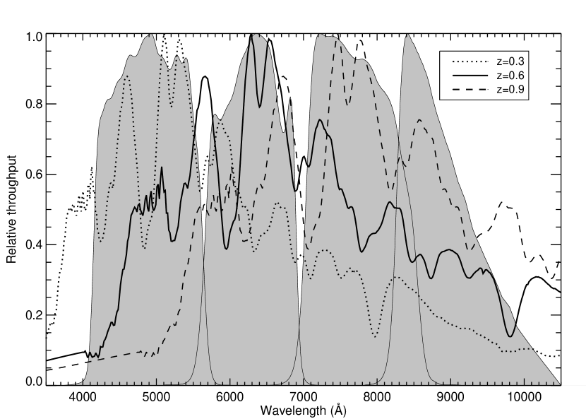
Figure 1: The mean effective responses of the $g^{\prime}$, $r^{\prime}$, $i^{\prime}$, and $z^{\prime}$ filters used in CFHT-LS, shown shaded left to right in the figure. The filter responses are those measured by CFHT, additionally multiplied by the reflectivity of the primary mirror, the throughput of the wide-field corrector optics, and the typical Megacam CCD quantum efficiency. Plotted underneath is a maximum-light $s=1$ SN Ia spectrum at redshifts of 0.3 (dotted), 0.6 (solid) and 0.9 (dashed), spanning the range of SNe Ia followed by the SNLS. The SN template is a revised version from Nugent et al. (2002).

The SN spectrum is then scaled to the expected effective $B$-band magnitude for that phase (assuming an $\Omega_{M}=0.30$, $\Omega_{\Lambda}=0.70$ cosmology), the stretch-luminosity relationship and the dispersion in peak magnitude from $\mathrm{d}m$ are applied, host extinction is applied, the spectrum is redshifted, and finally Milky Way extinction is applied. The spectrum is then integrated through the SNLS filters to generate an apparent magnitude in each filter, and the Megacam zeropoints used to calculate the counts in that filter given the exposure times listed in Table 2. The Megacam filter responses are those measured and provided by CFHT, and are additionally multiplied by the reflectivity of the CFHT primary mirror, the throughput of the wide-field corrector plus optics, and the average Megacam CCD quantum efficiency. These effective filter responses can be seen in Figure 1, together with a typical SN Ia spectrum at a range of redshifts typical of SNLS candidates.

Poisson noise, a filter-dependent sky noise (measured from real data in dark and gray sky conditions), and a filter-dependent systematic “flat-field error” noise is added to the predicted counts, and the counts converted back into fluxes using the original zeropoint, but with an additional zeropoint uncertainty ($\sigma=0.05$ mag) applied, typical of that present in real-time SNLS data (the zeropoint uncertainty for the final photometry is 0.02 mag or less, see Astier et al., 2005). Additional systematic noise is added to the $z^{\prime}$ (and a smaller amount in $i^{\prime}$) data to account for the imperfect fringe correction in real-time data. The result is a set of observations which should closely match real SNLS data. These synthetic SN observations are then passed to the SN selection code, and the code is run to locate the best-fitting SN parameters. This experiment was repeated for 2000 synthetic SNe. The final population of SNe has the following percentage composition: SNe Ia 50%, SN Ib/c 25%, SN IIL 8%, SN IIP 8%, and SN IIn 8%.

3.3 Simulation Results for SNe Ia

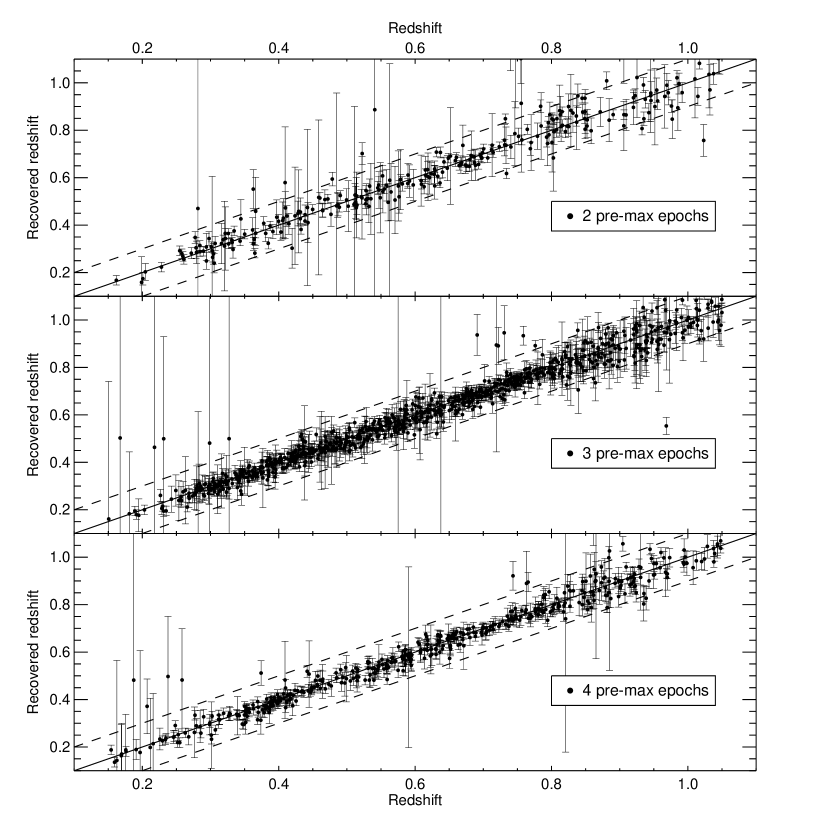
Figure 2: Results of the SN selection code run on a synthetic dataset of 2000 SNe Ia generated with observational parameters similar to that found in the SNLS (see $\S$ 3.2 for simulation details). This figure shows the comparison of actual and recovered redshift, and how this varies depending on the number of pre-maximum light-curve epochs are used in the fit, excluding pre-SN explosion epochs, from 2 epochs (top panel) to 4 epochs (lower panel). Only pre-maximum light data (including epochs of non detections) are used when recovering the redshift. On each epoch, 3 filters are observed, either $g^{\prime}r^{\prime}i^{\prime}$ or $r^{\prime}i^{\prime}z^{\prime}$.

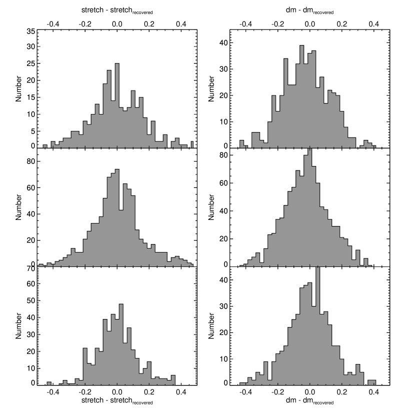
Figure 3: As Figure 2, but showing the distribution of actual minus recovered stretch (left panels), and for $\mathrm{d}m$ (right panels).

We now examine the results of the fits to the simulated SN Ia photometry (the core collapse SNe are discussed in Section 5). In Figures 2 and 3 we compare the results of the input and recovered SN Ia parameters. This figure shows the comparison of actual versus recovered redshift, and the difference in the recovered stretch and $\mathrm{d}m$ parameters. We also show how the accuracy of the recovered parameters depends on the number of data epochs in the SN light-curve which are available at the time of fitting (i.e. 2, 3 or 4 pre-maximum light epochs). The mean and standard deviations of these distributions are shown in Table 3. Fits made to the entire light-curve were also run (i.e. including post-maximum light data); the results were very similar to Figure 2, with the exception that the distributions in stretch and $\mathrm{d}m$ are significantly tighter (see Table 3), as would be expected when there is more information available to constrain these parameters.

For these synthetic, normal SNe Ia, the SN selection code appears capable of recovering their parameters without any apparent bias, even when only considering pre-maximum light data and when unknown zeropoint uncertainties and dispersions in the SN properties are included. Furthermore, the estimates of redshift are good to $\lesssim 0.1$ even when only two pre-maximum light-curve epochs are used in the fits.

However, these SN Ia simulations do not address three important questions. First, do our synthetic SNe Ia successfully represent normal observed SNe Ia? Is the code capable of recovering all types of SNe Ia without any bias against certain parts of SN Ia parameter space? Though our simulations generate SNe Ia that should encompass the full observed range of low-redshift SN Ia properties, the possibility that some characteristics of SNe Ia are not represented, or that the code may reject them as SNe Ia, cannot be ignored. Secondly, is our selection technique capable of distinguishing non-SN Ia events (e.g., core-collapse SNe) from true SN Ia events on early-time data (of great importance in a rolling-search)? Thirdly, does the choice of the cosmology used in the light-curve fit (equation (3)) bias the SNe Ia that are selected for spectroscopic follow-up? We address these questions in the next two sections, using both the simulations described above, and using empirical data on spectroscopically confirmed SN events discovered via the SNLS. In Section 4, we describe the relevant aspects of the SNLS, and discuss the application of the SN selection code to the SNLS in Section 5.

4 Application to the SNLS

In this section, we describe the application of the SN selection code to real-time data obtained as part of the SNLS. The results of the analysis, and a comparison with the simulations of Section 3, are then described in Section 5.

4.1 SNLS Real-time data reduction

A real-time reduction of the data are automatically performed by the CFHT-developed Elixir data reduction system (Magnier & Cuillandre, 2004), which performs basic de-trending of the images, including bias-subtraction, flat-fielding and a basic fringe subtraction in the $i^{\prime}$ and $z^{\prime}$ filters. This real-time analysis is somewhat different to that of the final Elixir reductions released through the Canadian Astronomy Data Centre (CADC). Final processed data are able to use all data taken during a given queue run to construct master flat-fields and fringe frames, which is not possible in real-time where library versions of these calibration frames from the previous queue run are used. In particular, flat-fielding and, in the case of $z^{\prime}$ data, fringe subtraction are both inferior in real-time data.

The Elixir-reduced data are then processed through two independent search pipelines, written by members of the SNLS collaboration in Canada and France, from which combined candidate lists are generated. The two pipelines typically produce candidate lists which agree at the 90% level down to $i^{\prime}\simeq 24.0$. In this paper, we refer exclusively to the Canadian pipeline, though the details of the French pipeline are similar in most respects. Full details of these reductions will be presented in forth-coming papers; here we present a brief overview. We perform a photometric alignment to secondary standards within each field using a multiplicative scaling factor, and astrometrically align the data in different filters using custom-built astrometric reference catalogs. Finally, the frames are re-sampled to a common pixel coordinate system, and a median stack in each filter is generated, rejecting cosmic-ray events and other chip defects.

The point-spread functions (PSFs) of the image stack and the deep reference image constructed from observations from the previous year are matched using a variable kernel technique, and a subtraction image generated containing only sources which have varied since the reference epoch. This subtraction image is searched for SN candidates using automated techniques, with all likely candidates screened by a human eye to ensure obviously non-stellar sources are not included on the potential candidate follow-up list.

PSF-fit and aperture photometry for all new and previously detected sources is measured and the flux information is stored in a publicly-available database of all SN candidates. New candidates are automatically cross-correlated with the database of existing variable sources (to identify previously known AGN and variable stars), and back-tracked through previous epochs in order to construct as much information as possible as to their nature. Additionally, each candidate is given a provisional category of either likely supernovae (SN), likely AGN (if the detection is precisely centered and appears intermittently over long periods of time), likely variable star (if the candidate host appears stellar and PSF-like), or likely moving object (if the candidate moves between epochs). Where any reasonable doubt exists, the SN classification is retained. The result is a database of flux information for every variable candidate detected in the SNLS.

Spectroscopic follow-up for the SNLS is currently provided by dedicated follow-up programs on the European Southern Observatory Very Large Telescope (VLT; 60 hours/period), Gemini North and South (60 hours/semester) and Keck-I/II telescopes (4 nights in the “A” semester of each year), as well as other programs at Keck-I making detailed studies of select SNe (4-8 nights a year). During the time-frame covered by this paper, the VLT observed 61 candidates (Basa et al., 2005 in prep.), Gemini observed 40 candidates (Howell et al., 2005) and Keck observed 21 candidates, 7 as part of routine follow-up, and 14 for a detailed study program (Ellis et al., in prep.) Some candidates were observed on more than one occasion. Full details of the reductions and SN typing methods employed can be found in the papers referenced above. Typically, redshifts are determined from host galaxy spectral emission or absorption features, or via a $\chi^{2}$ template matching technique to a large library of local SN spectra of all types (Howell et al., 2005).

4.2 Analysis

The photometry and candidates that we use in this analysis are taken from the Canadian real-time analysis corresponding to the period May 2004 to January 2005 – or approximately 3 “field-seasons”. Over this period, the SN selection code was used to assist in the selection of spectroscopic follow-up candidates. 440 potential SN candidates were located by our real-time analysis software (excluding likely AGN and variable stars), of which 121 were followed spectroscopically. Of these, 70 have since been identified as SNe Ia or probable SNe Ia (denoted SN Ia* hereafter), 6 as being consistent with an SN I, 11 as SNe II, 4 as SN Ib/c. 30 candidates remain unidentified or are non-SN events. During this period, in order to test the SN selection code, in some months we deliberately followed events that were predicted not to be SNe Ia to ensure we were not biasing against particular classes of SN Ia events.

For this analysis, we run the SN selection code on all SN candidates discovered during this period (fixing $E_{B-V}^{\small\mathrm{mw}}$ as appropriate for each candidate), firstly fitting on the entire real-time light-curve, and secondly fitting just the data that were available at the time the follow-up decision was made. This exact date was not accurately recorded or easily reconstructed for all events; we approximate this by cutting-off the real-time light-curves at 2 days before maximum light in the SN rest-frame. Clearly, this cut restricts us to only consider candidates with at least 2 epochs prior to 2 days before maximum light, $\sim 95$% of the total SN Ia sample; furthermore, the approximation may lead to some fits using more data (and some less) than was actually used at the time the follow-up decision was made.

5 Results

5.1 Discriminating core-collapse SNe from SNe Ia

We first examine the non-SN Ia events located by the SNLS. One important requirement of the SN selection technique is to not only return the most likely parameters describing a SN based on the fitting the real-time light-curve to a normal SN Ia model, but also to return some guide as to the likelihood that the target is indeed a normal SN Ia. As fits to non-SNe Ia should be of lower quality, we examine the $\chi^{2}$ of the light-curve fits to examine whether it can be used as a reliable indicator.

The most common form of contamination in our sample comes from core-collapse SNe. While AGN and variable stars are obviously present, they are usually easily screened out as they show significant variation on the time-scale of a year, and are usually already present in our database of variable objects. Core collapse SNe – the various sub-classes of SNe II and SNe Ib/c – are heterogeneous; the range in peak magnitudes (Richardson et al., 2002), spectra (Matheson et al., 2001), and colors can be considerable. The general trend however is that for a core-collapse SN and a SN Ia located at the same redshift, the core collapse SN will be fainter than the SN Ia. Typical SNe II are 1-2.5 mag fainter at peak than SNe Ia, and typical SNe Ib/c around 1.5 mag fainter (see table 1 in Richardson et al., 2002), though there are examples of more luminous or peculiar events in the literature (e.g. Germany et al., 2000; Turatto et al., 2000).

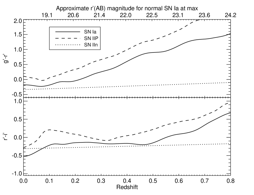
Figure 4: The observed $g^{\prime}-r^{\prime}$ and $r^{\prime}-i^{\prime}$ colors of SNe Ia compared to some SNe II models as a function of redshift. As SNe Ia typically appear 1-2 mag brighter than SNe II located at the same redshift, the strong evolution in SN Ia $g^{\prime}-r^{\prime}$ color with redshift provides a strong discriminant against core-collapse SNe, which appear too blue for a redshift based on a SN Ia fit.

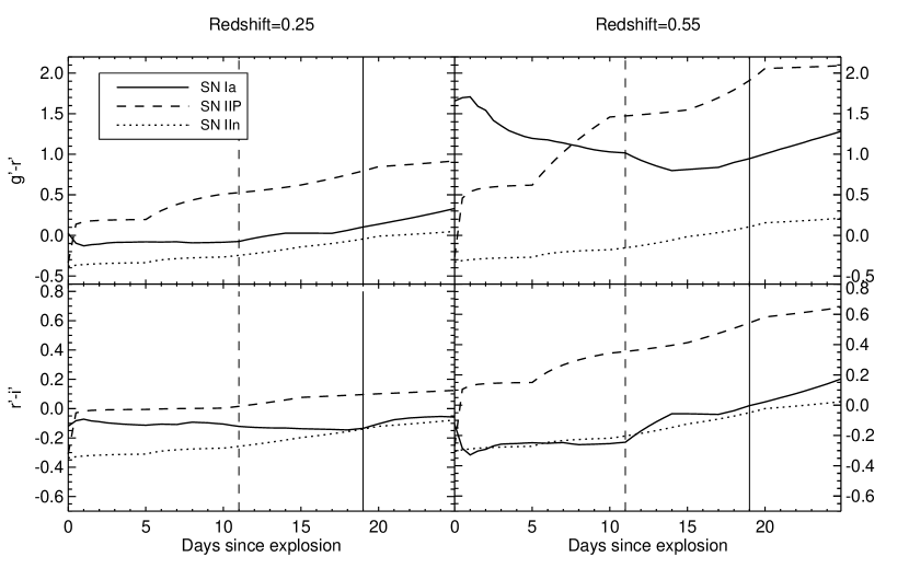
Figure 5: The observed $g^{\prime}-r^{\prime}$ and $r^{\prime}-i^{\prime}$ colors of SNe Ia compared to some SNe II models as a function of rest-frame phase of the SN. Two redshifts are shown; $z=0.25$ and $z=0.55$. Note that SNe II and SNe Ia peak at different times after explosion; these are indicated with different vertical lines in the figure.

Our SN Ia selection technique uses both this peak magnitude information and the color of the observed light-curve, fitting a given candidate for redshift, phase, stretch, extinction, and dispersion in the peak magnitude under the assumption that the object is a SN Ia in an assumed cosmology. This places a constraint on the redshift that can be fit (as SNe Ia are calibrated candles and have similar intrinsic luminosities), and hence restricts the range of observed colors that are consistent with a SN Ia as a function of SN brightness. We demonstrate this in Fig. 4, where we show the redshift evolution in the color of a SN Ia and two example models for a SN II (in this case an SN IIP and an SN IIn), and Fig. 5, where we show the evolution of SN colors as a function of phase. The SN Ia template is that discussed in Section 2.2 and the core-collapse templates are described in Section 3.2.

Consider a SN IIP at maximum light located at $z=0.25$ with $g^{\prime}-r^{\prime}\sim 0$ and $r^{\prime}\sim 23$. Though the color is also consistent with a maximum-light SN Ia at the same redshift (Fig. 4), the peak magnitude of the SN IIP is around 2 magnitudes fainter than a SN Ia would be ($r^{\prime}\sim 21$). This $r^{\prime}\sim 23$ peak magnitude is consistent with a SN Ia at $z\simeq 0.55$; however, at this redshift the $g^{\prime}-r^{\prime}$ color of a normal SN Ia is $\sim$1 mag redder. Hence, SNe II (and other core-collapse events) can potentially be screened out by searching for objects that appear too blue in $g^{\prime}-r^{\prime}$ for the fitted redshift when compared to the SN Ia model, or more precisely, rejecting objects that have a large $\chi^{2}$ per degree of freedom (d.o.f) in the $g^{\prime}$-band from the SN Ia fit. A measurement of color at exactly maximum light is not required; the same trend is apparent up to about 20 days after explosion (Fig. 5).

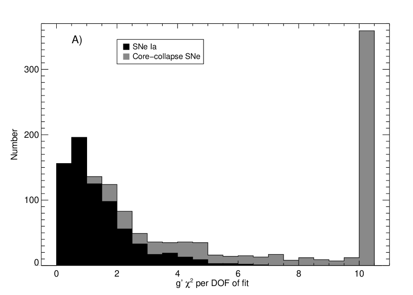
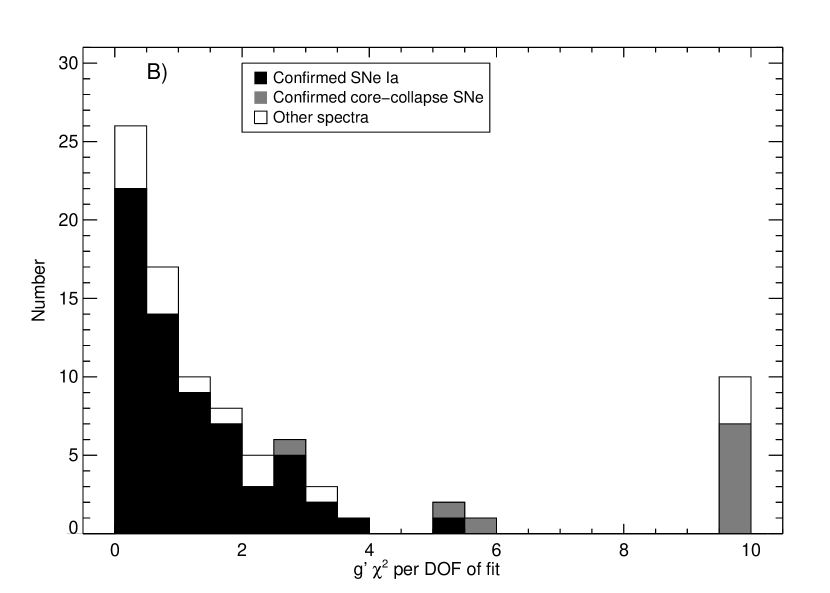
Figure 6: The distribution of $g^{\prime}$ $\chi^{2}$ per d.o.f. for the fits of all SN candidates for the simulations (Panel a, left; Section 3) and for real SNe discovered by SNLS (Panel b, right). In panel a) ‘Core collapse SNe’ represent all the various sub-types of core-collapse SNe as described in the text. In panel b), ‘Confirmed SNe Ia’ are those SNe identified as either ‘Ia’ or ‘Ia*’ from their spectra, ‘Confirmed core collapse SNe’ are those identified as any variant of a SN II, ‘Other spectra’ includes any other object observed spectroscopically regardless of the type of object.

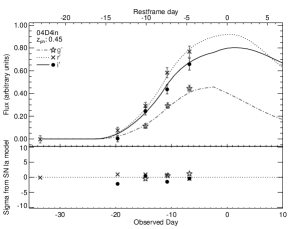
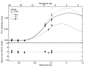
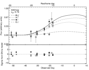
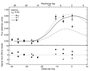
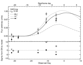
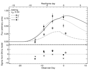
Figure 7: Example light-curve fits to early real-time photometry. In all cases the light-curves are fit to a SN Ia model, with the phase, redshift and stretch free parameters in the fit as described in the text. The top row shows fits to known SNe Ia; from left to right 04D4in ($z=0.52$), 04D4jr ($z=0.48$), and 04D1ow ($z=0.92$). The bottom row shows fits to known core-collapse SNe; from left to right: 04D1ln (SN IIP; $z=0.21$), 04D1me (SN IIP; $z=0.30$), and 04D1la (SN Ib/c; $z=0.32$). In all cases, the deviations from the SN Ia model are significantly larger for the core-collapse SNe, allowing an efficient identification of such objects based on the $g^{\prime}$ $\chi^{2}$.

The distributions of $\chi^{2}$ in the $g^{\prime}$-band from our pre-maximum light fits to the simulated and real SNLS candidates are shown in Fig. 6. Example light-curve fits to both real SNe Ia and real core collapse SNe are shown in Fig. 7. As expected, the SNe Ia and core collapse SNe have quite different distributions, both for the simulated survey data, and for the real survey data. SNe Ia typically have a small $\chi^{2}$; the median value is 0.85 (1.01 for the simulated data), and 90% of SNe Ia have $\chi^{2}<2.80$ ($\chi^{2}<2.91$ in the simulations). Only 1% (0.9% in simulated data) have $\chi^{2}>5$.

The $\chi^{2}$ for core collapse SNe is typically larger, with 10 of 11 events having a $\chi^{2}>5$; all SNe II have $\chi^{2}>5$. The numbers for the fits to the simulated SNe are similar; 80% of simulated core-collapse SNe have a $\chi^{2}>5$. Thus, the $\chi^{2}$ in the observed $g^{\prime}$ filter seems an efficient discriminant with which to remove the majority of core collapse SNe from spectroscopic follow-up samples.

5.2 Redshift and phase precision

The accuracy to which redshift and phase can be estimated are important quantities; the first allows an optimal spectrograph setting to be used, and the second ensures that SNe are observed at a phase when the different sub-types show the most diversity and with the greatest contrast over their host galaxy. Here we investigate how well the predicted redshift and phase of the SNe Ia agree with actual values.

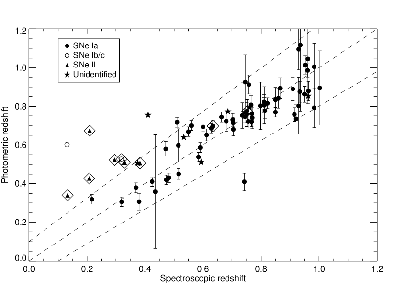
Figure 8: The comparison between $z_{\mathrm{phot}}$ and $z_{\mathrm{spec}}$ for the candidates followed as part of the SNLS. The photometric redshifts are from the SN and are based on pre-maximum-light data only. The SN are coded according to the type of the event, and those events that would have been removed from our follow-up sample based purely on the $g^{\prime}$ $\chi^{2}$ (per d.o.f.) from the SN Ia fit are boxed with a diamond. The two rejected SNe Ia have only poor quality pre-maximum light data; in reality more data was utilized for these candidates before a follow-up decision was made. The $z_{\mathrm{phot}}$ errors are those reported by the least-squares minimizer. The over-plotted dashed lines show a 1:1 correspondence between $z_{\mathrm{phot}}$ and $z_{\mathrm{spec}}$ as well as $\pm$10% in $(1+z)$. The assumed cosmology is $\Omega_{M}=0.25$, $\Omega_{\Lambda}=0.75$, and the SNe Ia include both ‘Ia’ or ‘Ia*’ events.

The photometric-redshift ($z_{\mathrm{phot}}$) versus spectroscopic-redshift ($z_{\mathrm{spec}}$) comparison for all spectroscopically observed objects where a $z_{\mathrm{spec}}$ could be determined is shown in Fig. 8. The plot is based on fits to just the data that was available at the time the follow-up decision was made (taken as pre-maximum light data).

The agreement between $z_{\mathrm{phot}}$ and $z_{\mathrm{spec}}$ for SNe Ia is remarkably good. The median $\left|\Delta z\right|/(1+z_{\mathrm{spec}})$ is 0.031, with 90% of the SNe Ia having $\left|\Delta z\right|/(1+z_{\mathrm{spec}})<0.08$. The agreement for other SN types is, as expected, much poorer, as the differing colors, light-curves shapes and brightnesses of these SN leads to an incorrect redshift estimate. However, most of these core collapse candidates are rejected by the code as being SNe Ia due to the $\chi^{2}$ of the fits; such rejected SNe are marked on the figure. As a comparison, Fig. 9 shows the $z_{\mathrm{phot}}$ versus $z_{\mathrm{spec}}$ for fits based on the entire SN light-curve; here the median $\left|\Delta z\right|/(1+z_{\mathrm{spec}})$ is 0.025. Note that the apparent high accuracy of this technique does not mean that spectroscopic redshifts are not needed for cosmological analysis; clearly as a cosmology is assumed in order to derive the fitted redshift, this redshift could not then be used to re-derive cosmological constraints. Furthermore, as the nature of the events are not known to be SNe Ia a priori, and the assumed cosmology is a very useful prior when identifying the core collapse SNe, the technique could not be used to derive cosmological constraints (as can be done in some low-redshift SN Ia samples, e.g. Barris & Tonry, 2004) without a significant improvement in our knowledge of the color evolution and light-curve morphology of core collapse SNe.

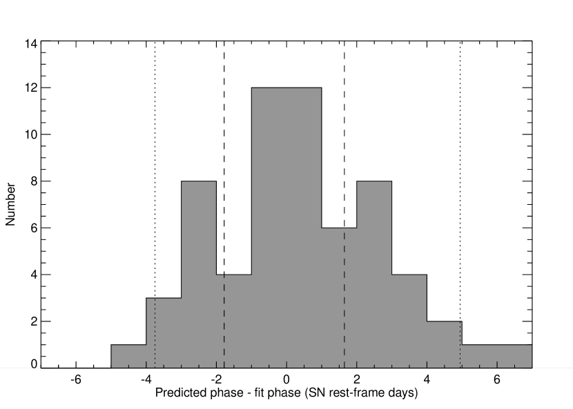
Figure 10: The distribution of the predicted time of maximum light minus the actual time of maximum light in the SN rest-frame. The “predicted time of maximum light” is based only on pre-maximum light light-curve data i.e. the data available at the time of spectroscopic follow-up. The “actual time of maximum light” is based on the entire SN light-curve. The vertical lines denote the region containing 50% (dashed) and 90% (dotted) of all candidates. Only confirmed SNe Ia (or SNe Ia*) with spectroscopic redshifts are shown. The uncertainty on the time of maximum light from fits based on the entire light-curve is $\sim 0.5-1.0$ days.

The distribution of the predicted date of maximum light versus the date of maximum light based on the entire light-curve is shown in Fig. 10 (as before, predicted values are only based on candidate light-curves up to 2 rest-frame days before maximum light). The agreement is good, with 50% of the predicted times of maximum light lying within $\pm 1.75$ rest-frame days of the actual date of maximum light, and 90% within $\pm\sim 4$ days.

5.3 Effect of assumed cosmology

In this section, we investigate any possible bias in the population of objects that would be selected for spectroscopic follow-up based on the “assumed” cosmology that is used in the light-curve fit. We repeat the SN selection fits on the real survey data using a different cosmological model, and compare the identity of the rejected candidates with those rejected when using the standard cosmology.

Subtle changes in the cosmology, for example varying the value of the equation of state parameter $w$, have no effect on the nature of the candidates that are rejected. For example, the candidates that are rejected (or selected) with $w=-1$ are also rejected (or selected) with $w=0.8$ or $w=-1.2$, as the differences in the apparent-magnitude/redshift relation are very small. A more drastic test is to compare to a cosmology that makes very different predictions in the apparent magnitude of an object as a function of redshift. We compare to an Einstein-de-Sitter (EdS) cosmology ($\Omega_{M}=1.0$, $\Omega_{\Lambda}=0.0$); the apparent magnitude of a SN Ia differs by $\simeq 0.5$ mag at $z=0.6$. Any bias in the objects that are selected for follow-up by assuming an accelerating universe cosmology should be evident after these fits.

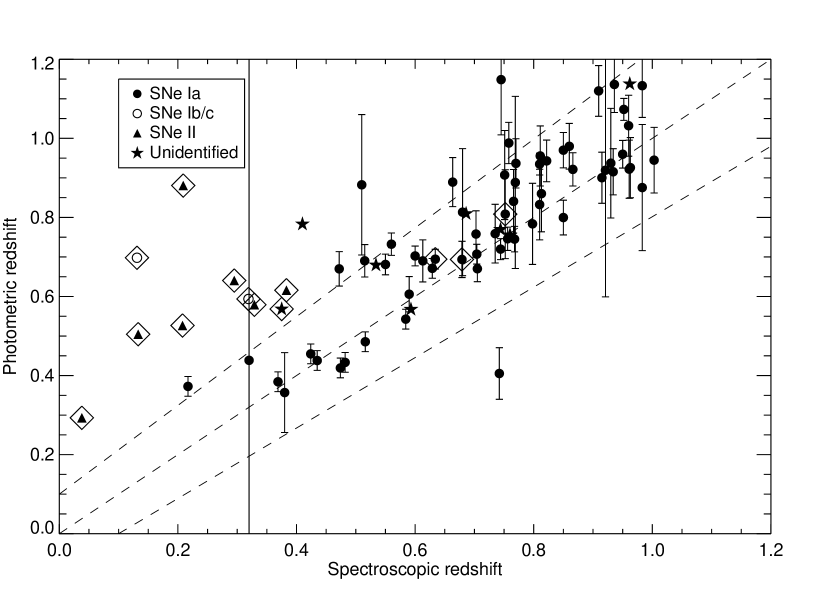
Figure 11: As Fig. 8, but assuming an $\Omega_{M}=1.0$, $\Omega_{\Lambda}=0.0$ cosmology. Changing the assumed cosmology does not alter the SNe that are rejected as being SNe Ia by the fitting code, though the agreement between $z_{\mathrm{spec}}$ and $z_{\mathrm{phot}}$ is poorer.

In Fig. 11 we show the same $z_{\mathrm{phot}}$ versus $z_{\mathrm{spec}}$ comparison as in Fig. 8, but for the EdS Universe. There is a clear offset apparent in these plots; in an EdS Universe, the $z_{\mathrm{phot}}$ is found to be systematically larger than the $z_{\mathrm{spec}}$, and the size of this effect increases at higher redshift. This is simple to understand; in a EdS universe, objects appear brighter than in a $\Lambda$-cosmology at the same redshift. If we live in a $\Lambda$-dominated Universe, the SN selection code will over-estimate the redshift (i.e. will try to make the objects fainter) if it assumes an EdS cosmology.

The objects that are rejected based on the $g^{\prime}$ $\chi^{2}$ are the same when assuming an EdS Universe as when assuming a $\Lambda$-cosmology i.e. the assumed cosmology does not place a strong constraint on the objects that are selected for spectroscopic follow-up. However, assuming a $\Lambda$-cosmology does improve our estimates of candidate redshifts and hence stretches and observer-frame ages, which is essential to ensure that candidates are observed at the optimal time (Howell et al., 2005). The assumed cosmology does not provide the key discriminant in rejecting non-SN Ia events, but does enable a more efficient follow-up observation to be performed.

5.4 Implications for cosmological measurements

We now examine the SNe Ia that are rejected in any cosmology, i.e. SNe Ia that have sufficiently discrepant stretches, luminosities, or colors when compared to the standard template that is used in the fits, or SNe where the selection code simply fails to find the correct solution. If similar sub-types of SNe Ia were consistently rejected, this could introduce a bias in the types of SNe Ia that were sent for follow-up, with a possible consequent bias on the cosmological results that would be derived from the resulting spectroscopic sample. Alternatively, if the occasional rejections of a SN Ia were random, and related to the phasing of the observations or the poor quality of a given epoch of real-time data, then the impact on the derived cosmological parameters would be very small.

We investigate this effect using a simulated dataset similar to that in Section 3. We generate 700 high-redshift ($0.15<z<0.9$) SNe Ia (the SNLS end-of-survey goal), and combine with 300 local SNe Ia ($0.01<z<0.12$), a sample size equivalent to that likely to be available at the end of the SNLS from projects such as the Carnegie Supernova Project (Freedman, 2005) and the Nearby Supernova Factory (Aldering et al., 2002). The 700 high-redshift SNe are fit using the SN selection code, the pre-maximum light data fit, and those SNe which are formally rejected are noted. Typically 1-2% are formally rejected by the code, usually because of a lack of data before maximum light (due to weather in our simulations) rather than an intrinsic property of the SN. We then perform a full cosmological fit of $w$ and $\Omega_{M}$, firstly on the full 700+300 SN Ia sample, and then on the same sample less the few high-redshift SNe that were rejected by the SN selection code based on the pre-maximum light fits. The cosmological fits follow a similar method as that used in Astier et al. (2005), and produce confidence contours in $w$ and $\Omega_{M}$. In all cases, the input cosmological values were $\Omega_{M}=0.3$ and $w=-1$, and a flat Universe was assumed.

As each survey simulation generates different SNe, we repeat the full simulation four times; the confidence contours for the recovered cosmological parameters in $\Omega_{M}$ and $w$ are shown in Fig. 12. Constraints from the baryon acoustic oscillations (BAO) are also included (Eisenstein et al., 2005). The differences between the cosmological fits for the different samples are very small. In all cases, the difference in the derived value of $w$ is less than 0.001 ($\sim$0.02$\sigma$) when including the BAO constraints, and less than 0.015 ($\sim$0.05$\sigma$) when the BAO constraints are not used. We therefore conclude that the SN selection method adds no significant bias to the eventual cosmological results of the SNLS.

5.5 Potential SN Ia targets not followed spectroscopically

An alternative, more empirical, method of how successful the SN selection code is at locating candidates for follow-up in real-time, is to examine the fraction of good SN Ia candidates rejected by the code. The impact on the determination of the cosmological parameters of these SNe was shown to be negligible in the previous section; however, this is also important for future studies of the SN Ia that rely on near-complete spectroscopic samples of SNe Ia being available (e.g., SN rates). We assess this by examining the distribution of the fitted SN stretches of our candidates once their light-curves are complete. Virtually all normal SN Ia stretches lie in the range 0.7 to 1.3 (e.g. Perlmutter et al., 1999; Astier et al., 2005). SNe Ia with very different stretches have been discovered locally, for example the broad $s=1.6$ light-curves of very rare SN 2001ay-like SNe (Howell & Nugent, 2004) or the faint, fast declining SN 1991bg-like objects (e.g. Filippenko et al., 1992; Garnavich et al., 2004). Although SNe such as SN 1991bg have been shown to be calibrateable as standardized candles, and have been used in determinations of the Hubble constant (Garnavich et al., 2004), these classes of peculiar SNe are unlikely to be useful for cosmological studies at high-redshift – they may not follow the lightcurve-shape/luminosity relationship (in the case of SN 2001ay), and may be naturally selected against at high redshift due to their faintness (in the case of SN 1991bg-like SNe, which are around 2 magnitudes under-luminous). In “distance-limited” surveys, which likely provide a census of all types of SNe Ia, around 65% of SNe Ia appear spectroscopically “normal” (Li et al., 2001), a number which is probably a lower limit on the number of cosmologically useful SNe, as it excludes SN 1991T-like events that may still be calibrateable candles. This fraction will only rise in high-redshift searches as the fainter SN 1991bg-like SNe are selected against. Hence candidates with fitted stretches outside of the range 0.7 to 1.3 are either unlikely to be SNe Ia, or unlikely to be cosmologically useful SNe Ia, while those with $0.7<s<1.3$ are likely to be useful SNe Ia.

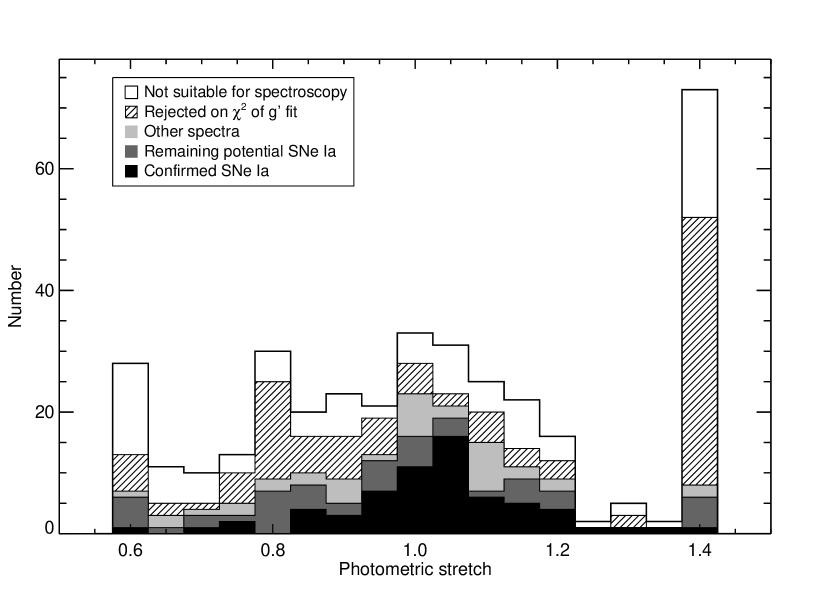
Figure 13: The histogram of fitted stretch for all SN candidates from the SNLS during the time period covered by this paper. ‘Confirmed SNe Ia’ are those SNe identified as either Ia or Ia* from their spectra, ‘Other spectra’ includes any other object observed spectroscopically regardless of the type of object that was not identified as a SN Ia, ‘Rejected on $\chi^{2}$ of $g^{\prime}$ fit’ includes all remaining objects that are rejected by the SN selection code based on the fit to the $g^{\prime}$-band light-curve, ‘Not suitable for spectroscopy’ includes all remaining objects which at maximum light are either too faint or have too low percentage increase for a likely successful spectroscopic observation, and ‘Remaining potential SNe’ includes all remaining objects which are not in the above categories and which are potentially SNe Ia not observed spectroscopically. The photometric parameters are based on photometric-redshift fits to the entire candidate light-curve. The peaks at $s=0.6$ and $s=1.4$ reflect the range over which stretch is allowed to vary in the fits ($0.6<s<1.4$).

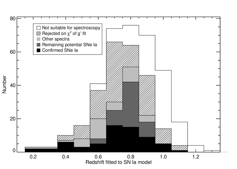
Figure 14: The histogram of SN Ia photometric redshifts for all candidates from the SNLS during the time period covered by this paper. The categories of objects are the same as in Fig. 13. The photometric redshift is based on fits to the entire candidate light-curve under the assumption that the object is a SN Ia; clearly for non-SNe Ia the $z_{\mathrm{phot}}$ will be inaccurate. The figure shows that there are few good candidates lying at $z_{\mathrm{phot}}<0.65$ which were rejected by the selection code in the real-time analysis. Note that the redshift distribution of the candidates ‘Rejected on $\chi^{2}$ of $g^{\prime}$ fit’ is not representative of the true redshift distribution of these events as these candidates are unlikely to be SNe Ia.

Figure 13 shows the distribution of fitted stretch for all candidates (even if the spectroscopic redshift is known, redshift is not fixed in these fits). As expected, the stretches for the spectroscopically confirmed SNe Ia lie in the expected range 0.7 to 1.3. Furthermore, of the candidates not selected by the code for spectroscopic follow-up, few appear to be good candidates for normal SNe Ia once objects for which a spectroscopic observation would be too challenging have been removed. Objects which were not possible to observe spectroscopically are defined as those for which the peak $i^{\prime}$ magnitude is $>24.25$, or for which the peak $i^{\prime}$ percentage increase over the host galaxy is $<30$%. (SNe that do not meet these cuts are rarely positively identified – see Howell et al. 2005) Fig. 14 shows the same objects broken-down into the same categories, but the histogram is of the fitted redshift rather than the stretch. As would be expected, objects defined as too difficult to attempt spectroscopically are only found at $z>0.65$, where the contrast over the host galaxy is typically smaller as the hosts have a smaller apparent size on the sky - the angular separation between SN and host is smaller, and the SN light becomes more mixed with the galaxy light. At $z<0.65$, of all the total SN candidates that were consistent with a SN Ia, only $\sim 5$% were not followed spectroscopically where an observation would have been possible.

6 Summary

In this paper, we have presented a selection technique for high-redshift supernovae searches that can be used to identify SNe Ia after only 2-3 epochs of multi-band photometry. Using both simulated SN data and the SNLS real-time data as a test-case, we have shown that the technique is able to discriminate between SNe Ia and core collapse SNe (SNe II, SNe Ib/c) based on the quality of the fit in the $g^{\prime}$ filter. For SNe Ia, the technique accurately predicts the redshift, phase and light-curve parameterization of these events to a precision of $\left|\Delta z\right|/(1+z_{\mathrm{spec}})<0.09$ in redshift, and $\pm$2-3 rest-frame days in phase, and there is no apparent bias on cosmological parameters derived using SNe Ia selected in using this method.

The technique is now routinely used within the SNLS to help select priority candidates for spectroscopic follow-up and confirmation as SN Ia for use as standard candles in the derivation of cosmological parameters (Astier et al., 2005); the improvement in spectroscopic success the method brings is discussed elsewhere (Howell et al., 2005). These techniques will be used in other current and future planned surveys, which are likely to be “spectroscopically starved”, with many more candidates than can be followed up.

The obvious extension to this method will be when “final” data (versus the real-time data used here) becomes available for SNLS. With many of the real-time uncertainties removed, and a high quality fringe subtraction capable of removing systematics, this SN selection technique will provide a logical method for determining the types and redshifts for the many hundreds of SNe that it is not possible to observe spectroscopically, particularly when combined with photometric redshifts for the host galaxies that will be routinely available for the CFHT-LS Deep Fields. Such a combination of data would allow a calculation of the rates of all SN types out to $z=1$.

Table 1: CFHT-LS Deep field locations

Field	RA (J2000)	DEC (J2000)	Other data
D1	02:26:00.00	$-$04:30:00.0	XMM-Deep, VIMOS, SWIRE, GALEX, VLA
D2	10:00:28.60	+02:12:21.0	COSMOS/ACS, VIMOS, SIRTF, GALEX, VLA
D3	14:19:28.01	+52:40:41.0	(Groth strip); DEEP-2, SIRTF, GALEX
D4	22:15:31.67	$-$17:44:05.7	XMM-Deep, GALEX

Table 2: Exposure times and epochs for a typical month in SNLS

	Epoch 1	Epoch 2	Epoch 3	Epoch 4	Epoch 5
$\sim$Days w.r.t. new moon:	-8	-4	0	+4	+8
$g^{\prime}$	5$\times$225s	$\cdots$	5$\times$225s	5$\times$225s	$\cdots$
$r^{\prime}$	5$\times$300s	5$\times$300s	5$\times$300s	5$\times$300s	5$\times$300s
$i^{\prime}$	7$\times$520s	5$\times$360s	7$\times$520s	5$\times$360s	7$\times$520s
$z^{\prime}$	10$\times$360s	$\cdots$	10$\times$360s	$\cdots$	10$\times$360s

Table 3: “actual minus recovered” SN parameters for the 2000 synthetic SNe Ia

Parameter	Simple		Outlier resistant
	Mean	$\sigma$	Mean	$\sigma$
Pre-maximum light-curve epochs only:
$z-z_{\mathrm{recovered}}$	0.098	0.240	0.007	0.025
$s-s_{\mathrm{recovered}}$	0.204	0.423	0.015	0.131
$\mathrm{d}m-\mathrm{d}m_{\mathrm{recovered}}$	-0.004	0.144	-0.004	0.140
Entire light-curve:
$z-z_{\mathrm{recovered}}$	0.006	0.041	0.007	0.022
$s-s_{\mathrm{recovered}}$	0.041	0.099	0.021	0.044
$\mathrm{d}m-\mathrm{d}m_{\mathrm{recovered}}$	0.010	0.142	0.012	0.132

Figure 9: As Fig. 8, but using the entire light-curve in the fit rather than just the pre-maximum light data. Note that more SNe appear on this plot than on Fig. 8, as this plot includes SNe for which there is no pre-maximum light data.

Figure 12: The cosmological fits in $w$ and $\Omega_{M}$ to four simulated SNLS-like SN samples with and without the few SNe Ia formally rejected by the SN selection code. Each panel represents a different SNLS-like survey; the differing positions of the contours is expected and arises from random variation from simulation to simulation. In each panel, the solid contours indicate the full sample of 700 SNLS SNe plus 300 low-redshift SNe, the dotted lines are the same sample minus those high-redshift SNe rejected by the SN selection code. In each case, the confidence contours with and without the baryon acoustic oscillations constraint (dashed line; Eisenstein et al., 2005) are shown. The number in each panel indicates the number of high-redshift SNe not rejected by the selection code.

References

- Aldering et al. (2002) Aldering, G., et al. 2002, in Survey and Other Telescope Technologies and Discoveries. Edited by Tyson, J. Anthony; Wolff, Sidney. Proceedings of the SPIE, Volume 4836, pp. 61-72 (2002)., 61–72
- Astier et al. (2005) Astier, P., et al. 2005, A&A, in press, astroph/0510447
- Barris & Tonry (2004) Barris, B. J. & Tonry, J. L. 2004, ApJ, 613, L21
- Barris et al. (2004) Barris, B. J., et al. 2004, ApJ, 602, 571
- Bessell (1990) Bessell, M. S. 1990, PASP, 102, 1181
- Bohlin & Gilliland (2004) Bohlin, R. C. & Gilliland, R. L. 2004, AJ, 127, 3508
- Cardelli et al. (1989) Cardelli, J. A., Clayton, G. C., & Mathis, J. S. 1989, ApJ, 345, 245
- Dahlén & Goobar (2002) Dahlén, T. & Goobar, A. 2002, PASP, 114, 284
- Di Carlo et al. (2002) Di Carlo, E., et al. 2002, ApJ, 573, 144
- Eisenstein et al. (2005) Eisenstein, D. J., et al. 2005, ArXiv Astrophysics e-prints
- Filippenko et al. (1992) Filippenko, A. V., et al. 1992, AJ, 104, 1543
- Freedman (2005) Freedman, W. L. . T. C. S. P. 2005, in ASP Conf. Ser. 339: Observing Dark Energy, 50–+
- Gal-Yam et al. (2004) Gal-Yam, A., Poznanski, D., Maoz, D., Filippenko, A. V., & Foley, R. J. 2004, PASP, 116, 597
- Garnavich et al. (2004) Garnavich, P. M., et al. 2004, ApJ, 613, 1120
- Garnavich et al. (1998) Garnavich, P. M., et al. 1998, ApJ, 493, L53+
- Germany et al. (2000) Germany, L. M., Reiss, D. J., Sadler, E. M., Schmidt, B. P., & Stubbs, C. W. 2000, ApJ, 533, 320
- Gilliland et al. (1999) Gilliland, R. L., Nugent, P. E., & Phillips, M. M. 1999, ApJ, 521, 30
- Goldhaber et al. (2001) Goldhaber, G., et al. 2001, ApJ, 558, 359
- Goobar & Perlmutter (1995) Goobar, A. & Perlmutter, S. 1995, ApJ, 450, 14
- Guy et al. (2005) Guy, J., Astier, P., Nobili, S., Regnault, N., & Pain, R. 2005, in A&A, in press, astroph/0506583
- Höflich et al. (2000) Höflich, P., Nomoto, K., Umeda, H., & Wheeler, J. C. 2000, ApJ, 528, 590
- Höflich et al. (1998) Höflich, P., Wheeler, J. C., & Thielemann, F. K. 1998, ApJ, 495, 617
- Hamuy et al. (1995) Hamuy, M., Phillips, M. M., Maza, J., Suntzeff, N. B., Schommer, R. A., & Aviles, R. 1995, AJ, 109, 1
- Hamuy et al. (1996) Hamuy, M., Phillips, M. M., Suntzeff, N. B., Schommer, R. A., Maza, J., & Aviles, R. 1996, AJ, 112, 2391
- Howell & Nugent (2004) Howell, D. A. & Nugent, P. 2004, in Cosmic Explosions in Three Dimensions, ed. P. Höflich, P. Kumar, & J. C. Wheeler, 151
- Howell et al. (2005) Howell, D. A., et al. 2005, ApJ, in press, astro-ph/0509195
- Jha (2002) Jha, S. 2002, Ph.D. Thesis
- Jha et al. (2005) Jha, S., Kirshner, R. P., Challis, P., Garnavich, P. M., & Matheson, T. 2005, AJ, in press, astro-ph/0509234
- Jorge et al. (1980) Jorge, J. M., Burton, S. G., & H., K. E. 1980, User Guide for MINPACK-1, Tech. Rep. ANL-80-74, Argonne National Laboratory, Argonne, IL, USA
- Knop et al. (2003) Knop, R. A., et al. 2003, ApJ, 598, 102
- Krisciunas et al. (2005) Krisciunas, K., et al. 2005, AJ, in press, astro-ph/0508681
- Lentz et al. (2000) Lentz, E. J., Baron, E., Branch, D., Hauschildt, P. H., & Nugent, P. E. 2000, ApJ, 530, 966
- Levan et al. (2005) Levan, A., et al. 2005, ApJ, 624, 880
- Li et al. (2001) Li, W., Filippenko, A. V., Treffers, R. R., Riess, A. G., Hu, J., & Qiu, Y. 2001, ApJ, 546, 734
- Magnier & Cuillandre (2004) Magnier, E. A. & Cuillandre, J.-C. 2004, PASP, 116, 449
- Matheson et al. (2001) Matheson, T., Filippenko, A. V., Li, W., Leonard, D. C., & Shields, J. C. 2001, AJ, 121, 1648
- Nobili et al. (2003) Nobili, S., Goobar, A., Knop, R., & Nugent, P. 2003, A&A, 404, 901
- Nugent et al. (2002) Nugent, P., Kim, A., & Perlmutter, S. 2002, PASP, 114, 803
- O’Donnell (1994) O’Donnell, J. E. 1994, ApJ, 422, 158
- Oke & Gunn (1983) Oke, J. B. & Gunn, J. E. 1983, ApJ, 266, 713
- Peebles & Ratra (2003) Peebles, P. J. & Ratra, B. 2003, Reviews of Modern Physics, 75, 559
- Perlmutter et al. (1998) Perlmutter, S., et al. 1998, Nature, 391, 51+
- Perlmutter et al. (1999) Perlmutter, S., et al. 1999, ApJ, 517, 565
- Perlmutter et al. (1997) Perlmutter, S., et al. 1997, ApJ, 483, 565
- Phillips (1993) Phillips, M. M. 1993, ApJ, 413, L105
- Phillips et al. (1999) Phillips, M. M., Lira, P., Suntzeff, N. B., Schommer, R. A., Hamuy, M., & Maza, J. . 1999, AJ, 118, 1766
- Poznanski et al. (2002) Poznanski, D., Gal-Yam, A., Maoz, D., Filippenko, A. V., Leonard, D. C., & Matheson, T. 2002, PASP, 114, 833
- Richardson et al. (2002) Richardson, D., Branch, D., Casebeer, D., Millard, J., Thomas, R. C., & Baron, E. 2002, AJ, 123, 745
- Riess et al. (1998) Riess, A. G., et al. 1998, AJ, 116, 1009
- Riess et al. (1995) Riess, A. G., Press, W. H., & Kirshner, R. P. 1995, ApJ, 438, L17
- Riess et al. (1996) —. 1996, ApJ, 473, 88
- Riess et al. (2004a) Riess, A. G., et al. 2004a, ApJ, 607, 665
- Riess et al. (2004b) Riess, A. G., et al. 2004b, ApJ, 600, L163
- Schlegel et al. (1998) Schlegel, D. J., Finkbeiner, D. P., & Davis, M. 1998, ApJ, 500, 525
- Schmidt et al. (1998) Schmidt, B. P., et al. 1998, ApJ, 507, 46
- Stanek et al. (2005) Stanek, K. Z., et al. 2005, ApJ, 626, L5
- Tonry et al. (2003) Tonry, J. L., et al. 2003, ApJ, 594, 1
- Turatto et al. (2000) Turatto, M., et al. 2000, ApJ, 534, L57