Discovery of a relativistic Fe line in PG 1425+267 with XMM–Newton and study of its short–timescale variability

Abstract

We report results from the XMM–Newton observation of the radio–loud quasar PG 1425+267 (z=0.366). The EPIC–pn data above 2 keV exhibit a double–peaked emission feature in the Fe K band. The higher energy peak is found at 6.4 keV and is consistent with being narrow, while the lower energy one is detected at 5.3 keV and is much broader than the detector resolution. We confirm the significance of the detection of the broad red part of the line via Montecarlo simulations (99.1 per cent confidence level). We explore two possible origins of the line profile i.e. a single relativistic iron line from the accretion disc, and the superposition of a narrow 6.4 keV line from distant material and a relativistic one. We find that a contribution from a distant reflector is not required by the data. We also perform a time–resolved analysis searching for short timescale variability of the emission line. Results tentatively suggest that the line is indeed variable on short timescales (at the 97.3 per cent confidence level according to simulations) and better quality data are needed to confirm it on more firm statistical grounds. We also detect clear signatures of a warm absorber in the soft X–ray energy band.

1 Introduction

The relativistic broad Fe line is one of the best signatures of the accretion disc we have been able to collect so far from X–ray observations and represents a unique tool to probe the strong gravity regime of General Relativity in a way unaccessible to other wavelengths. The best examples to date are probably the Seyfert galaxy MCG–6-30-15 (Tanaka et al 1995; Wilms et al 2001; Fabian et al 2002) and the Galactic black hole candidate XTE J1650–500 (Miller et al 2002; Miniutti, Fabian & Miller 2004) though many other sources of both classes have broad Fe lines. On the other hand, XMM–Newton and Chandra have revealed that a narrow Fe K$\alpha$ emission line is ubiquitous in the X–ray spectra of bright Seyfert galaxies (e.g. Page et al 2004; Yaqoob & Padmanabhan 2004). Such unresolved Fe lines are most likely emitted by a reflector located at some distance from the central nucleus, i.e. the outermost accretion disc and/or even more distant matter such as the torus or the broad line region clouds.

In high luminosity Active Galactic Nuclei such as quasars, the Fe K$\alpha$ (narrow or broad) was not observed very often before the advent of a large effective area observatory such as XMM–Newton (and, more specifically, the EPIC–pn detector on board of the XMM–Newton observatory). In the last few years, the X–ray spectra of a relatively large sample of quasars (about 40 of them) collected by XMM–Newton has revealed that Fe K$\alpha$ emission lines are relatively common in quasars as well. The recent results by Porquet et al (2004a) and Jiménez–Bailón et al (2005) highlight that a Fe emission line is detected in about half of the quasars, with broad lines seen in less than 10 per cent of the cases (see also Schartel et al 2005). Moreover, the average properties of the Fe lines seen in quasars seem to be very similar to those inferred for lower luminosity Seyfert galaxies.

As for broad lines, it should be stressed that the their detection represents an observational challenge, especially in the most luminous (distant) quasars due to limited statistics. Broad lines are relatively easy to detect if the disc is truncated at relatively large radii and/or the emissivity profile is not much centrally concentrated so that the line is not very broad and can be distinguished from the X–ray continuum. On the other hand, if the black hole is rapidly spinning so that the disc can extend down to small radii, and the emissivity is centrally concentrated (as it should be), the Fe line becomes very broad and its little contrast against the continuum represents a challenge even for large collecting area detectors such as those on board of XMM–Newton (see Fabian & Miniutti 2005 for a discussion). In this case, the relativistic Fe line can be detected easily only if the source is characterised by i) super–solar Fe abundance and/or ii) very large reflection component. It is interesting, and possibly indicative of a bias induced by our present observational capabilities, that the best examples we have so far, even in the case of nearby Seyfert galaxies, always seem to meet the two above conditions (see e.g. Fabian et al 2002; 2004).

Here we present results on the discovery of a broad relativistic Fe line in the X–ray spectrum of a moderate redshift (z=0.366) radio–loud quasar, PG 1425+267. This quasar is moderately X–ray weak compared to other radio–loud quasars and exhibits a clear double–lobed radio structure (Laor et al 1997; Brandt, Laor & Wills 2000). To our knowledge, the presence of a Fe emission line in PG 1425+267 was first revealed by ASCA observations (Reeves & Turner 2000) where an equivalent width of about 120 eV was detected. We also study the short–timescale variability of the iron emission line in PG 1425+267. Short–timescale variability of emission features in the Fe K band has been reported previously in other active nuclei and represents one of the most exciting areas of X–ray astronomy, with the potential of mapping the innermost regions of the accretion flow with great accuracy (see e.g. Nandra et al 1997; Iwasawa et al 1999; Turner et al 2002; Petrucci et al 2002; Guainazzi 2003; Yaqoob et al 2003; Longinotti et al 2004; Turner, Kraemer & Reeves 2004 for some examples). In one case, such a study revealed evidence for orbital motion in the relativistic region of the accretion disc close to the black hole providing a remarkable probe of the dynamics of accreting matter and of the geometry and nature of the spacetime as predicted by Einstein’s theory of General Relativity (the Seyfert galaxy NGC 3516, see Iwasawa, Miniutti & Fabian 2004).

2 The XMM–Newton observation

PG1425+267 was observed by XMM–Newton during revolution 482 on 2002 July 28 for a total exposure of about 57 ks. The XMM–Newton observation is affected by high background throughout the exposure. We extracted the spectra by selecting good–time intervals in such a way that the background contribution in the most interesting (see below) rest–frame 4–7 keV band is less than 4 per cent. The net exposure is 28 ks in the EPIC–pn camera, while the observation duration (from first to last good–time interval) is reduced to about 48 ks. If the net exposure is reduced by half with a more conservative background subtraction, the results presented below are unaffected (though error bars are obviously slightly larger). Hereafter, errors are quoted at the 90 per cent confidence level for one parameter of interest unless specified otherwise.

3 The hard spectrum and Fe K band

We consider the EPIC–pn spectrum only, because of its higher sensitivity than MOS in the Fe K band. We restrict our analysis to the hard 2–11.6 keV band in the source rest–frame. All fits include Galactic absorption in the line of sight ($1.76\times 10^{20}$ cm^-2). We start by considering a single power law model and find a slope of $\Gamma=1.46\pm 0.05$. However, clear residuals are left below about 5 keV (about 6.8 keV in the source rest–frame). The data to model ratio for this fit is shown in the top panel of Fig. 1, where the energy corresponding to neutral iron K$\alpha$ emission (6.4 keV in the rest–frame) is also shown as a vertical line. The residuals are suggestive of a asymmetric and possibly double–peaked iron line profile such as that expected from reflection in an accretion disc.

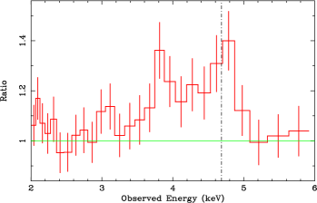
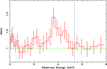
Figure 1: In the top panel, we show the data to model ratio for a model comprising Galactic absorption plus power law. Clear residuals in the form of a double–peaked emission feature are seen in the 3.4-5.1 keV band (4.6–7 keV keV in the rest–frame). In the bottom panel the ratio is relative to a model including one Gaussian emission line at $\sim$ 6.4 keV. The vertical line shows the rest–frame energy of the neutral Fe K$\alpha$ emission line (6.4 keV). Data have been rebinned for visual clarity.

We then add a Gaussian emission line to the simple continuum model. We obtain an improvement of $\Delta\chi^{2}=13$ for 3 degrees of freedom (dof) for a line energy of $6.41\pm 0.17$ keV. Throughout the paper, line energies are given in the rest–frame unless specified otherwise. The line is resolved and has a width of $\sigma=0.28^{+0.41}_{-0.17}$ keV. We measure a line equivalent width of about 150 eV. However, this value has to be corrected because of the galaxy redshift and is about 205 eV at 6.4 keV in the rest–frame. Residuals are still present in the form of a broad emission feature at lower energy, as shown in the bottom panel of Fig. 1. We then add a second Gaussian emission line to account for the lower energy residuals. This improves the statistics by a further $\Delta\chi^{2}=11$ for 3 more free parameters with a final result of $\chi^{2}=281$ for 304 dof. The second Gaussian line is redshifted with respect to 6.4 keV with energy of $5.3\pm 0.2$ keV and is broad ($\sigma=0.4^{+0.7}_{-0.2}$ keV) with respect to the EPIC–pn spectral resolution. The equivalent width of this lower energy line is about 180 eV in the source rest–frame. Now that both lines are included, we re–compute best–fitting parameters and errors and give our final results in Table 1. With the addition of the lower energy broad line, the 6.4 keV emission line becomes consistent with being unresolved (less than 400 eV in width).

We also tested a different continuum model in which the primary continuum is partially covered by a column of gas local to the source. This model is implemented by adding the ZPCFABS model in XSPEC to the power law continuum plus Galactic absorption. The partial covering model has column density ($N_{H}$) and covering fraction ($f_{c}$) of the absorber as free parameters and has the potential of reducing the strength of the broad redshifted emission line (because it induces curvature in the continuum). We also include a $\sim$ 6.4 keV Gaussian emission line. We obtain an acceptable fit ($\chi^{2}=286$ for 305 dof to be compared with $\chi^{2}=281$ for 304 dof for the double Gaussian model). The partial covering parameters are not well constrained with an upper limit on the column density of $N_{H}<2\times 10^{23}$ cm^-2 and a covering fraction between 30 and 95 per cent. Moreover, residuals are still present around 5.3 keV. This is because, the emission at 5.3 keV (see bottom panel of Fig. 1) is more peaked than predicted by a partial coverer. Indeed, the addition of a second Gaussian emission line at 5.3 keV marginally improves the partial covering fit by $\Delta\chi^{2}=6$ for 3 more free parameters. When the second Gaussian is added, the partial covering parameters become totally unconstrained with best–fitting values tending to eliminate any absorber contribution. Therefore, partial covering potentially reduces the significance of the 5.3 keV line but, though not excluded, such a scenario is certainly not required by the data which do prefer a solution in terms of the double Gaussian model. Better quality data are needed to clarify this issue with less ambiguity. In the analysis below we shall consider a simpler continuum model in which the X–ray continuum does not suffer from partial covering complex absorption.

The overall line profile can be better illustrated as follows: we fit the data with the power law continuum model (plus cold absorption with column fixed to the Galactic value), add a Gaussian emission line model, and step on line energy and normalisation in the ranges $4$–$8$ keV and $0$–$2.5\times 10^{-5}$ ph cm^-2 s^-1 respectively. We then record the $\Delta\chi^{2}$ with respect to the original continuum model and compute the confidence contour levels. In Fig. 2, we show the result of this exercise. The contours represent an improvement in $\chi^{2}$ by 4.61, 6.17, 9.21, and 11.8 for two more degrees of freedom (from the outermost to the innermost) and the vertical lines are the best–fitting energies from the double Gaussian model.

3.1 Statistical significance of the redshifted broad line

A narrow iron line at 6.4 keV is ubiquitous in the X–ray spectra of AGNs, and begins to be detected often in quasars as well (Page et al 2004; Yaqoob & Padmanabhan 2004; Jiménez–Bailón et al 2005). In our double Gaussian best–fit model, the width of the 6.4 keV line is unconstrained, and only an upper limit of 400 eV can be computed. The line energy and width are thus consistent with that of neutral Fe K$\alpha$ emission from distant material (torus or broad line region).

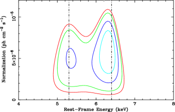
Figure 2: Contours in the flux–energy plane when a Gaussian filter is applied to the data modelled with a power law continuum. The contours represent an improvement in $\chi^{2}$ of 4.61, 6.17, 9.21, 11.8 for the addition of two parameters. The vertical lines are the best–fit energies of the emission lines when a phenomenological double Gaussian model is used.

However, the overall line profile (see top panel of Fig. 1 and Fig. 2) is reminiscent of a double–peaked line profile such as that theoretically expected from the accretion disc and shaped by Doppler and gravitational energy shifts due to high velocity and strong gravity in the vicinity of the central black hole. The detection of a relativistic Fe line from the accretion disc in a radio–loud quasar is much more interesting than that of a narrow Fe line and therefore deserves a detailed significance study. Below, we perform a test on the significance of the broad part of the line profile making use of Montecarlo simulations.

3.1.1 Montecarlo simulations

We carried out a test on the broad line detection significance by extending the method presented by Porquet et al (2004). The pessimistic assumption is that the blue peak at 6.4 keV is completely due to unresolved narrow emission (e.g. reflection from distant matter) and is not part of a relativistic profile. We here test only the significance of the broad part of the line (that modelled by the 5.3 keV Gaussian line in the double Gaussian model). If the overall line profile is due to a relativistic double–peaked line without much contribution from an unresolved component, the test clearly underestimates the significance of the relativistic line and represent a most conservative lower limit.

We use the best–fitting parameters of a power law plus narrow 6.4 keV model as our null hypothesis. The 6.4 keV peak of the line is well reproduced by the model. As throughout the paper, the model includes Galactic absorption with fixed column density. As mentioned, residuals do appear as a broad emission feature at 5.3 keV (bottom panel of Fig. 1) and the purpose of the following exercise is to assess the probability that they are due to noise in the data. The procedure is as follows:

1. starting from the null hypothesis model, we simulate a spectrum with the same exposure as in the data and subtract the appropriate background;

2. the spectrum is fitted with the model used to generate it, and parameters are recorded, providing a new and refined null hypothesis model which differs from the original due to photon statistics only;

3. we use this refined model to generate a simulated spectrum, subtract the appropriate background, fit it with the power law plus narrow 6.4 keV line, and record the $\chi^{2}$. We then add a second Gaussian emission line, vary its energy in the 4–8 keV range, fit the data at each step with line width and normalisation free to vary, and we record the best–fitting parameters and the maximum $\Delta\chi^{2}$;

4. we repeat the above steps 1000 times and obtain the distribution of $\Delta\chi^{2}$, to be compared with the result obtained from the data. The addition of the second Gaussian in the data gives an improvement of $\Delta\chi^{2}=11.4$ with respect to the null hypothesis model.

This procedure gives us an estimate on the significance of the broad red wing of the line under the hypothesis that a narrow 6.4 keV line is present. Moreover, step (ii) ensures that the uncertainty in the null hypothesis is properly taken into account because each spectrum used to compare with the data is obtained from a different realisation of the hypothesis, which differs from the original due to photon counting statistics.

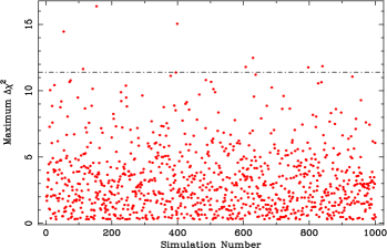
Figure 3: Distribution of the maximum $\Delta\chi^{2}$ obtained when the 1000 simulated spectra are fitted with the null hypothesis model plus an additional Gaussian emission line. The $\Delta\chi^{2}$ is with respect to the null hypothesis fit. The horizontal line is the result obtained by applying the same procedure to the data. Only 9 spectra show evidence for an additional emission line with the same or higher $\Delta\chi^{2}$ as that obtained in the data. Therefore, the broad part of the line seen in the real data is significant at the 99.1 per cent level.

In Fig. 3 we show the measured $\Delta\chi^{2}$ distribution from the 1000 simulated spectra and compare it with the result from the data (horizontal line). The simulations show that the probability to detect a line (broad or narrow) in the whole 4–8 keV band and producing the same (or better) statistics than the broad part of the line in the real data is 9/1000, i.e. the broad part of the line is significant at the 99.1 per cent level. As mentioned, this figure represents the most conservative lower limit for the significance of the relativistic line as a whole.

3.2 Direct spectral fitting

The observed line profile (see Fig. 1 and 2) is very similar to that expected from an accretion disc extending down in the relativistic region close to the black hole. As demonstrated above, the broad part of the line is significant at the 99.1 per cent level. The 6.4 keV peak is however consistent with being unresolved. We then test two different possible scenarios by direct spectral fitting. In the first one, the whole line profile is due to reflection from the accretion disc, while in the second case, we allow a narrow 6.4 keV component to be present.

3.2.1 A single relativistic iron line

Parameter	Blue Line	Red Line
	TWO GAUSSIAN
$E$ (keV)	$6.4\pm 0.2$	$5.3\pm 0.2$
$\sigma$ (eV)	$<400$	$400^{+700}_{-200}$
EW (eV)	$205^{+135}_{-150}$	$180^{+280}_{-110}$
$\chi^{2}/{\rm{dof}}=281/304$
	DISKLINE
$E$ (keV)	–	$6.4^{f}$
$\sigma$ (eV)	–	–
EW (eV)	–	$410^{+240}_{-150}$
$r_{\rm{in}}$ ($r_{g}$)	–	$6^{f}$
$r_{\rm{out}}$ ($r_{g}$)	–	$1000^{f}$
$q$	–	$4.1^{+2.5}_{-1.4}$
$i$ (degrees)	–	$34^{+5}_{-9}$
$\chi^{2}/{\rm{dof}}=282/307$
	GAUSSIAN + DISKLINE
$E$ (keV)	$6.6^{+0.37p}_{-0.2p}$	$6.4^{f}$
$\sigma$ (eV)	$10^{f}$	–
EW (eV)	$<80$	$400^{+300}_{-180}$
$r_{\rm{in}}$ ($r_{g}$)	–	$6^{f}$
$r_{\rm{out}}$ ($r_{g}$)	–	$1000^{f}$
$q$	–	$>2.7$
$i$ (degrees)	–	$<38$
$\chi^{2}/{\rm{dof}}=282/305$

Table 1: Results of the spectral fitting of the hard EPIC–pn spectrum of PG 1425+267 with the different models we explored. Here the symbol ^f means that the parameter has been fixed, while the symbol $p$ denotes that the parameter pegged to the lower and/or higher allowed boundaries. Energies and equivalent widths (EW) are corrected for the galaxy redshift.

The single relativistic line hypothesis can be tested by re–fitting the data with a DISKLINE component only (Fabian et al 1989). The model describes the line profile expected if the Fe line is emitted from the accretion disc around a non–rotating black hole. We keep the energy of the line fixed at 6.4 keV and fix the outer and inner disc radii to $1000~{}r_{g}$ and $6~{}r_{g}$ respectively (as appropriate if the disc extends down to the innermost stable circular orbit). The results of this test are reported in Table 1 and the fit is of the same statistical quality than that with two Gaussian emission lines (which is however more phenomenological than physically motivated). The F–test for the addition of the relativistic line with respect to the power law continuum gives a significance larger than 99.99 per cent. The disc inclination is well constrained ($i=34^{+5}_{-9}$ degrees) and the emissivity profile is only marginally steeper than $q=2.5$.

We also tested if emission from radii smaller than $6~{}r_{g}$ is required by using the LAOR model, appropriate for Kerr black holes (Laor 1991). If so, this would suggest that the black hole is spinning because the accretion disc can extend within $6~{}r_{g}$ only if the spin is different from zero. However, we did not find any conclusive result, with a 90 per cent upper limit on the inner disc radius of $16~{}r_{g}$ (the outer disc radius is fixed at its maximum allowed value of $400~{}r_{g}$). If the emissivity index is fixed at its standard value of $q=3$ the upper limit reduces to $8.5~{}r_{g}$ which is still consistent with a disc around a non–spinning black hole. Thus, we conclude that the data are consistent with any black hole spin from zero to maximal, and that black hole spin is not required by the data.

3.2.2 A narrow and a relativistic broad iron line

To explore the possibility that the 6.4 keV peak of the line is due (or partly due) to the presence of an unresolved narrow component (e.g. from distant matter), we consider a composite model with a narrow Gaussian emission line and a relativistic one. We fix the width of the Gaussian line to 10 eV and retain the DISKLINE model as above. We find a good fit with the same statistical quality as the previous one. However, many of the parameters are unconstrained because of a clear degeneracy. In particular, since the disc inclination is related to the blue horn of the relativistic line, it can not be constrained simultaneously with the narrow Gaussian energy and flux. The same is true for the emissivity index. Therefore the narrow Gaussian energy ranges in all the allowed range (6.4–6.97 keV), its normalisation is only an upper limit, and both the disc emissivity and inclination are measured only as a lower and upper limit respectively. We therefore conclude that some contribution to the blue peak from a narrow Gaussian emission line can not be excluded but is not required by the data.

3.2.3 The reflection continuum

The most likely interpretation is that we are observing Fe emission whose detailed line profile is shaped by special and general relativistic effects in the inner regions of the accretion disc. Since the emission line we observe is a signature of X–ray reflection, we replace the power law continuum with a PEXRAV reflection model (Magdziarz & Zdziarski 1995) with cut–off energy fixed to 100 keV and solar abundances. If the reflector is the accretion disc, as it seems likely from the line profile, the reflection continuum is also broadened and blurred by the relativistic effects. We then apply self–consistently the same relativistic blurring to the line and to the reflection continuum and show in Fig. 4 the confidence contour for photon index and reflection fraction. A reflection continuum is not required by the data, but we cannot exclude it, with a 90 per cent upper limit on the reflection fraction of $\sim$ 1.2. Notice that the inclusion of the reflection continuum does not change the parameters of the relativistic Fe line. With our best–fit DISKLINE model, the (observed–frame) 2–10 keV flux turns out to be $1.6\times 10^{-12}$ erg cm^-2 s^-1, corresponding to a rest–frame luminosity of $6.4\times 10^{44}$ erg s^-1.

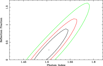
Figure 4: Confidence contour for the (relativistically blurred) reflection fraction and photon index. The contours represent region of 68, 90, and 99 per cent confidence.

4 Short–timescale variability of the line profile?

Time–resolved spectroscopy has the great potential of revealing more clearly the origin of the emission feature. If the Fe line we see in the data is coming from the inner accretion disc, some variability could be present. We then investigate below such a possibility by splitting the observation in different equal duration intervals.

4.1 Splitting the observation in two halves

We split the observation in two equal duration intervals about 24 ks long and subtract from the two spectra the corresponding background. Due to background flares, the net exposure in the two spectra is slightly different and much shorter than 24 ks. We fit the two spectra with the same power law model plus Galactic absorption as above and add Gaussian emission lines if required. We also repeat the procedure used to produce to Fig. 2 and present our results in Fig. 5. We find one significant emission line in the first half of the observation at $6.5\pm 0.2$ keV, while a lower energy line at $5.4\pm 0.3$ keV is detected only marginally. In the second half, two emission lines are clearly detected at $5.1\pm 0.2$ keV, and $6.2\pm 0.3$ keV. The different styles of the vertical lines distinguish between clear and marginal detections.

The line profile appears to be different in the two halves of the observation with the strongest of the peaks seen at $6.5\pm 0.2$ keV in the first half and at $5.1^{+0.2}_{-0.1}$ keV in the second. However, it is clear that claiming variability on firm statistical grounds is a difficult task because emission above the continuum seems to be present at any given energy between 4.8 keV and 6.6 keV in both intervals. In fact the intensity of the stronger line at 5.1 keV in the second half is $8.4^{+6.2}_{-5.4}\times 10^{-6}$ ph cm^-2 s^-1. If a line with the same energy (and width) is fitted to the first half spectrum, we obtain a 90 per cent upper limit of $4.5\times 10^{-6}$ ph cm^-2 s^-1 on its intensity. The two intensities are (though somewhat marginally) consistent with each other, so that no variability can be claimed. A detailed discussion on the significance of the variability is deferred to a shorter timescale analysis below.

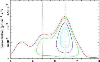
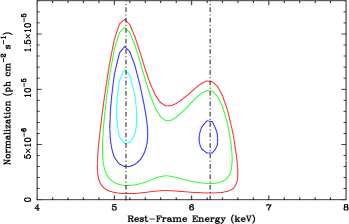
Figure 5: Same as Fig. 2 but for the first half (top) and the second half (bottom) of the observation. The vertical lines are the best–fit energies from the spectral fits with a power law plus Gaussian(s) model. Different line styles are attributed to secure and marginal detections.

         

         

         

         

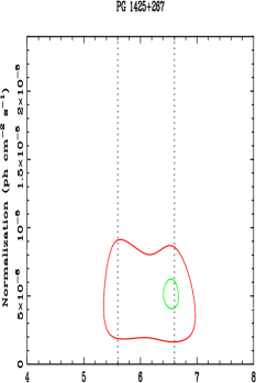
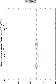
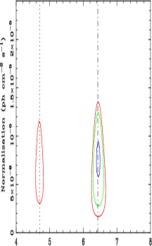
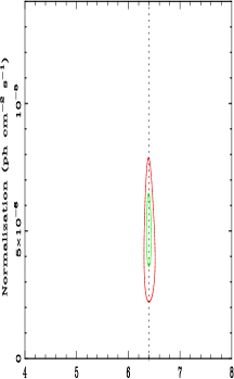
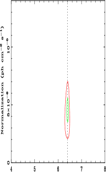
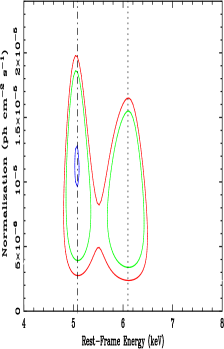
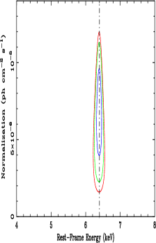
Figure 6: Left Panels: The observation of PG 1425+267 is divided into 4 quarters (about 12 ks total duration each but shorter net exposures). From top to bottom, the evolution of the iron line profile can be seen suggesting dramatic short–timescale variability. Right Panels: Same as in the left panels, but for the quasar PG 1114+445, taken as comparison. The individual spectra have approximately the same number of counts than in the case of PG 1425+267 in the 4–8 keV band and are selected to be contiguous in the observation. Nothing like the variability suggested in PG 1425+267 (see left panels) can be seen.

Here we just mention that, if real, the variation would suggest that different regions of the accretion disc are responsible for the Fe line emission in the two intervals. In particular, the reversal in the prominence of the peaks (from blue to red) is a signature that, in the second half of the observation, emission comes from a more redshifted region of the disc than during the first half, such as a the region on the disc receding from the observer.

4.2 Splitting the observation in four quarters

In order to understand if the tentative variability of the line profile is real we consider a shorter timescale analysis. It is in fact possible that the variability happens at shorter timescales than explored so far and that it is diluted by time–averaging on too long intervals. We then split the observation in four equal duration duration intervals about 12 ks long, and subtract from the four spectra the corresponding backgrounds. Due to randomly distributed background flares, the net exposure in the spectra is not always the same and always shorter than 12 ks (which is the total observation time, not the net exposure). This prevents us to investigate shorter timescales which do not provide good enough quality spectra.

We fit the four spectra separately with the same power law plus Galactic absorption model used for the time–averaged data and add Gaussian emission lines if required. We also repeat the procedure that produced Fig. 2 and present our results in the left panels of Fig. 6. Emission lines are detected in the first, second, and fourth interval. In the third interval, no line is clearly detected. As an indication, we show a low–significance contour representing an improvement in $\chi^{2}$ between 2.3 and 4.61 (for two degrees of freedom).

There is no clear pattern in the evolution shown in the left panels of Fig. 6, except that the blue peak seems to shift to lower and lower energies as time goes on, although the energy shift is significant only from the first ($6.6\pm 0.2$ keV) to the last quarter ($6.1\pm 0.2$ keV). The energy of the blue peak in the last quarter (lower than 6.4 keV considering the 2$\sigma$ errors) excludes that a neutral and constant 6.4 keV Fe line from distant material contributes strongly to the overall line profile. Below 6 keV, the line profile variation appears to be more erratic. This is expected if the line comes indeed from the inner accretion disc. In this case, the blue peak energy is mainly dictated by the observer inclination (the larger the inclination the higher the maximum energy at which the line can be seen), while the red part of the line is more sensitive to the details of the emitting region location on the disc and is expected to vary more erratically.

Before making any comment it is however necessary to estimate the significance of the variations that seem to appear in the different intervals. To do so, we make use once again of Montecarlo simulations. The idea is to see whether the line profile is significantly different in the four spectra.

4.3 Statistical significance of the variability

We first fit jointly the four time intervals spectra with the double Gaussian best–fit model to time–averaged data. The lines parameters are free to vary but forced to be the same in all four intervals while the power law slope and normalisation are allowed to be different in the four intervals (we checked that forcing them to be the same does not change our conclusions). In this way we are testing the goodness of the fit under the hypothesis that the line profile is the same in all intervals (i.e. constant in time) and we record the $\chi^{2}$ for the best–fitting parameters. To test if the line profiles are different in the four intervals (i.e. the line is variable), we then allow the line parameters to vary independently in the four spectra, fit again the data, and record the $\Delta\chi^{2}$ with respect to the previous “constant line profile” fit. We obtain $\Delta\chi^{2}=31.5$ which will be used as a figure for the Montecarlo simulations which are performed as follows:

1. our null hypothesis is now the double Gaussian “constant line profile” best–fit model to the time–averaged spectrum. This is used to generate a time–averaged spectrum which is fitted to obtain a refined null hypothesis which includes the uncertainties due to photon statistics;

2. the new null hypothesis model is used to generate four simulated spectra with the same exposures as the four intervals selected from the real data and appropriate background spectra are subtracted;

3. we fit jointly the four simulated spectra forcing the line parameters to be the same (i.e. forcing the line profile to be constant in time) and record the $\chi^{2}$. We then allow the line profile to be different in the four spectra (i.e. we allow for a variable line profile) and record the $\Delta\chi^{2}$ which is compared to the result obtained on the real data with the same procedure ($\Delta\chi^{2}=31.5$).

The above procedure is repeated 1000 times. In Fig. 7 we show the $\Delta\chi^{2}$ distribution from the simulated spectra and compare it with the result obtained from the data. There are 27/1000 cases in which the resulting maximum $\Delta\chi^{2}$ is as good or better as the result from the data. This means that the line profile variations in the real data are significant at the 97.3 per cent level.

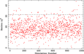
Figure 7: Distribution of the maximum $\Delta\chi^{2}$ obtained when the four simulated spectra are fitted jointly with the double Gaussian model but allowing the line parameters to be different in the four spectra. The $\Delta\chi^{2}$ is computed with respect to the best–fit double Gaussian model in which the line parameters are free to vary, but forced to be the same in the four spectra. The horizontal line is the result obtained with the same procedure on the real data. In 27/1000 cases we find a larger (or equal) $\Delta\chi^{2}$ than in the data, so that the line profile variations in the data are significant at the 97.3 per cent level.

4.4 A plausibility test: the case of PG 1114+445

Here we produce a further test for the line variability with the aim of answering the following question: if the line profile in PG 1425+267 was constant, would the EPIC–pn camera suggest a spurious variability or would it be able to show that the line is indeed not variable? This question has already been answered through Montecarlo simulations. However, we present also a comparison with some real data as a complementary indication.

We searched for a XMM–Newton observation of a PG quasar from the sample collected and analysed by Jiménez–Bailón et al (2005). We were looking for a quasar in which a narrow iron line is detected with the same intensity (or fainter) than the 6.4 keV peak in PG 1425+267 and in which the upper limit on the presence of a relativistic broad line is small. This is because if the iron line is truly narrow and no or little contribution from a broad component is seen, the most likely origin from the line is some distant reflector such as the torus and/or the broad line region and therefore one expects that the line is constant in time. The line must be of the same intensity as in PG 1425+267 to provide a fair comparison.

The best candidate in the sample is PG 1114+445 (z=0.144). In this quasar, Jiménez–Bailón et al (2005) report the presence of a narrow 6.4 keV emission line with equivalent width of $100^{+30}_{-40}$ eV, while the upper limit on a broad component is only $33$ eV (see also Porquet et al 2004a). We downloaded the data from the XSA archive and reduced them using the standard procedures. We here report results from the EPIC–pn detector only. The observation is about 40 ks long. We confirm the detection of a narrow $6.40\pm 0.04$ keV line in the time–averaged spectrum with a rest–frame equivalent width of $140^{+30}_{-60}$ eV. The line is unresolved and the contribution from a broad component (or other fainter peaks) in the whole 4–8 keV band is constrained to be very small (see Fig. 8). Notice that the Fe line in PG 1114+445 has the same intensity ($4.7^{+3.1}_{-2.1}\times 10^{-6}$ ph cm^-2 s^-1) as the 6.4 keV peak in PG 1425+267 ($5.5^{+3.6}_{-4.0}\times 10^{-6}$ ph cm^-2 s^-1), and a slightly smaller rest–frame equivalent width, thereby satisfying our requirements.

As for the more relevant variability study, we selected four consecutive time–intervals in the observation. The exposure in the individual intervals is chosen so that each spectrum has the same number of counts in the relevant 4–8 keV band as the equivalent spectrum obtained when the observation of PG 1425+267 is split into quarters. In this way we make sure that the same photon statistics is reached in the band and the quality of the data is the same. We then repeat the same procedure applied to PG 1425+267 and report the results in the right panels of Fig. 6. We detect a 6.4 keV line in all time–intervals (see Fig 6, right panels). The detection is somewhat marginal in the first three intervals ($\Delta\chi^{2}\leq 9$ for 2 more free parameters), but the presence of an emission feature at the same energy in all intervals is, in our opinion, conclusive.

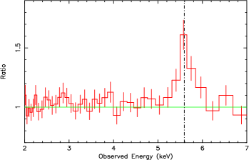
Figure 8: Ratio of the spectrum of PG 1114+445 to a simple power law plus Galactic absorption model. We confirm the detection of a narrow 6.4 keV Fe K$\alpha$ emission line. The iron K$\alpha$ line energy (6.4 keV) is shown in the observed frame as a vertical line. Data have been rebinned for visual clarity.

What the right panels of Fig. 6 show is that, in the case of an emission line with the same intensity of the 6.4 keV peak in PG 1425+267, the XMM–Newton data allow us to detect a constant line, and to rule out any strong variability at the level seen in PG 1425+267 (left panels of the same Figure). No shift in the line energy is seen, contrary to the case of PG 1425+267 and no other emission–like structures do appear in any of the intervals in the whole 4–8 keV band. If the redshifted features seen in PG 1425+267 and the shift in the energy of the 6.4 keV peak were due to noise, it is surprising that we do not detect any of this in the case of PG 1114+445 given that the spectra have the same number of counts. Thus, by comparing the left (PG 1425+267) and right (PG 1114+445) panels of Fig. 6, it seems unlikely that the variability we are suggesting for PG 1425+267 is completely due to noise.

Of course we can not, and do not, consider this simple test as a clear demonstration that the line profile in PG 1425+267 is indeed rapidly variable. However, we report here the result of this straightforward comparison as an additional plausibility argument in favour of the variability, the strict statistical significance of which is established to be at the 97.3 per cent level according to our Montecarlo simulations. Obtaining a better quality long observation of PG 1425+267 with XMM–Newton would allow us to confirm/rule out the short–timescale variability that is tentative and only suggested here, and to apply more sophisticated data analysis techniques (see Iwasawa, Miniutti & Fabian 2004) with the potential of mapping with great accuracy the inner accretion flow in a quasar.

5 Some speculation

Given that the significance of the variability is below 99 per cent, a detailed modelling is not only difficult, but also not recommended. It is however an interesting exercise to try to qualitatively reproduce the apparent variations of the line profile to gain insights on the location of the emitting region. The tentative line profile variations seen in Fig. 5 and 6 suggest that different regions of the accretion disc are responsible for the bulk of the line emission at different times. A succession of relatively short–lived flares illuminating different regions of the disc, one or more orbiting reflecting spots, or disc turbulence/instabilities continuously creating and destroying regions of enhanced emissivity at different locations (e.g. Armitage & Reynolds 2003; Ballantyne, Turner & Young 2005) could well produce the observed line variations. Thus, by fitting the individual line profiles shown in the left panels of Fig. 6 with a model accounting for non–axisymmetric emissivity on the accretion disc, we might be able to infer some information at least on the location of the emitting region in the different time–intervals.

We performed such an analysis by modifying our relativistic line code (Miniutti et al 2003; Miniutti & Fabian 2004), but the parameter space is too large to allow for a unique solution. We can however report that good matches with the observed profiles are obtained by considering emission from one (or two) spot on the disc, always consistent with a radial distance from the black hole of about 6–15 $r_{g}$, but different azimuthal locations in time. It should be noted, merely as an indication, that we never find solutions with very localised spots on the disc, i.e. the radial and, even more dramatically, the azimuthal extent of the emitting region is relatively large ($1~{}r_{g}$ or more and more than 50 degrees, respectively). The large azimuthal extent is unlikely to be due to orbital motion because, the large mass of the black hole in this quasar ($\sim 3\times 10^{9}~{}M_{\odot}$, e.g. Hao et al 2005) implies a typical orbital timescale $\sim$ 250 times longer than that we are exploring here. It is possible that the black hole mass is not very accurate, but it does not seem plausible that it is 100 times smaller than estimated.

The azimuthal extent could be the signature of some elongated structure of enhanced emissivity on the disc such as spiral waves (Karas, Martocchia & Subr 2001). It is also possible that the accretion disc is not geometrically thin (or not completely) and that some elevated regions intercept more efficiently than their surroundings the X–ray illuminating flux coming from the centre. The effect may be strong if the primary X–ray emission comes from very close to the central black hole because, in this case, much of the radiation is beamed along the equatorial plane, so that even small elevations on the disc would make a dramatic difference in the reflection spectrum (see e.g. Miniutti & Fabian 2004).

If elongation due to orbital motion is excluded (see above), and if the variability is associated with changes in the illumination of the disc by flares above it, the extent of the emitting regions can be used to argue against a very small height of the flares above the disc. A flare located at very small height would produce a much smaller spot than observed. This result is in line with what was found in the case of NGC 3516, in which the iron line variability was best explained by a large spot such as that produced by a corotating flare at few $r_{g}$ above the accretion disc (Iwasawa, Miniutti & Fabian 2004).

On the other hand, one large spot can be successfully reproduced by considering a large number of small height flares occurring close to each other in one main region. Notice that a large number of independent flares would violate the log–normal distribution of fluxes that is inferred for both AGN and Galactic BHC from the observed rms–flux relation (Uttley, McHardy 2001; Uttley, McHardy & Vaughan 2005). Indeed, the log–normal distribution strongly argues against the presence of more than 2–3 independent flares. Therefore, if we persist to interpret the emitting regions as due to flares above the disc (rather than structures on the disc itself, independently of the illumination), we can retain only two possibilities: i) one (or two) independent flares are located at a relatively large height (few gravitational radii) above the disc, or ii) a large number of localised, small–height flares occur close to each other in one (or two) main independent regions, but the individual flares in each region are not independent.

It is interesting to note that the “thundercloud model” proposed by Merloni & Fabian (2001) seems to lie in between the two cases. In this model, magnetic flares produce the X–ray continuum via inverse Compton scattering of soft seed photons. The difference with other similar models is that the fundamental heating event must be compact, with size comparable to the disc thickness, but height at least one order of magnitude larger. Moreover, the heating event (most likely due to magnetic reconnection) is shown to proceed in correlated trains (such as in an avalanche) with the size of the avalanche determining the size and luminosity of the overall active region. If the number of simultaneous independent active regions is limited (and only one or two regions are required by the data) the model seems able to reproduce the variability we are suggesting here, potentially preserving at the same time the rms–flux relation and log–normal distribution of fluxes.

6 The broadband spectrum and warm absorber of PG 1425+267

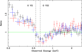
Figure 9: Data to model ratio for the three EPIC detectors when the hard pn model is extrapolated in the soft band. The deficit above 0.5 keV (0.683 keV in the rest–frame) is the signature of absorption by warm photoionized gas. We also show as vertical lines the energies of the expected oxygen edges in the observed frame.

To better constrain the soft spectrum of PG 1425+267, we extracted the MOS spectra as well. If the model we used so far is extended to the soft band, a clear deficit remains in the 0.5–1 keV band (observed frame), most likely due to intervening absorption in a warm absorber (see Fig. 5 in which the extension to the soft spectrum is shown for all XMM–Newton X–ray detectors). Extending the pn data below 0.5 keV is however not recommended because of some residual calibration problems that still affect the pn camera below that energy. Therefore, we used the pn data in the 0.5–8.5 keV range only, while the MOS data are used in the 0.2–8.5 keV (observed energy ranges). With the addition of one absorption edge, the fit is acceptable ($\chi^{2}=1044$ for 939 degrees of freedom). However, the energy of the edge is $0.79\pm 0.03$ keV, which is not consistent with either O VII ($0.74$ keV) nor O VIII ($0.87$ keV), and the depth is very large ($\tau=0.8\pm 0.1$). This probably indicates the simultaneous presence of two edges at energies below and above that measured. We then add a second edge, and fix both energies at the rest–frame values for O VII and O VIII. With this two–edges model, we find an improvement of $\Delta\chi^{2}=16$ for the same number of degrees of freedom with respect to the single–edge model. The depth of the edges are $\tau_{\rm OVII}=0.5\pm 0.2$ and $\tau_{\rm OVIII}=0.4\pm 0.2$. If the energy of the edges are free to vary, they tend to slightly higher values, but are still consistent with the rest–frame energies within the errors. Very little soft excess is present in the MOS data. However, the addition of a (redshifted) blackbody component results in a further improvement in the fit (at more than the 99 per cent level according to the F–test). The temperature of the thermal emission component is $80\pm 10$ eV, cooler than the typical temperature found by Porquet et al (2004a) and Piconcelli et al (2005) in their analysis of the XMM–Newton sample of PG quasars (about $150$ eV). The final power law slope is $\Gamma=1.55\pm 0.03$ and the overall fit is excellent with $\chi^{2}=1004$ for 937 degrees of freedom.

7 Conclusions

The hard spectrum of PG 1425+267 is characterised by the presence of an emission feature which is best described by a double–peaked Fe line profile. The blue peak of the line is consistent with an energy of 6.4 keV and an unresolved width, and its origin could well be in some distant reflector. The red peak of the line (at 5.3 keV) is however redshifted and broad therefore suggesting emission from the accretion disc. According to Montecarlo simulations, the broad and redshifted part of the line profile is significant at the 99.1 per cent level. The simplest interpretation of the time–averaged data is that the accretion disc is acting as a reflector producing an iron K$\alpha$ line whose profile is dictated by Doppler and gravitational shifts in the orbiting gas. The best–fitting model we find is that of a relativistic line from an accretion disc around a Schwarzschild black hole providing a statistical improvement with respect to a simple power law model which is significant at more than the 99.99 per cent level (F–test). No black hole spin is required by the data, although emission from within the marginal stable orbit of a non–rotating black hole cannot be excluded. Due to the quality of the data, it is not possible to exclude a partial covering model plus narrow 6.4 keV line as an alternative to the relativistic line. However, the partial covering model is largely unconstrained and is not able to well reproduce the broad emission feature at 5.3 keV, suggesting that the relativistic line is a better explanation of the hard spectrum. The detection of a broad relativistic line in a radio–loud quasar argues against a scenario in which, due e.g. to low mass accretion rate, the disc in such objects is truncated (see also the discussion in Ballantyne & Fabian 2005).

When the observation is split into quarters, the energy of the blue peak appears to shift from $6.6\pm 0.2$ keV (first quarter of the observation) to $6.1\pm 0.2$ keV (last quarter) in less than 48 ks. The fast variability and the energy of the blue peak in the last quarter excludes a strong contribution to the line profile from a constant 6.4 keV iron line from distant material. The large majority (if not all) of the line profile is therefore likely emitted from a highly dynamical medium such as the accretion disc. Moreover bright redshifted peaks appear at $4.7\pm 0.2$ keV and, with higher significance, at $5.1^{+0.1}_{-0.2}$ keV in the second and last quarter of the observation respectively. We performed simulations to establish the significance of the apparent variations in the line profile and found that they are significant at the 97.3 per cent level.

If the variability is real, it indicates emission from different regions on the accretion disc at different times in a range of 6–15 $r_{g}$ from the central black hole. Our understanding of the inner accretion flow in PG 1425+267 would benefit very much from a future, long, and better quality XMM–Newton observation that would allow us to secure (or rule out) any variability on firm statistical grounds. It is clear (also from previous recent results, see Iwasawa, Miniutti & Fabian 2004 for the remarkable case of NGC 3516) that the potential of future missions with much larger collecting area than XMM–Newton in the Fe K band, such as XEUS and Constellation–X, is outstanding. The prospects of probing the strong gravity regime of General Relativity via X–ray observations of relativistic Fe lines and of their short timescale variability look stronger now than ever before.

References

- Armitage & Reynolds (2003) Armitage P.J., Reynolds C.S., 2003, MNRAS, 341, 1041
- Ballantyne, Turner & Young (2005) Ballantyne D.R., Turner N.J., Young A.J., 2005, ApJ, 619, 1028
- Ballantyne & Fabian (2005) Ballantyne D.R., Fabian A.C., 2005, ApJ, 622, L100
- Brandt, Laor & Wills (2000) Brandt W.N., Laor A., Wills B.J., 2000, ApJ, 528, 637
- Dovčiak et al (2004) Dovčiak M., Bianchi S., Guainazzi M., Karas V., Matt G., 2004, MNRAS, 350, 745
- Fabian et al (1989) Fabian A.C., Rees M.J., Stella L., White N.E., 1989, MNRAS, 238, 729
- Fabian et al (2002) Fabian A.C. et al, 2002, MNRAS, 335, L1
- Fabian et al (2004) Fabian A.C., Miniutti G., Gallo L., Boller Th., Tanaka Y., Vaughan S., Ross R.R., 2004, MNRAS, 353, 1071
- Fabian & Miniutti (2005) Fabian A.C., Miniutti G., 2005, review paper to appear in “Kerr Spacetime: Rotating Black Holes in General Relativity”, eds. D.L. Wiltshire, M. Visser, S.M. Scott, Cambridge Univ. Press, astro-ph/0507409
- Guainazzi (2003) Guainazzi M., 2003, A&A, 401, 903
- Hao et al (2005) Hao C.N., Xia X.Y., Mao S., Wu H., Deng Z.G., 2005, ApJ, 625, 78
- Iwasawa et al (1999) Iwasawa K., Fabian A.C., Young A.J., Inoue H., Matsumoto C., 1999, MNRAS, 306, L19
- Iwasawa, Miniutti & Fabian (2004) Iwasawa K., Miniutti G., Fabian A.C., 2004, MNRAS, 355, 1073
- Jimenez et al (2005) Jiménez–Bailón E., Piconcelli E., Guainazzi M., Schartel N., Rodríguez–Pascual P.M., Santos–Lleó M., 2005, A&A, 435, 449
- Karas, Matocchia & Subr (2001) Karas V., Martocchia A., Subr L., 2001, PASJ, 53, 189
- Laor (1991) Laor A., 1991, ApJ, 376, 90
- Laor et al (1997) Laor A., Fiore F., Elvis M., Wilkes B.J., McDowell J.C., 1997, ApJ, 477, 93
- Longinotti et al (2004) Longinotti A.L., Nandra K., Petrucci P.O., O’Neill P.M., 2004, MNRAS, 355, 929
- Magdziarz &Zdziarski (1995) Magdziarz P., Zdziarski A.A., 1995, MNRAS, 273, 837
- Merloni & Fabian (2001) Merloni A., Fabian A.C., 2001, MNRAS, 328, 958
- Miller et al (2002) Miller J.M. et al, 2002, ApJ, 570, L69
- Miniutti et al (2003) Miniutti G., Fabian A.C., Goyder R., Lasenby A.N., 2004a, MNRAS, 344, L22
- Miniutti & Fabian (2004) Miniutti G., Fabian A.C., 2004, MNRAS, 349, 1435
- Miniutti, Fabian & Miller (2004) Miniutti G., Fabian A.C., Miller J.M., 2004c, MNRAS, 351, 466
- Nandra et al. (1997) Nandra K., Mushotzky R.F., Yaqoob T., George I.M., , Turner T.J., 1997, MNRAS, 284, L7
- Nayakshin & Kazanas (2001) Nayakshin S., Kazanas D., 2001, ApJ, 553, 885
- Page et al (2004) Page K.L., O’Brien P.T., Reeves J.N., Turner M.J.L., 2004, MNRAS, 347, 316
- Petrucci et al (2002) Petrucci P.O. et al, 2002, A&A, 388, L5
- Piconcelli et al (2005) Piconcelli E., Jiménez–Bailón E., Gaunazzi M., Schartel N., Rodríguez–Pascual P.M., Santos–Lleó M., 2005, A&A, 432, 15
- Porquet et al (2004a) Porquet D., Reeves J.N., O’Brien P., Brinkmann W., 2004a, A&A, 422, 85
- Porquet et al (2004) Porquet D., Reeves J.N., Uttley P., Turner T.J., 2004b, A&A, 427, 101
- Reeves & Turner (2000) Reeves J.N., Turner T.J., 2000, MNRAS, 316, 234
- Ruszkowski (2000) Ruszkowski M., 2000, MNRAS, 315, 1
- Schartel et al (2005) Schartel, N., Rodríguez-Pascual P.M., Santos-Lleó M., Clavel J., Guainazzi M., Jiménez-Bailón E., Piconcelli E., 2005, A&A, 433, 455
- Tanaka et al (1995) Tanaka Y. et al, Nature, 375, 659
- Turner et al. (2002) Turner T.J. et al., 2002, ApJ, 574, L123
- Turner, Kraeme & Reeves (2004) Turner T.J., Kraemer S.B., Reeves J.N., 2004, ApJ, 603, 62
- Uttley & McHardy (2001) Uttley P., McHardy I.M., 2001, MNRAS, 323, L26
- Uttley, McHardy & Vaughan (2005) Uttley P., McHardy I.M., Vaughan S., 2005, MNRAS, 359, 345
- Wilms et al (2001) Wilms J., Reynolds C.S., Begelman M.C., Reeves J., Molendi S., Staubert R., Kendziorra E., 2001, MNRAS, 328, L27
- Yaqoob et al. (2003) Yaqoob T., George I.M., Kallman T.R., Padmanabhan U., Weaver K.A., Turner T.J., 2003, ApJ, 596, 85
- Yaqoob & Padmanabhan (2004) Yaqoob T., Padmanabhan U., 2004, ApJ, 604, 63