Behavior of Torsional Alfven Waves and Field Line Resonance on Rotating Magnetars

Abstract

Torsional Alfven waves are likely excited with bursts in rotating magnetars. These waves are probably propagated through corotating atmospheres toward a vacuum exterior. We have studied the physical effects of the azimuthal wave number and the characteristic height of the plasma medium on wave transmission. In this work, explicit calculations were carried out based on the three-layered cylindrical model. We found that the coupling strength between the internal shear and the external Alfven modes is drastically enhanced, when resonance occurs in the corotating plasma cavity. The spatial structure of the electromagnetic fields in the resonance cavity is also investigated when Alfven waves exhibit resonance.

1 Introduction

Soft gamma-ray repeaters (SGRs) and anomalous X-ray pulsars (AXPs) have been known as strongly magnetized neutron stars, magnetars. The hallmark of these objects is to repeat X-ray or gamma-ray emissions irregularly. So far, four or five known active objects which show frequent X-ray emission of tremendously energetic and shorter initial bursts (typically $E\lesssim 10^{41}$ ergs and $\Delta t\sim 0.5$ s) have been identified with SGRs (Thompson et al. 2001). Some of them occasionally exhibit more energetic events. The giant flare 1900+14, now associated with SGR 0525-66, was observed in 1979 (Mazets, Golenetskii, and Gur’yan 1979) for the first time and became active again in 1992 (Kouveliotou et al. 1993) and also in 1998 (Kouveliotou et al. 1998 ; Hurley et al. 1999). Recently, the intense $\gamma$-ray flare from SGR 1806-20 occured on December 27, 2004 was reported (Palmer et al. 2005; Hurley et al. 2005; Mereghetti et al. 2005). Rea et al. (2005) have investigated the pulse profile and flare spectrum of SGR 1806-20. Their study may potentially give the information about the global field structure in the magnetosphere and may further promote theoretical magnetar models. Their extream peak luminosity extends up to $10^{6}L_{\text{Edd}}$ estimated at a distance of 10 kpc (Mazets et al. 1999; Feroci et al. 2001). Typical X-ray luminosities of SGRs have been measured to be $L_{\text{x}}=10^{34}$-$10^{36}$ erg s^-1 (Hurley et al. 2000; Thompson et al. 2000), except with giant bursts SGRs 1900+14 and 1806-20. Shorter durations of initial flares of SGRs are comparable to the Alfven crossing time of the core. The energy distribution shows good agreement with Gutenberg-Lichter law, which may indicate statistical similarity to earthquakes or solar flares (Cheng et al. 1996; Gogus et al. 1999, 2000). The SGRs have spin periods in a small range of $P=5$-$8$ s with rapid spin down rate $\dot{P}\simeq 10^{-10}$ ss^-1 , which therefore give characteristic ages $P/\dot{P}\sim$ $10^{3}$ yr (Mazets et al. 1979; Kouveliotou et al. 1998; Hurley et al. 1999a).

On the other hand, the physical nature of AXPs is still uncertain due to poor observations, but there seem to be some similarities and differences between SGRs and AXPs. AXPs are energetic sources of pulsed X-ray emission, whose periods lie in a narrow range $P=6$-$12$ s, characteristic ages $P/\dot{P}=$ $3\times 10^{3}\sim 4\times 10^{5}$ yr and X-ray luminosities $L_{\text{x}}=5\times 10^{34}$-$10^{36}$ erg s^-1(Mereghetti 2000; Thompson 2001). AXP sources likely have somewhat larger active ages and some of them have softer X-ray spectra compared with SGRs. One of the primary difference between them will be that AXPs so far have shown only quiescent X-ray emission with no bright active bursts such as giant flares. Active ages of SGRs and AXPs are consistent with the observed evidence that these compact objects often give their location close to the edge of shell-type supernova remnants. Neither SGRs nor AXPs show the presence of conspicuous counterparts at other wavelengths (Mereghetti & Stella 1995; Mereghetti et al. 2002). Origin of these enourmous energetics is likely to come from their strong magnetic fields $B=10^{14}$-$10^{15}$ G estimated by their spin periods and spin down rates. Only the magnetar model has been able to account for the enigmatic properties of a rare class of SGRs or AXPs.

Shear and Alfvenic waves play an essential role on the energy transfer to the exterior in the burst-like phenomena observed in SGRs or giant flares. The Alfven wave propagation in such a strongly magnetized star should be clarified theoretically. In our previous work, the propagation and transmission of torsional Alfven waves have been studied, focused only on the fundamental mode of azimuthal wave number $m=1$ as a first step. In that work, the exterior of the star is examined qualitatively only, assuming two extreme cases: (i) corotating together with the star and (ii) static state independent of the stellar rotation. The former will come true when the plasma gas is trapped by closed magnetic field lines, and the latter will be realized without any other force. In any case, it might be inadequate at least in the following two points to place such strong constraints on the wave mode and on ambient circumstances of the star in the previous paper. First, under the more realistic situations various modes with azimuthal wave number $m\gg 1$ are probably triggered by star quake. Second, it is natural to assume that a scale height of the plasma gas is neither $L=0$ nor $L\rightarrow\infty$, but has a finite value of $L$. Huang et al. (1998) pointed out that a relativistic fireball like those in classical GRBs may exist in SGRs. Recently, Thompson and Duncan (2001) have also suggested that after the initial hard spike emission, some lumps of hot plasma gas involving electron-positron pairs and high energy photons, that is, fireball, would be created on closed magnetic field lines. In fact, the fast decline and complete evaporation on X-ray light curve observed in the August 27 burst provides a clear evidence of the trapped fireball. Motivated by this, we thus extend our study to include some plasma gas spreading over the stellar surface.

The main aim of this paper is to study the physical behavior of the torsional Alfven waves with azimuthal wave number $m$ in the presence of corotating plasma confined within a certain finite distance $L$ and then to investigate the effects of these quantities $m$ and $L$ on the wave propagation and transmission. In section 2, our model is self-consistently constructed and the relevant basic equations are formulated. These equations are almost the same as those derived in Kojima and Okita (2004), but are summarized here for the paper to be self-contained. In section 3, we shall derive the dispersion relation in a WKB way to show that the rotating plasma atmosphere plays a crucial role as a resonant cavity of the wave when a certain condition holds. In section 4, transmission rates of the Alfven waves are numerically calculated. In section 5, their electromagnetic field structure is also discussed with the numerical results. In section 6, we give a brief summary of our findings and their implications for the torsional Alfven waves on rotating magnetars.

2 Electromagnetics on Rotating Magnetars

2.1 Model

Both the magnetic field and the rotation of star lead to a complicated geometrical configuration. In this paper we assume some simplified conditions to understand the physical processes of the wave propagation. We here consider three-layered cylindrical model with radius $\varpi_{\text{pc}}$. It is composed of the neutron star crust between $z=-q$ and $z=0$ (region (1)), corotating plasma above the stellar surface between $z=0$ and $z=L$ (region (2)) and static pure vacuum at $z>L$ (region (3)) as shown in Fig.1. The plasma gas filled in the atmosphere corotates with the crust at the same angular velocity $\Omega$. Local magnetic fields permeate uniformly in each layer and point along the $z$ direction, $\mathbf{B}=B_{\text{o}}\mathbf{e}_{z}$, which represents open magnetic fields extending to infinity.

Alfven waves excited at the bottom of the crust $q\approx 10^{5}$ cm owing to some mechanisms, travel upward along the local magnetic field lines. They are partially reflected and transmitted at the boundaries $z=0$ and $z=L$, where the physical property of Alfven waves significantly changes because of the effect of the background rotation, as shown below. This model, by setting $L\rightarrow\infty$, reduces to the case in which the plasma gas extends infinitely to the exterior of the star, while setting $L\rightarrow 0$ reduces to the simple case in which the exterior is filled with pure vacuum only. Up to the present time, we have no observational information of the plasma size $L$. In this work, $L$ is regarded as a free parameter in order to investigate its effect on the wave propagation and transmission.

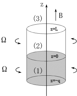
Figure 1: Three-layered cylindrical model. Region (1) corresponds to the rotating neutron star crust with a constant angular velocity $\Omega$, region (2) corresponds to the fireball as a resonant cavity filled with plasma corotating with $\Omega$, and region (3) denotes a static pure vacuum.

We shall now give some comments on the validity of this model by comparing the physical sizes $\varpi_{\text{pc}}$, $q$ and $L$ with the stellar radius $R$. In this model we have explicitly assumed that the local magnetic field has a $z$-component only. Our model can be applied to the polar cap region, whose cylindrical radius $\varpi_{\text{pc}}$ is given by $\varpi_{\text{pc}}=R\sin\theta_{\text{pc}}\approx 10^{4}\left(T/1\text{s}\right)^{-1/2}$ cm $\ll$ $R=10^{6}$ cm. Curvature of the stellar surface and the magnetic field lines may be neglected within the polar cap region. In a similar way, it may be valid to assume that the local magnetic field lines are uniform if the thickness of each layer is smaller than the star radius, $L,q\ll R$. We can also extend our model to the extreme case $L\sim R$. Even in this case, the validity of this model nevertheless holds good near the z-axis. In the remainder of this paper we ristrict our explicit calculations only to the axially symmetric small region within the polar cap radius, unless otherwise stated.

2.2 Linear Perturbation

In this section, we consider the propagation of torsional shear-Alfven waves with various azimuthal modes on rotating magnetars. Such waves are probably excited by the turbulent motion of the starquake in the deep crust, but above the neutron drip $(z>z_{\text{nd}}\approx-10^{5}$ cm$)$. Many proposals for starquake model have been put forward (e.g., Pacini and Ruderman 1974), but all of them are generally argued only for weakly magnetized neutron stars with $10^{11}-10^{12}$ G. Therefore, their treatments are inadequate for magnetars, as they are. However, analogous mechanism may also occur in magnetars. In this paper, we do not discuss the triggering mechanism of the starquake itself, but focus only on the process by which electromagnetic shear waves, once generated, are propagated and transmitted from the deep crust, through a magnetized plasma, toward the vacuum exterior.

We assume that the horizontal Lagrange displacement $\mathbf{\xi}=(\xi_{\varpi},\xi_{\phi},0)$ is suddenly shaken in the deep interior at depth $q\approx 10^{5}$ cm, nevertheless the matter remains immobile in the vertical direction due to strong gravity of the neutron star, $g\sim 10^{14}$ cm s^-2. Therefore the following transverse wave condition may be easily satisfied.

$$\nabla\cdot\mathbf{\xi=}\dfrac{1}{\varpi}\dfrac{\partial}{\partial\varpi}\left(\varpi\xi_{\varpi}\right)+\dfrac{1}{\varpi}\dfrac{\partial\xi_{\phi}}{\partial\phi}=0.$$ (1)

As one of the simplest solutions, wave ansatz under this condition can be written formally as

$$\mathbf{\xi}(\varpi,\phi,z,t) =\left(\mathbf{e}_{\varpi}\pm i\mathbf{e}_{\phi}\right)\left(\dfrac{\varpi}{\varpi_{\text{pc}}}\right)^{m-1}\xi_{\pm m,\omega}\left(z\right)e^{-i\left(\omega t\mp m\phi\right)}\text{ }$$

$$(m =1,2,3\cdots).$$ (2)

Here notation ‘$\pm$’ denotes the difference of helicity states. Displacements and other perturbed quantities are always assumed to have a harmonic time dependency $e^{-i\omega t}$.

The crust and the surrounding plasma can be regarded as a perfect conductor because ohmic dissipation timescales are very long compared with other timescales of interest. The frozen condition can read

$$\mathbf{E+}\dfrac{1}{c}\mathbf{v}\times\mathbf{B=}0.$$ (3)

Background is assumed to rotate uniformly with $\mathbf{v}=\varpi\Omega\mathbf{e}_{\phi}$, which means that the local electric field arround a highly conducting spherical star has only a radial component $\mathbf{E}=(-\varpi\Omega B_{\text{o}}/c)\mathbf{e}_{\varpi}$. The electric field now generates the Goldreich-Julian charge density

$$\rho_{\text{e}}=\nabla\cdot\mathbf{E}/4\pi=-\Omega B_{\text{o}}/2\pi c.$$ (4)

Transverse displacements of the crustal matter produce electromagnetic field perturbations propagating along the local magnetic field $\mathbf{B}=B_{\text{o}}\mathbf{e}_{z}$. A self-consistent set of Maxwell’s equations for perturbed electromagnetic fields $\delta\mathbf{E}$ and $\delta\mathbf{B}$ are

$$\nabla\cdot\delta\mathbf{E}=4\pi\delta\rho_{\text{e}},$$ (5)

$$\nabla\cdot\delta\mathbf{B}=0,$$ (6)

$$\nabla\times\delta\mathbf{E}=-\dfrac{1}{c}\partial_{t}\delta\mathbf{B},$$ (7)

$$\nabla\times\delta\mathbf{B}=\dfrac{4\pi}{c}\delta\mathbf{j}+\dfrac{1}{c}\partial_{t}\delta\mathbf{E,}$$ (8)

where $\delta$ denotes Eulerian perturbation. By taking the perturbation of equation (3) and then combining with equation (7), $\delta\mathbf{E}$ and $\delta\mathbf{B}$ are expressed as

$$\delta\mathbf{E} =-\dfrac{1}{c}\left(\delta\mathbf{v}\times\mathbf{B}+\mathbf{v}\times\delta\mathbf{B}\right),$$ (9)

$$\delta\mathbf{B} =\left(\mathbf{B}\cdot\nabla\right)\mathbf{\xi.}$$ (10)

By using the relation between the displacement and the velocity perturbation $\delta\mathbf{v}=\partial_{t}\mathbf{\xi}+\left(\mathbf{v}\cdot\nabla\right)\mathbf{\xi}-\left(\mathbf{\xi}\cdot\nabla\right)\mathbf{v}$ together with equation (2), one obtains

$$\delta\mathbf{E} =\dfrac{B_{\text{o}}}{c}\left(\dfrac{\varpi}{\varpi_{\text{pc}}}\right)^{m-1}$$

$$\times\left[\mp\left(\omega\mp m\Omega\right)\xi_{\pm}\left(\mathbf{e}_{\varpi}\pm i\mathbf{e}_{\phi}\right)+\Omega\varpi\dfrac{d\xi_{\pm}}{dz}\mathbf{e}_{z}\right]e^{-i\left(\omega t\mp m\phi\right)},$$ (11)

$$\delta\mathbf{B} =B_{\text{o}}\left(\dfrac{\varpi}{\varpi_{\text{pc}}}\right)^{m-1}\dfrac{d\xi_{\pm}}{dz}\left(\mathbf{e}_{\varpi}\pm i\mathbf{e}_{\phi}\right)e^{-i\left(\omega t\mp m\phi\right)}.$$ (12)

Equations (11) and (12) imply that if stellar rotation can be completely ignored, then $\delta\mathbf{E}$, $\delta\mathbf{B}$ and the propagation vector $\mathbf{k}=k\mathbf{e}_{z}$ form a mutually orthogonal set of vectors, say, TEM modes. However, in the presence of rotation, such an orthogonality breaks down and thus longitudinal modes of the perturbed electric fields and currents are excited (TM modes). Other perturbed quantities related to the displacement are calculated by using above the results (11) and (12)

$$\delta\mathbf{j} =\dfrac{c}{4\pi}\nabla\times\delta\mathbf{B}-\dfrac{1}{4\pi}\partial_{t}\delta\mathbf{E}$$

$$=\mp i\dfrac{cB_{\text{o}}}{4\pi}\left(\dfrac{\varpi}{\varpi_{\text{pc}}}\right)^{m-1}\times$$

$$\left[\left\{\dfrac{d^{2}\xi_{\pm}}{dz^{2}}+\dfrac{\omega\left(\omega\mp m\Omega\right)}{c^{2}}\xi_{\pm}\right\}\left(\mathbf{e}_{\varpi}\pm i\mathbf{e}_{\phi}\right)\mp\dfrac{\omega\Omega\varpi}{c^{2}}\dfrac{d\xi_{\pm}}{dz}\mathbf{e}_{z}\right]$$

$$\times e^{-i\left(\omega t\mp m\phi\right)},$$ (13)

$$\delta\rho_{\text{e}} =\dfrac{1}{4\pi}\nabla\cdot\delta\mathbf{E}$$

$$=\dfrac{B_{\text{o}}\Omega\omega}{4\pi c}\left(\dfrac{\varpi}{\varpi_{\text{pc}}}\right)^{m-1}\dfrac{d^{2}\xi_{\pm}}{dz^{2}}e^{-i\left(\omega t\mp m\phi\right)}.$$ (14)

The linearized equation of motion for uniformly rotating background from a static equilibrium state governing the torsional Alfven waves is now given by

$$\rho\left[\partial_{t}\delta v_{i}+\left(\mathbf{v}\cdot\nabla\right)\delta v_{i}+\left(\delta\mathbf{v}\cdot\nabla\right)v_{i}\right]$$ (15)

$$= \delta S_{i}+\delta F_{i}+\left(\mathbf{g}\delta\rho\right)_{i}-\left(\nabla\delta p\right)_{i}\quad(i=\varpi,\phi,z).$$

Profile of the mass density $\rho$ in the crust is obtained by solving the equation of state for degenerate electrons as follows (Blaes et al. 1989)

$$\rho =\dfrac{\left(\mu_{\text{e}}m_{\text{u}}\right)^{5/2}}{3\pi^{2}\hbar^{3}}\left(\dfrac{g^{2}\mu_{\text{e}}m_{\text{u}}}{c^{2}}z^{2}+2gm_{\text{e}}\left|z\right|\right)^{3/2}$$

$$\approx 8.0\times 10\left[\left(\dfrac{\left|z\right|}{\text{cm}}\right)+2.5\times 10^{-4}\left(\dfrac{\left|z\right|}{\text{cm}}\right)^{2}\right]^{3/2}\text{g cm}^{-3}\text{,}$$ (16)

where $m_{\text{u}}$ is an atomic mass unit, $\mu_{\text{e}}$ is the mean molecular weight per electron and others have usual physical meanings.

The first term of RHS in equation (15), $\delta S_{i}$, is a perturbed elastic stress tensor associated with distorted matter in the crust and can be written in terms of $\xi$

$$\delta S_{i} =\nabla_{j}\left[\left(\varkappa-\dfrac{2\mu}{3}\right)\delta_{ij}\nabla\cdot\mathbf{\xi}\right]+\nabla_{j}\left[\mu\left(\dfrac{\partial\xi^{i}}{\partial x_{j}}+\dfrac{\partial\xi^{j}}{\partial x_{i}}\right)\right]$$

$$\quad(i,j =\varpi,\phi,z),$$ (17)

where $\varkappa$ is a bulk modulus, $\mu$ is a shear modulus given by

$$\mu =0.295Z^{2}e^{2}n_{i}^{4/3}$$

$$\approx 4.8\times 10^{27}\left(\dfrac{\rho}{10^{11}\text{ g cm}^{-3}}\right)^{4/3}\text{ erg cm}^{-3},$$ (18)

with the ion number density $n_{i}=\rho/Z\mu_{\text{e}}m_{\text{u}}$ and $\delta_{ij}$ Kronecker’s delta. In the following calculations, $Z=32$ will be adopted as a typical value in the crust. If one considers the complete transverse oscillation mode, the first term of equation (17) vanishes owing to $\nabla\cdot\mathbf{\xi}=0$.

The second term on RHS of equation (15) can be resolved into perturbations of Lorentz and Coulomb forces

$$\delta\mathbf{F} =\delta\rho_{\text{e}}\mathbf{E+}\rho_{\text{e}}\delta\mathbf{E+}\dfrac{1}{c}\left(\delta\mathbf{j}\times\mathbf{B+j}\times\delta\mathbf{B}\right)$$

$$\simeq\dfrac{1}{c}\left(\delta\mathbf{j-}\rho_{\text{e}}\delta\mathbf{v}\right)\times\mathbf{B.}$$ (19)

Here we used equation (9) and unperturbed current $\mathbf{j=}\rho_{\text{e}}\mathbf{v}$ induced by the background rotation. We further dropped the term $\delta\rho_{\text{e}}\mathbf{E}\propto\left(\Omega\varpi/c\right)^{2}$, which is small near the z-axis or within the actual stellar radius $R$. Eliminating $\delta\mathbf{j}$ with the help of equation (8), the electromagnetic force reduces to

$$\delta\mathbf{F}\simeq\dfrac{1}{4\pi}\left(\mathbf{B}\cdot\nabla\right)^{2}\mathbf{\xi}-\dfrac{B_{\text{o}}^{2}}{4\pi c^{2}}\partial_{t}\delta\mathbf{v}.$$ (20)

The first term in equation (20) implies the tension of the perturbed magnetic field, while the second one shows the magnetic pressure generated by the distorted matter.

The last two terms of equation (15) represent gravitational force $\left(\mathbf{g}\delta\rho\right)_{i}$ and pressure gradient $\left(\nabla\delta p\right)_{i}$, respectively. However, unless one takes the p- or f-mode such as compressional waves and/or sonic waves into consideration, one can ignore them for simplicity in this model.

2.3 Wave Equation

We shall now derive the wave equation in region (1) shown in Fig.1. Substituting equations (17) and (20) into equation of motion (15), one can obtain the following differential wave equation in terms of the displacement $\xi_{\pm}^{(1)}$

$$\dfrac{d^{2}\xi_{\pm}^{(1)}}{dz^{2}}+\dfrac{1}{\widetilde{\mu}}\dfrac{d\widetilde{\mu}}{dz}\dfrac{d\xi_{\pm}^{(1)}}{dz}+\dfrac{\widetilde{\rho}}{\widetilde{\mu}}\sigma_{\pm}\left[\sigma_{\pm}\pm\left\{m(1-h)+2\right\}\Omega\right]\xi_{\pm}^{(1)}=0,$$ (21)

where $\widetilde{\mu}$ and $\widetilde{\rho}$ denote the effective shear modulus and the effective mass density defined as

$$\widetilde{\mu}=\mu+\dfrac{B_{o}^{2}}{4\pi},$$ (22)

$$\widetilde{\rho}=\rho+\dfrac{B_{o}^{2}}{4\pi c^{2}}.$$ (23)

The ratio of these quantities gives the shear-Alfven wave speed in the crust $\widetilde{v}=\sqrt{\widetilde{\mu}/\widetilde{\rho}}.$ In the above expression, the frequency $\sigma_{\pm}\equiv\omega\mp m\Omega$ measured in corotating frame for each helicity state has been introduced. We can limit this frequency to the positive regime $\sigma_{\pm}>0$ for the symmetry $\xi_{\pm m,-\omega}=\xi_{\mp m,\omega}^{\ast}$. Dimensionless function $h$ in equation (21) is formally defined as

$$h\equiv\dfrac{4\pi\rho c^{2}}{4\pi\rho c^{2}+B_{\text{o}}^{2}},$$ (24)

which has a great influence on the dispersion relation of the wave especially with large $m$ not only in the inner surface, but also in the rotating plasma cloud, as discussed in the following section. Note that if one considers the static background $(\Omega=0)$, wave equation (21) coincides with the one already derived by Blaes et al. (1989). We now look for a WKB solution. In the deep interior the solution of wave equation (21) can be well asymptotically given by

$$\xi_{\pm}^{\text{asymp}} \approx \left|z\right|^{\beta}\left\{A_{\pm}\exp\left[-i(\psi_{\pm}(z)+\omega t)\right]\right.$$ (25)

$$\left.+B_{\pm}\exp\left[i(\psi_{\pm}(z)-\omega t)\right]\right\},$$

with $\beta=-7/4.$ Here $\psi_{\pm}(z)$ denotes eikonals defined as

$$\psi_{\pm}(z)\equiv\int_{-q}^{z}dz^{{}^{\prime}}\dfrac{\sqrt{\sigma_{\pm}\left[\sigma_{\pm}\pm\left\{m\left(1-h\right)+2\right\}\Omega\right]}}{\widetilde{v}},$$ (26)

for each mode. The first and second terms in equation (25) represent the upward-propagating Alfven wave with a complex incident amplitude $A_{\pm}$ and a downward-propagating wave with a complex reflection amplitude $B_{\pm}$ bounced at the stellar surface, respectively.

We now turn to the wave behavior in region (2) $(0<z<L).$ Mass density in this region is so small that one can formally take the limit $h\rightarrow 0$. Thus equation (21) reduces to

$$\dfrac{d^{2}\xi_{\pm}^{(2)}}{dz^{2}}+\dfrac{1}{c^{2}}\sigma_{\pm}\left[\sigma_{\pm}\pm(m+2)\Omega\right]\xi_{\pm}^{(2)}=0.$$ (27)

The solution of this equation can be analytically written as

$$\xi_{\pm}^{(2)}=C_{\pm}\exp\left[i(k_{\pm}^{(2)}z-\omega t)\right]+D_{\pm}\exp\left[-i(k_{\pm}^{(2)}z+\omega t)\right],$$ (28)

where the wave number $k_{\pm}^{(2)}$ with each mode in the plasma is defined as

$$k_{\pm}^{(2)}\equiv\dfrac{1}{c}\sqrt{\sigma_{\pm}\left[\sigma_{\pm}\pm(m+2)\Omega\right]}.$$ (29)

In region (3) with pure vacuum $(z>L),$ the wave equation becomes

$$\dfrac{d^{2}\xi^{(3)}}{dz^{2}}+\dfrac{\omega^{2}}{c^{2}}\xi^{(3)}=0.$$ (30)

Owing to the absence of rotating matter, two helical states satisfy the same equation. We here dropped the notation ‘$\pm$’. The solution is easily given by

$$\xi^{(3)}=E\exp\left[i(k^{(3)}z-\omega t)\right].$$ (31)

The wave number thus takes an ordinal form as

$$k^{(3)}\equiv\dfrac{\omega}{c}$$ (32)

In the above expressions, $C_{\pm},D_{\pm}$ and $E$ are complex incidence, reflection and transmission amplitudes in each region, respectively. These wave amplitudes and the wave numbers determine the transmission rate of the wave based on some boundary conditions. Mathematical treatment will be given in section 2.4.

2.4 Boundary Condition

The physical property of Alfven waves changes at the bottom and at the top of the rotating plasma layer, depending on the azimuthal wave number and the angular velocity of the background. We now require boundary conditions in the usual way in order to connect each wave solution continuously. From equations (28) and (31), the continuity at the upper surface of the plasma, $z=L,$ gives

$$C_{\pm} = E\dfrac{k_{\pm}^{(2)}+k^{(3)}}{2k_{\pm}^{(2)}}\exp\left[-i\left(k_{\pm}^{(2)}-k^{(3)}\right)L\right],$$ (33)

$$D_{\pm} = E\dfrac{k_{\pm}^{(2)}-k^{(3)}}{2k_{\pm}^{(2)}}\exp\left[i\left(k_{\pm}^{(2)}+k^{(3)}\right)L\right].$$ (34)

Substituting equations (33) and (34) into equation (28) and then taking the derivative at the stellar surface, one obtains

$$\left.\dfrac{d}{dz}\ln\left(\xi_{\pm}^{(2)}\right)\right|_{z=0}=ik_{\pm}^{(2)}\gamma,$$ (35)

where $\gamma$ is a modification quantity due to background rotation of the surrounding plasma defined as

$$\gamma=\dfrac{\varkappa_{+}\exp\left[-i\varkappa_{-}L\right]-\varkappa_{-}\exp\left[i\varkappa_{+}L\right]}{\varkappa_{+}\exp\left[-i\varkappa_{-}L\right]+\varkappa_{-}\exp\left[i\varkappa_{+}L\right]},$$

with

$$\varkappa_{+}=k_{\pm}^{(2)}+k^{(3)},$$ (36)

$$\varkappa_{-}=k_{\pm}^{(2)}-k^{(3)}.$$ (37)

Detailed treatment and physical meaning of the $\gamma$ are given in the Appendix.

In order to solve wave equation (21), we consider the complex linear combination $\zeta=\zeta_{1}+i\zeta_{2}$ with specific solutions $\zeta_{1}$ and $\zeta_{2}$ to be satisfied with equation (35). At the ends, one can obtain the explicit boundary condition at the stellar surface $z=0,$

$$\left.\dfrac{d}{dz}\ln\left(\zeta_{1}+i\zeta_{2}\right)\right|_{z=0}$$

$$=-k_{\pm}^{(2)}\left\{\zeta_{1}(0)\Im\gamma+\zeta_{2}(0)\Re\gamma\right\}$$

$$+ik_{\pm}^{(2)}\left\{\zeta_{1}(0)\Re\gamma-\zeta_{2}(0)\Im\gamma\right\}.$$ (38)

Logarithmic derivative of asymptotic solution has to be equal to that of numerical solution in the deep interior $z\ll 0$, so that we request

$$\left.\dfrac{d}{dz}\ln\left(\xi_{\pm}^{\text{asymp}}\right)\right|_{z=-q}=\left.\dfrac{d}{dz}\ln\left(\zeta\right)\right|_{z=-q}.$$ (39)

This yields

$$\dfrac{B_{\pm}}{A_{\pm}}=\dfrac{\left(\beta\left|z\right|^{-1}+i\dfrac{d\psi_{\pm}}{dz}\right)\zeta+\dfrac{d\zeta}{dz}}{\left(-\beta\left|z\right|^{-1}+i\dfrac{d\psi_{\pm}}{dz}\right)\zeta-\dfrac{d\zeta}{dz}}\exp\left[-2i\psi_{\pm}\right].$$ (40)

Finally, the reflection $R_{\pm}$ and transmission coefficients $T_{\pm}$ of the waves with each helicity propagating from the crust through the plasma toward the vacuum exterior are respectively expressed as

$$R_{\pm}=\dfrac{\left|B_{\pm}\right|^{2}}{\left|A_{\pm}\right|^{2}},$$ (41)

$$T_{\pm}=\dfrac{k^{(3)}}{k_{\pm}^{(1)}}\dfrac{\left|E\right|^{2}}{\left|A_{\pm}\right|^{2}}=1-R_{\pm}.$$ (42)

3 Propagation

3.1 Dispersion Relation

In this section, behavior of the torsional Alfven waves is discussed based on the dispersion relations. Eikonal equation (26) depends on the depth through the functions $h$ and $\widetilde{v}$. For strong magnetic fields $B_{\text{o}}\geq 10^{14}$ G considered in this paper, it can be shown that $\psi_{\pm}$ in equation (26) varies weakly with the depth except for the inner region close to the star surface. The local dispersion relation can be approximately written as

$$k_{\pm}\approx\dfrac{1}{\widetilde{v}}\sqrt{\sigma_{\pm}\left[\sigma_{\pm}\pm\left\{m(1-h)+2\right\}\Omega\right]}.$$ (43)

This relation can also be obtained by taking a short wavelength limit, namely, high frequency limit. The dimensionless function $h$ involved in equation (43) varies from $h=1$ in the deep interior to $h=0$ in the surface and exterior. This function represents the ratio between the rest mass energy density and the effective magnetic energy density. For $h=1$, the rest mass energy dominates over the magnetic energy. This case corresponds to the classical limit. On the other hand, strong magnetic energy $B_{\text{o}}\geq 10^{14}$ G easily overwhelms the rest mass energy of the electrons or ions in the low density region, where $h\simeq 0$. In this case, relativistic displacement current should be included in the analysis.

In order to investigate the propagation property of the wave, it is usefull to define the phase velocity $v_{\text{p}}$ in a straightforward manner as

$$v_{\text{p}}^{2}/c^{2}=\omega^{2}/\left(ck_{\pm}\right)^{2},$$ (44)

which is also related to the refraction index $N_{\pm}=c/v_{\text{p}}$ for each mode. Note that $v_{\text{p}}^{2}$ is not necessarily positive. It is well-known in plasma physics (e.g., Wolfgang and Rudolf 1996) that waves are in general reflected at the cut-off points where $N_{\pm}\rightarrow 0$, and are absorbed at the resonant absorption points where $N_{\pm}\rightarrow\infty$. Since the frequency $\sigma_{\pm}$ in the rotating frame is here confined within the positive regime $\sigma_{\pm}>0$, $k_{+}$ is always real, that is, neither cut-off nor resonant absorption points appear in the positive helicity. On the other hand, there are both absorption and cut-off points for the negative mode. In the remainder of this section, our attention will be thus paid only to this mode for physical interests. The dispersion relations with negative mode are schematically shown for classical limit in Fig.2 and for relativistic limit in Fig.3, respectively. In both diagrams the region $v_{\text{p}}^{2}/c^{2}<0$ stands for the non-propagation, viz. evanescent zone. Vertical dotted line denotes the cut-off frequency of the wave.

(i) Classical Limit

As seen in Fig.2, evanescent zone appears only in the low frequency and narrow band width $0<\sigma_{-}/\Omega<2$. In this classical treatment, the cut-off of the wave appears at $\sigma_{-}/\Omega=$ $2$, which can be physically interpreted as the fact that Coriolis force interrupts the wave propagation in the rotating frame. In a high frequency region $\sigma_{-}/\Omega>2$, waves are almost capable of propagating except for $\sigma_{-}/\Omega=m$, at which waves are strongly absorbed by resonance with a rotating background. This is because refractivity diverges in this particular frequency. One notices that such a resonant absorption frequency $\sigma_{-}=m\Omega$ in our model is formally analogous to the electron-cyclotron resonant frequency in the standard plasma physics (Wolfgang and Rudolf 1996).

(ii) Relativistic Limit

It is important to understand the new effect that appears in the relativistic case. Figure 3 demonstrates that evanescent zone prevails in the frequency regime $0<\sigma_{-}/\Omega<m+2$, whose band width is therefore broadened by large $m$ modes. Cut-off frequency is given by $\sigma_{-}/\Omega=m+2$. It is only a high frequency wave with $\sigma_{-}/\Omega>m+2$ that can always propagate in a WKB sense. By contrast with the classical limit, resonant absorption $\sigma_{-}/\Omega=m$ does not appear in this propagation regime, but in the evanescent regime.

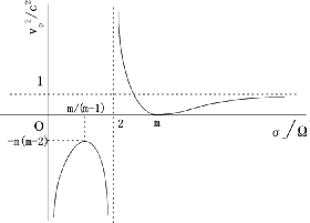
Figure 2: Dispersion relation for negative helicity waves with $m\geq 3$ in a classical limit, $h\rightarrow 1$. The region below horizontal axis corresponds to the evanescent zone. Vertical dotted line denotes the cut-off frequency $\sigma_{-}/\Omega=2$.The resonant absorption frequency is given by $\sigma_{-}/\Omega=2$.

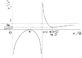
Figure 3: Same as Fig.2 in a relativistic limit, $h\rightarrow 0$. The cut-off frequency is $\sigma_{-}/\Omega=m+2$. The resonant absorption occurs within an evanescent regime at $\sigma_{-}/\Omega=m.$ relation for negative helicity waves with $m\geq 3$ in a classical limit, $h\rightarrow 1$. The region below horizontal axis corresponds to the evanescent zone. Vertical dotted line denotes the cut-off frequency $\sigma_{-}/\Omega=2$. The resonant absorption frequency is given by $\sigma_{-}/\Omega=2$.

3.2 Structure of the Potential Barrier

Figure 4: Spatial structure of the potential barrier for the negative mode as a function of distance. Horizontal dotted line denotes rotation frequency $\sigma_{-}$ of the wave propagating above the potential.

As is obvious from Fig.3, evanescency can not be neglected in large $m$ mode. In this subsection, we turn to the investigation of the spatial structure in the evanescent zone for large $m$. We now introduce a new dependent variable $\Psi_{-}$ defined by $\Psi_{-}\equiv\widetilde{\mu}^{1/2}\xi_{-}$ for the amplitude of the negative mode with $\widetilde{z}\equiv\sqrt{\sigma_{-}}z$. Exploiting some arithmetic algebra, wave equation (21) is now rewritten into a Sturm-Liouville type differential equation

$$\dfrac{d^{2}\Psi_{-}}{d\widetilde{z}^{2}}+\left[\dfrac{1}{4\widetilde{\mu}^{2}}\left(\dfrac{d\widetilde{\mu}}{d\widetilde{z}}\right)^{2}-\dfrac{1}{2\widetilde{\mu}}\dfrac{d^{2}\widetilde{\mu}}{d\widetilde{z}^{2}}+\dfrac{1}{\widetilde{v}^{2}}\left(\widetilde{E}-\widetilde{V}_{m}\right)\right]\Psi_{-}=0,$$ (45)

where

$$\widetilde{E}=\sigma_{-},$$ (46)

$$\widetilde{V}_{m}=\left\{m\left(1-h\right)+2\right\}\Omega.$$ (47)

The first two terms concerning $\widetilde{\mu}$ in square brackets in equation (45) become very small for strong magnetic fields $B_{\text{o}}>10^{14}$ G, since $\widetilde{\mu}$ can be almost regarded as a constant. One can compare equation (45) with the one-dimensional Schrödinger equation for box-type potential in a stationary state. Physical quantities $\widetilde{E}$ and $\widetilde{V}_{m}$ respectively correspond to wave energy and potential in a formal sense. Strictly, potential $\widetilde{V}_{m}$ depends on the wave energy $\widetilde{E}$ through the frequency $\sigma_{-}$. However, $\sigma_{-}$ is here treated as a constant value irrespective of the position, so that the following discussions are valid without loss of generality.

Schematic profile of the effective potential $\widetilde{V}_{m}$ and the wave energy $\widetilde{E}$ are given in Fig.4 as a function of distance $z$. We draw the curve in region (1) somewhat exaggeratedly. The potential varies with the position through the function $h$ and the background rotation $\Omega$. The potential height is determined by the coupled quantity $\left(m+2\right)\Omega$ and its width is given by the size $L$ of the corotating zone. This result means that the large wave number lifts up the potential barrier, only if the background stellar medium rotates. In other words, if surrounding matter is not dragged by the star, say, being in static state $\Omega=0$, then the potential never rises, even though some high azimuthal waves exist.

Whether or not the wave can propagate and transmit out depends on the wave energy, that is, wave frequency $\sigma_{-}$. Our argument deserves to be specially emphasized in two explicit regimes; the evanescent frequency mode $2\Omega<\sigma_{-}<(m+2)\Omega$ and the propagation mode $\sigma_{-}>(m+2)\Omega$.

3.2.1 Evanescent Mode: $2\Omega<\sigma_{-}<(m+2)\Omega$

As is apparent in Fig.4, such low frequency waves excited in the interior cannot help striking the potential barrier. Since refractivity is zero on the critical curve $\sigma_{-}/\Omega=m\left(1-h\right)+2$, outgoing waves with $m\left(1-h\right)+2<\sigma_{-}/\Omega<m+2$ are generally reflected, when they reach the potential wall.

3.2.2 Propagation Mode: $\sigma_{-}>(m+2)\Omega$.

In this case perturbation of the electromagnetic fields can propagate as a wave. The present context in our model is almost concerned with the WKB frequency range. The propagation sometimes exhibits a remarkable property, if certain conditions are satisfied. As long as the wave frequency is much greater than the potential strength $\sigma_{-}\gg(m+2)\Omega$, the potential itself does not have much influence on the wave behavior. However, if the frequency becomes commensurable to the potential height $\sigma_{-}\gtrsim(m+2)\Omega$, the existence of a potential barrier cannot be ignored. Especially if the wavelength is comparable to the potential width, i.e., $k_{-}L\sim 1$, then the waves will interfere with the potential barrier and their behavior will be strongly altered. This inherent property is expected to be more evident near the threshold frequency $\sigma_{-}\sim(m+2)\Omega$. Motivated by this general consideration, we explicitly calculate the transmission rate in the next section. The numerical parameters are adopted to satisfy the above condition, $L\sim 1/k_{-}\sim 10^{6}$ cm and $m=\omega_{\text{max}}/\Omega\sim 10^{6}$. Using these parameters, we will examine how and to what extent the propagation and transmission are affected by the potential barrier.

4 Transmission

4.1 Numerical Calculation

We numerically calculate the transmission rates (42) of the wave propagating from the deep crust, through the corotating plasma envelope, toward the vacuum exterior subject to matching conditions at each boundaries. As already mentioned above, only the negative helicity wave is intriguing for physical interests. Evanescent modes in a low frequency regime $0<\sigma_{-}<\left\{m(1-h)+2\right\}\Omega$ are excluded from this calculation. This constraint on wave frequency thereby guarantees that all waves are capable of propagating in a WKB sense. One can roughly estimate a typical wave frequency $\omega$ measured in the inertial frame by approximating as $\omega\sim\widetilde{v}/q$. Appropriate frequency thus lies in a finite range $10^{3}\lesssim\omega\lesssim 10^{6}$ s^-1.

The objective of this section is to explore the effects of azimuthal wave number $m$ and the size $L$ of the corotating plasma medium on the wave transmission. We here consider two kinds of specific torsional waves whose azimuthal number is; (i) the fundamental, $m=1$ and (ii) much larger than one, $m=\omega_{\text{max}}/\Omega=10^{6}$. In each case, we further consider two apparently different circumstances in the exterior $L=R\sim\lambda_{-}\sim 10^{6}$ cm and in the absence of plasma $L=0$ cm.

Figures 5 and 6 respectively demonstrate the transmission coefficients for the negative helicity waves with two extreme cases (i) $m=1$ and (ii) $m=10^{6}$ as a function of the wave frequency measured in the inertial frame when $B_{\text{o}}=10^{15}$ G, typical for magnetars. In both figures, solid and dotted lines denote the results of $L=10^{6}$ and $L=0$ cm, respectively. The surrounding plasma is here assumed to corotate with the same angular velocity as that of the star, $\Omega=1$ s^-1. In each case, we got the following results.

(i) The Fundamental Wave Number: $m=1$

As seen in Fig.5, the transmission curve in the case of $L=10^{6}$ cm slightly shows a wiggling behavior. This curve intersects that of $L=0$ at $\omega\sim 10^{4}$ s^-1. However, the difference between both cases becomes undistinguishable in the high frequency regime $\omega\gtrsim 10^{5}$ s^-1, since the wave frequency is much higher than the critical one $\left(m+2\right)\Omega=3$ s^-1, which appeared as the potential barrier in section 3. As the wave frequency gets higher, the transmission rate approaches unity asymptotically. Since the overall property does not depend on $L$, the potential barrier due to rotating plasma does not make any significant influence on the wave transmission for small azimuthal number $m\sim 1$.

(ii) Highly Azimuthal Wave Number: $m=10^{6}$

In this high $m$ mode, we can find some suprising results. Figure 6 shows that the transmission rate of $L=10^{6}$ cm is drastically enhanced at some selected frequencies. More importantly, such enhancements occur periodically at specific frequencies. At the top of the first wing $(n=1)$ $\omega_{\text{t}}=2.2\times 10^{3}$ s^-1, the rate reaches the maximum $T_{\text{max}}$=$0.71$, which corresponds to approximately $70$ times larger than that of the first bottom $\omega_{\text{b}}=7.0\times 10^{3}$ s^-1. Comparing with $L=0$ case at the same frequency $\omega_{\text{t}}$, this maximum $T_{\text{max}}$ amounts to $230$ times larger. In this way, plasma effect is important at each top frequency, but unimportant at any bottom frequency. As shown in Fig.6, the transmission coefficient through the plasma layer is exactly equal to that of $L=0$ case at arbitrary wing bottom. In general rotating plasma has an effect in helping the escape of the waves except for the bottom frequencies. This point is different from that of case (i).

Figure 5: Transmission coefficients of the negative helicity wave with the fundamental mode $m=1$as a function of frequency when $B_{\text{o}}=10^{15}$ G and $\Omega=1$ s^-1.Solid and dotted lines denote the results of $L=10^{6}$and $L=0$cm, respectively.

Figure 6: Same as in Figure 5, but for high azimuthal number $m=10^{6}$. In this high $m$ mode transmission rate is highly enhanced at some selected frequencies due to the plasma envelope.

In order to understand the transmission enhancement, we have also numerically computed the integral $\int Td\omega$ in some frequency bands for both $L=10^{6}$ and $L=0$ cm. We obtain some $13$ times enhancement in the narrow band $2\Omega<\omega<\omega_{\text{b}}$ and $1.4$ times in the broad band $2\Omega<\omega<\omega_{\text{max}}$ compared to the results of $L=0$. Such enhancement and periodic variation slowly decrease with increasing wave frequency. This property almost vanishes when the frequency becomes comparable to the critical frequency $\left(m+2\right)\Omega\sim 10^{6}$ s^-1.

Periodic enhancements in our numerical calculations can be interpreted as a consequence of wave interference within the rotating plasma cavity. In the following subsection, we investigate our results more quantitatively in a simplified analytical method.

4.2 Analytical Calculation

Periodic enhancements on the wave transmission in our model can be satisfactorily rationalized by comparing with the wave propagation in homogeneous multi-media. Non-relativistic Alfven resonance itself in the magnetosphere around the earth and the sun have been widely recognized and discussed theoretically and observationally (for recent reviews see Leonovich and Mazur 1997; Waters 2000; Li and Wang 2001). Hollweg (1983) has theoretically studied WKB wave propagation in three homogeneous layers labeled by (1), (2) and (3) separated at $z=0$ and $z=L$ as shown in Fig.7. In his work Alfven waves are simply assumed to have constant wave numbers $k^{(1)}$, $k^{(2)}$ and $k^{(3)}$ in each region. In this homogeneous model, the transmission coefficient $T$ can be analytically calculated by taking boundary conditions at the discontinuities $z=0$ and $z=L$,

$$T=\dfrac{4k^{(3)}}{k^{(1)}}\left[\left\{1+\dfrac{k^{(3)}}{k^{(1)}}\right\}^{2}\cos^{2}(k^{(2)}L)\right.$$

$$\left.+\left\{\dfrac{k^{(3)}}{k^{(2)}}+\dfrac{k^{(2)}}{k^{(1)}}\right\}^{2}\sin^{2}(k^{(2)}L)\right]^{-1}.$$ (48)

Although the physical situation is different from our present work, similar expressions could be found also in our model. This formula (48) implies that the transmission rate has a periodic structure depending on the wave number $k^{(2)}$ and the characteristic scale $L$ of the intermediate layer unless $k^{(2)}L\sim 0$. Extrema of the transmission rate work out to be

$$T_{\text{max}}=\left\{\begin{array}[]{c}\dfrac{4k^{(1)}k^{(3)}}{\left(k^{(1)}+k^{(3)}\right)^{2}}\text{ \ \ at }k^{(2)}L=n\pi,\\ \dfrac{4k^{(1)}k^{(3)}/(k^{(2)})^{2}}{\left(1+k^{(1)}k^{(3)}/(k^{(2)})^{2}\right)^{2}}\text{ \ \ at }k^{(2)}L=\left(2n-1\right)\pi/2,\end{array}\right.$$ (49)

with $n=1,2,\cdots$. Providing that the wave number in each region satisfies the inequalities

$$k^{(1)}\gg k^{(2)}\gg k^{(3)},$$ (50)

$$k^{(2)}L\gtrsim 1,$$ (51)

the coefficient of $\cos^{2}(k^{(2)}L)$ in equation (48) becomes dominant compared to that of $\sin^{2}(k^{(2)}L)$. In this limit, equation (48) can be well approximated by

$$T\approx\dfrac{4k^{(1)}k^{(3)}}{\left(k^{(1)}+k^{(3)}\right)^{2}}\cos^{-2}(k^{(2)}L).$$ (52)

One notices that if $k^{(1)}\sim k^{(2)}\sim k^{(3)}$, the transmission shows neither periodic variations nor enhancements. Consequently, inequalities (50) and (51) give a set of resonant conditions of the wave. Sterling and Hollweg (1984) have subsequently considered a three layer model for solar flare, which is composed of a chromosphere, a spicule and a corona. In that work they have confidently suggested the possibility of Alfvenic resonance on solar spicules and have shown a new aspect of spicules which may account for occasionally twisting motions of magnetic field lines, even when above resonant conditions approximately hold. Conditions (46) and (47) may hold true also in our model except close to the thin regime beneath the stellar surface, whenever large twisted waves with $m\gg 1$ propagate in the rotating background.

We can now quantify the particular frequencies at which the wave resonance occur. By solving the quadratic equation $\left(\sigma_{-}\right)^{2}-\left(m+2\right)\Omega\sigma_{-}-\left(k_{-}^{(2)}\widetilde{v}\right)^{2}=0$, together with the periodic condition $k_{-}^{(2)}L=\left(2n-1\right)\pi$, the eigen frequencies of the negative mode are obtained as

$$\omega_{m,n}=\dfrac{\left(2-m\right)}{2}\Omega+\sqrt{\left(\dfrac{m+2}{2}\Omega\right)^{2}+\left(\dfrac{\left(2n-1\right)c\pi}{2L}\right)^{2}},$$ (53)

with $m,n=1,2,3,\cdots$. This formula shows that the resonant frequencies depend critically on the azimuthal number $m$ and the plasma cavity length $L$. They gently decrease with an increase in $L$ or $m$. Physically, this means that it takes longer time for the wave to go back and forth between the stellar surface and the top of the plasma layer and then this wave interferes with another one propagating from the crust into the cavity. In extremal cases, one finds

$$\lim\limits_{L\rightarrow\infty}\omega_{m,n}=\lim\limits_{m\rightarrow\infty}\omega_{m,n}=2\Omega,$$ (54)

which coincides with the cut-off frequency in the classical limit. At the same time, transmission peaks become blended with neighboring resonance,

$$\lim\limits_{L\rightarrow\infty}\Delta\omega_{m}=\lim\limits_{m\rightarrow\infty}\Delta\omega_{m}=0,$$ (55)

where $\Delta\omega_{m}\equiv\omega_{m,n}-\omega_{m,n-1}$.

For $\Omega=1$ s^-1 and $L=10^{6}$ cm, from equation (53) one can calculate some representative resonant frequencies; the fundamental mode frequency $\omega_{10^{6},1}=8.8\times 10^{3}$ s^-1, the second mode $\omega_{10^{6},2}=7.4\times 10^{4}$ s^-1 and the third $\omega_{10^{6},3}=1.9\times 10^{5}$ s^-1. Our numerical work also gives similar results; $\omega_{10^{6},1}=2.2\times 10^{3}$ s^-1, $\omega_{10^{6},2}=1.9\times 10^{4}$ s^-1 and $\omega_{10^{6},3}=5.2\times 10^{4}$ s^-1, respectively. Our results exhibit slightly positive deviations from the analytical ones. Recall that the wave number $k^{(1)}$ in our magnetar model cannot be regarded as a constant, since the mass density drastically changes in the vicinity of the stellar surface. This discrepancy would be probably attributed to the inhomogeneity in the crust. If a sharp boundary is formed at the stellar surface, such a difference may probably become small. From a comparison with the analytic model, we concluded that the transmission enhancements obtained in our model are thought to be a result of the Alfven resonance on the rotating plasma cavity due to the potential barrier.

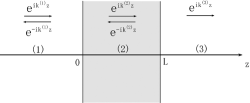
Figure 7: Three homogeneous model separated by two discontinuities at $z=0$ and $z=L$. If periodic boundary condition $k^{(2)}L=n\pi$ $(n=1,2,\cdots)$ holds, intermediate layer acts as a resonant cavity and transmission is highly enhanced.

5 Electromagnetic Field Structure

In the preceding section we have elucidated that the transmission rates of wave are highly enhanced at some selected frequencies owing to the resonance effect in the rotating plasma cavity. Resonance in the plasma portion has another spectacular nature. In this section, it will be shown that resonance has a great impact not only on the transmission rates, but also on the electromagnetic field structure associated with Alfven waves. Most of our applications will once again concern the WKB frequency regime of the negative helicity $\sigma_{-}>\left\{m(1-h)+2\right\}\Omega$. Hereafter we omit the subscript ‘$-$’ for simplicity.

By substituting equation (28) into (11) and (12), we can explicitly have the expressions for electromagnetic field amplitudes in the plasma zone in terms of $k^{(i)}$, normalized by a local magnetic field $B_{\text{o}}$

$$\dfrac{\left|\delta B_{\varpi}\right|^{2}}{B_{\text{o}}^{2}}=\dfrac{\left|\delta B_{\phi}\right|^{2}}{B_{\text{o}}^{2}}=\dfrac{1}{\Omega^{2}\varpi^{2}}\dfrac{\left|c\delta E_{z}\right|^{2}}{B_{\text{o}}^{2}}$$

$$=f_{m}(\varpi)\left|\dfrac{d\xi^{(2)}}{dz}\right|^{2}$$

$$=f_{m}(\varpi)\dfrac{k_{m}^{(1)}}{k^{(3)}}T_{m}\left|A\right|^{2}$$

$$\times\left[(k_{m}^{(2)})^{2}\sin^{2}k_{m}^{(2)}\left(z-L\right)+(k^{(3)})^{2}\cos^{2}k_{m}^{(2)}\left(z-L\right)\right],$$ (56)

and

$$\dfrac{\left|c\delta E_{\varpi}\right|^{2}}{B_{\text{o}}^{2}}=\dfrac{\left|c\delta E_{\phi}\right|^{2}}{B_{\text{o}}^{2}}=f_{m}(\varpi)\sigma_{m}^{2}\left|\xi^{(2)}\right|^{2}$$

$$=f_{m}(\varpi)\left(\sigma_{m}\right)^{2}\dfrac{k_{m}^{(1)}}{(k_{m}^{(2)})^{2}k^{(3)}}\left|A\right|^{2}T_{m}\times$$

$$\left[(k_{m}^{(2)})^{2}\cos^{2}k_{m}^{(2)}(z-L)+(k^{(3)})^{2}\sin^{2}k_{m}^{(2)}(z-L)\right],$$ (57)

where $f_{m}(\varpi)$ is a radial profile given by $f_{m}(\varpi)\equiv(\varpi/\varpi_{\text{pc}})^{2(m-1)}$ $(m=1,2,\cdots)$ and the other notations have the same meaning as the previous ones. The longitudinal component of the perturbed magnetic fields is always zero $\delta B_{z}=0$, because the matter has been assumed to be vertically immobile in the present work. On the contrary, only if the background rotates, the electric fields have a longitudinal component whose structure is essentially identical with that of the magnetic fields. Thereby we only have to investigate the transverse components $(\varpi,\phi)$ of the fields.

For the sake of exploring the dependence of the azimuthal number $m$ on the field structure, we once more restrict our discussions within two kinds of extreme cases: (i) the fundamental mode $m=1$ and (ii) the large azimuthal wave number $m=l\left(\gg 1\right)$. In this limit, formulae (49) and (50) can be well approximated by

$$\dfrac{\left|\delta B_{\varpi}\right|^{2}}{B_{\text{o}}^{2}}=\dfrac{\left|\delta B_{\phi}\right|^{2}}{B_{\text{o}}^{2}}=\dfrac{1}{\Omega^{2}\varpi^{2}}\dfrac{\left|c\delta E_{z}\right|^{2}}{B_{\text{o}}^{2}}$$

$$=\left\{\begin{array}[]{c}f_{m}(\varpi)k_{m}^{(1)}k^{(3)}T_{m}\left|A\right|^{2}\text{ \ \ for }m=1,\\ f_{m}(\varpi)k_{m}^{(1)}k^{(3)}\left(\dfrac{k_{m}^{(2)}}{k^{(3)}}\right)^{2}T_{m}\left|A\right|^{2}\sin^{2}k_{m}^{(2)}\left(z-L\right)\text{ \ }\\ \text{for }m=l,\end{array}\right.$$ (61)

and

$$\dfrac{\left|c\delta E_{\varpi}\right|^{2}}{B_{\text{o}}^{2}} =\dfrac{\left|c\delta E_{\phi}\right|^{2}}{B_{\text{o}}^{2}}$$

$$=\left\{\begin{array}[]{c}f_{m}(\varpi)\sigma_{m}^{2}\dfrac{k_{m}^{(1)}}{k^{(3)}}T_{m}\left|A\right|^{2}\text{ \ \ for }m=1,\\ f_{m}(\varpi)\sigma_{m}^{2}\dfrac{k_{m}^{(1)}}{k^{(3)}}T_{m}\left|A\right|^{2}\cos^{2}k_{m}^{(2)}\left(z-L\right)\text{ }\\ \text{for }m=l.\end{array}\right.$$ (65)

Here we have dropped some small terms coupled to $(k^{(3)})^{2}$, since inequality $k_{m}^{(1)}\gg k_{m}^{(2)}\gg k^{(3)}$ holds for large $m$. Equations (61) and (65) have the implication that the fields are almost constant for small $m$ modes, but are sinusoidally changed with $z$ for large $m$.

In principle, the absolute value of the incident wave amplitude $\left|A\right|$ cannot be determined in our linearized theory. If we are allowed to assume that $f_{m=l}\left(\varpi\right)\left|A\right|_{m=l}^{2}\sim f_{m=1}\left(\varpi\right)\left|A\right|_{m=1}^{2}$, then the ratios of electromagnetic field amlitude with $m=l$ to those with $m=1$ are approximately given by

$$\dfrac{\left|\delta B_{i}\right|_{m=l}^{2}}{\left|\delta B_{i}\right|_{m=1}^{2}}\approx\left(1+\dfrac{l\Omega}{\omega}\right)^{2}\left(1-\dfrac{2\Omega}{\omega}\right)\dfrac{T_{m=l}}{T_{m=1}}\sin^{2}k_{m}^{(2)}\left(z-L\right),$$ (66)

and

$$\dfrac{\left|\delta E_{i}\right|_{m=l}^{2}}{\left|\delta E_{i}\right|_{m=1}^{2}}\approx\left(1+\dfrac{l\Omega}{\omega}\right)^{3}\left(1+\dfrac{\Omega}{\omega}\right)^{-2}\dfrac{T_{m=l}}{T_{m=1}}\cos^{2}k_{m}^{(2)}\left(z-L\right),$$ (67)

with $i=\varpi,\phi$. These quantities are much larger than unity because of the extra factor $\left(1+l\Omega/\omega\right)$ except for some special locations $z=n\pi/k_{m}^{(2)}$ and $z=(2n-1)\pi/2k_{m}^{(2)}$ $(m,n=1,2,\cdots),$ which correspond to the nodes of the standing Alfven wave.

Figure 8: Spatial structure of perturbed magnetic field with $m=1$ in the rotating plasma region normalized by that in the absence of plasma at some resonant frequencies in the first wing. The solid and the dotted lines denote the result at the top of wing $\omega_{\text{t}}=2.2\times 10^{3}$ s^-1 and at the bottom $\omega_{\text{b}}=7.0\times 10^{3}$ s^-1, respectively.

Figure 9: Same as in Fig.8 for $m=10^{6}$. Field amplitudes are drastically and periodically enhanced for large $m$. This enlargement is attributed to the resonance transmission and the conservation of energy flux as a multiplier effect.

We will now examine the effect of the resonance in the rotating plasma cavity, whose thickness is given by $L\sim R=10^{6}$ cm, on the spatial structure of the perturbed electromagnetic fields. Let us designate by $\alpha$ the amplitude of the perturbed magnetic field within the plasma normalized by that in the absence of the plasma

$$\alpha(z) \equiv \dfrac{\left|\delta B_{i}\right|_{L=R}^{2}}{\left|\delta B_{i}\right|_{L=0}^{2}}$$ (68)

$$\approx \dfrac{T_{L=R}}{T_{L=0}}\dfrac{c^{2}}{\omega^{2}}\times$$

$$\left[\left\{(k_{m}^{(2)})^{2}-\dfrac{\omega^{2}}{c^{2}}\right\}\sin^{2}k_{m}^{(2)}\left(z-L\right)+\dfrac{\omega^{2}}{c^{2}}\right].\text{ \ \ }$$

The first term in square brackets is related to the deviation due to high torsional modes in the rotating background from the dispersion relation in a vacuum. The ratio $\alpha$ is plotted against the height from the stellar surface for (i) $m=1$ in Fig.8 and (ii) $m=10^{6}$ in Fig.9, respectively. Solid lines denote the numerical results at the top of the wing $\omega_{\text{t}}=2.2\times 10^{3}$ s^-1, while dotted lines denote the bottom $\omega_{\text{b}}=7.0\times 10^{3}$ s ^-1. The transmission rates at resonant frequencies obtained in section 3 are appropriately used in this calculation.

(i) The Fundamental Wave Number: $m=1$

As shown in Fig.8, in the case of $m=1,$ the wave amplitude keeps one order of magnitude in the plasma. This result agrees well with the fact that the dispersion relation for small $m\sim 1$ is almost equal to that of the electromagnetic fields in pure vacuum, $(k_{m}^{(2)})^{2}\sim\omega^{2}/c^{2}$. The background rotation therefore does not affect this small $m$ modes.

(ii) Highly Azimuthal Wave Number: $m=10^{6}$

Some significant differences can be found in this high mode. The perturbed magnetic field strength $\alpha$ for $m=10^{6}$ at the resonant frequency $\omega_{\text{t}}$ is drastically amplified up to $\alpha\sim 10^{5}$ at $z\lesssim 10^{5}$ cm. Then the field strength $\alpha$ is fallen down to $\alpha=T_{L=R}/T_{L=0}\sim 230$ at the top of the plasma layer, in which the first node of the standing Alfven wave is formed. Even at the bottom frequency $\omega_{\text{b}}$ the strength $\alpha$ has about $10^{2}$ at $z\simeq 5\times 10^{5}$ cm.

In the same way, the normalized amplitude of the perturbed electric field is expressed by

$$\beta(z) \equiv \dfrac{\left|\delta E_{i}\right|_{L=R}^{2}}{\left|\delta E_{i}\right|_{L=0}^{2}}$$ (69)

$$= \dfrac{T_{L=R}}{T_{L=0}}\left(1+\dfrac{m\Omega}{\omega}\right)^{2}\dfrac{1}{(k_{m}^{(2)})^{2}}\times$$

$$\left[\left\{(k_{m}^{(2)})^{2}-\dfrac{\omega^{2}}{c^{2}}\right\}\cos^{2}k_{m}^{(2)}\left(z-L\right)+\dfrac{\omega^{2}}{c^{2}}\right],\$$

which is plotted in Figs.10 and 11. When $m=10^{6}$, the field amplitude $\beta$ of $\omega_{\text{t}}$ has almost the same magnitude $10^{5}$ as $\alpha$ near the stellar surface $z\lesssim 10^{4}$ cm. But near the top of the plasma $z\sim 10^{6}$ cm, in contrast to $\alpha$, $\beta$ has a maximum $5\times 10^{7}$ which corresponds to the loops of the standing wave. Approximately, $\beta$ is much greater than $\alpha$ because of the extra term $\left(1+m\Omega/\omega\right)^{2}\sim 10^{6}$ in equation (69).

Such a field amplification can also be explained by considering a conservation of energy flux $F\sim\widetilde{\rho}v\omega\left|\xi\right|^{2}$. The phase velocity $v$ of the mode $m\gg 1$ in the plasma atmosphere is much smaller than that in the vacuum, as is confirmed in equations (43) and (44). Assuming the same value $\left|\xi\right|$ at the stellar surface, which is irrelevant to $L$, the amplitude $\left|\xi\right|(\varpropto v^{-1/2})$ is enhanced in the rotating plasma region so as to compensate for the slowing down of the wave propagation.

Figure 10: Perturbed electric fields with $m=1$ in the rotating plasma at resonant frequencies in the first wing. Solid line and dotted line respectively correspond to $\omega_{\text{t}}=2.2\times 10^{3}$ s^-1 and $\omega_{\text{b}}=7.0\times 10^{3}$ s^-1.

Figure 11: Same as in Fig.10 for $m=10^{6}.$

6 Summary and Discussion

We have studied the propagation and transmission of torsional Alfven waves along the rotation axis on magnetars by using three-layered cylindrical model. If the intermediate plasma layer rotates with angular velocity $\Omega$, the propagation property for largely twisted waves with $m>\omega/\Omega$ is drastically modified. This middle zone can be regarded as a kind of a potential barrier, whose height is explicitly specified by $(m+2)\Omega$. Waves having an angular velocity of $2\Omega$ originates from Coriolis force in the classical limit, while an additional quantity $m\Omega$ comes from the relativistic effect. This therefore means that the potential is lifted up higher in the large $m$ modes on the rotating background. It should be emphasized that this new finding is purely attributed to having incorporated the displacement current into the model.

We have numerically computed the transmission rates of the torsional waves with large value $m\gg 1$ driven in the crust, through the corotating plasma with a finite size $L\sim R$, into the exterior. We found that the transmissions are strongly enhanced for large $m\approx\omega/\Omega$ at selected wave frequencies satisfied with a periodic condition $kL\simeq\left(2n-1\right)\pi/2$ $(n=1,2,\cdots)$. Such a transmission enhancement arises because the rotating plasma forms a resonant cavity which traps the wave energy by virtue of the strong reflections occuring at the transition region at the bottom and at the top of the plasma layer. Efficient transmissions due to resonance is also compatible with the fact that the reflection of waves at the stellar surface can almost completely be extinguished. Magnetospheric waveguide or resonance cavity can thus actually generate a set of coherent eigenmodes for high $m$. Resonance may be a signature of fundamental processes by which high order torsional oscillations of waves, if there exists, can transfer much more energy out of the magnetars especially in the low frequency regime.

It has been well-known in quantum mechanics that when the potential width is comparable to (or integer times) de Broglie wavelength of electrons $L\sim n\hbar/m_{\text{e}}v$, incident wave flux is bounded by finely tuning a phase relation with inversely propagating waves (e.g., Schiff 1949). Then resonance is excited in the potential zone and the wave flux spends much of its time in the resonance cavity. Similar resonance may occur also in our macroscopic model, if the characteristic scale of the evanescent zone is comparable to the wavelength of the Alfven wave.

We have investigated the spatial structure of the perturbed electromagnetic fields propagating in the rotating plasma, when standing Alfven waves are formed. Resonance in the plasma cavity for high $m$ modes has another spectacular aspect. At some points magnetic fields of the Alfven waves are drastically amplified even up to a few $10^{5}$ times as large as those in the absence of plasma or in the static exterior. This amplification can be straightforwardly explained by both the transmission enhancement due to resonance and the conservation of WKB energy flux.

In this way, once the Alfven waves are resonantly excited and transmissions are greatly enhanced, a substantial part of the wave energy will probably be transferred into the ambient charged particles such as electrons or positrons confined within the fire balls associated with the bursts on magnetars. The charged particles entwined around magnetic field lines will then be violently swayed. These disturbances may eventually produce high energy $\gamma$-ray or X-ray emissions from the magnetars. More importantly, if magnetic field lines at some altitudes are strongly distorted from equilibrium state by resonance and plasma fluid contracts into the surface, the field lines with antiparallel components will approach each other. Such geometry of field lines will give rise to possible magnetic reconnection type events as Thompson and Duncan (2000) have suggested.

The behavior of resonant MHD waves within the corona or spicules erupted from the solar surface have been studied so far. In fact, field line resonance has been found to occur on magnetic shells in the magnetosphere of the earth. But their physical treatment is inevitably restricted to the very weak magnetic fields. Resonant property found in our magnetar model is very similar to that in solar astrophysics or planetary physics. We can expect that the same mechanism works also on the relativistic Alfven waves even in a different environment, that is, in an extreme circumstance accompanied by very strong magnetic fields such as the magnetars.

As a final remark, we shall address on the angular velocity $\Omega$ of the star and the azimuthal wave number $m$. In our model, the rotating background is throughout assumed to have a slow angular velocity $\Omega=1$ s^-1, which is actually observed in SGRs and AXPs. We concentrate our treatment on the torsional waves with a specific value $m=10^{6}$ as a possible limit of high $m$. As shown in our work, the striking behavior of the resonance necessarily requires high order torsional modes, $m>\omega/(1$ s${}^{-1})\simeq 10^{3}$-$10^{6}$. It is not clear whether or not such modes with high wave number $m$ realistically exist on the magnetars. However, one should keep it in mind that the local dispersion relation of the Alfven waves are almost determined by the coupled quantity $m\Omega$ except for the high frequency regime. This means that the physical behavior of the wave with high $m=10^{3}$-$10^{6}$ on the slowly rotating background$\ \Omega=1$ s^-1 is essentially equivalent to that of small $m=1$-$10^{3}$ and fast rotation $\Omega=10^{3}$ s^-1. Neutron stars are often expected to have been a rapid rotator with $\Omega\sim 10^{3}$ s^-1 at a star-born period. Our results would thus become much more effective especially on young magnetars.

Appendix

The physical effects of $\gamma$ can be clarified by taking some explicit limits. Specifically if one ignores the substantial thickness of the plasma layer $L\rightarrow 0$, then the wave number of region (2) should be replaced with that of region (3), $k_{\pm}^{(2)}\rightarrow k^{(3)}$. This yields that $\varkappa_{+}\rightarrow 2k^{(3)},\varkappa_{-}\rightarrow 0$ and $\gamma\rightarrow 1$. In this limit, the boundary condition reduces to $d/dz[\ln\xi_{\pm}^{(2)}]=ik^{(3)}$, which clearly corresponds to the simple case that the exterior of the star is filled with pure vacuum or static plasma gas. While, if one imagines the very huge plasma gas corotating in the exterior and takes the limit formally $L\rightarrow\infty$, then the wave number of region (3) should be equal to that of region (2), $k^{(3)}\rightarrow k_{\pm}^{(2)}$. We thus have that $\varkappa_{+}\rightarrow 2k_{\pm}^{(2)},\varkappa_{-}\rightarrow 0$ and $\gamma\rightarrow 1$, which yield the boundary condition $d/dz[\ln\xi_{\pm}^{(2)}]=ik_{\pm}^{(2)}$.

One can draw some important facts from the boundary condition (35). Especially when the wave number satisfies the periodic condition $\varkappa_{\pm}L=n\pi$ $(n=1,2,\cdots)$, this yields $\gamma=k^{(3)}/k_{\pm}^{(2)}$ and thereby the boundary condition for pure vacuum is recovered $d/dz[\ln\xi_{\pm}^{(2)}]=ik^{(3)}$. The background rotation has no influence only on the Alfven waves satisfied with this condition. Whereas, when the wave number satisfies the another periodic condition $\varkappa_{\pm}L=(2n-1)\pi/2$ $(n=1,2,\cdots)$, one obtains $\gamma=k_{\pm}^{(2)}/k^{(3)}$ and thus the boundary condition works out to be $d/dz[\ln\xi_{\pm}^{(2)}]=ik^{(3)}(k_{\pm}^{(2)}/k^{(3)})^{2}\gg ik^{(3)}$. The RHS of this expression turns out that the waves satisfied with this condition are highly transmitted, as far as $k_{\pm}^{(1)}$ does not change much over one wavelength, say the validity of WKB approximation $\left(1/k_{\pm}^{(1)}\right)\left|dk_{\pm}^{(1)}/dz\right|\ll k_{\pm}^{(1)}$ holds. This peculiar result means that the internal shear modes can be coupled onto the high frequency Alfven modes at the stellar surface, which drastically enhances their transmission rate at certain wave numbers or frequencies.

This work is supported in part by Grants-in-Aid for Scientific Research (14047215, 16029207, and 16540256) from the Japanese Ministry of Education, Culture, Sports, Science, and Technology.

References

- (1) Blaes, O., Blandford, R., Goldreich, P., & Madau, P. 1989, ApJ, 343, 839
- (2) Cheng, B., Epstein, R. I., Guyer, R. A., & Young, C. 1996, Nature, 382, 518
- (3) Feroci, M., Duncan, R. C., & Thompson, C. 2001, ApJ, 549, 1021
- (4) Gogus, E., et al. 1999, ApJ, 526, L93
- (5) Gogus, E., et al. 2000, ApJ, 532, L121
- (6) Hollweg, J.V. 1983, Solar Phys, 91, 269
- (7) Huang, Y. F., Dai, Z. G., & Lu, T. 1998, Chinese Phys. Lett., 15, 775
- (8) Hurley, K., et al. 1999a, ApJ, 510, L111
- (9) Hurley, K., et al. 1999b, Nature, 397, 41
- (10) Hurley, K., et al. 2000, ApJ, 528, L21
- (11) Hurley, K., et al. 2005, Nature, 434, 1098
- (12) Jackson, J. D. 1975, Classical Electrodynamics (New York: Wiely), chap. 8.
- (13) Kojima, Y., & Okita, T. 2004, ApJ, 614, 922
- (14) Kouvelioutou, C., et al. 1993 Nature, 362, 728
- (15) Kouvelioutou, C., et al. 1998, Nature, 393, 235
- (16) Leonovich, A.S, & Mazur, V.A. 1997, Ann Geophys, 16, 900
- (17) Li B., & Wang, S. 2001, A&A, 25, 446
- (18) Mazets, E. P., et al. 1979, Nature, 282, 587
- (19) Mazets, E. P., Golenetskii, S. V., & Gur’yan, Yu. A. 1979, Soviet Atron. Lett., 5(6), 343
- (20) Mazets, E. P., et al. 1999, Astro. Lett., 25(10), 635
- (21) Mereghetti, S., & Stella, L. 1995, ApJ, 442, L17
- (22) Mereghetii, S. 2000, The Neutron Star-Black Hole Connection, ed. Kouveliotou, C., Ventura, J., & van den Heuvel, E. P. J. (Dordrecht: Reidel), in press
- (23) Mereghetti, S., Chiarlone, L., Israel, G. L., & Stella, L. 2002, Proc. 270th WE-Heraeus Seminar on Neutron Stars, Pulsars, and Supernova Remnants, ed. Becker, W., Lesch, H., & Trümper, J., (MPE Rep. 278; Garching: MPI), 29
- (24) Mereghetti, S., et al. 2005, ApJ, 624, L105
- (25) Pacini, F., & Ruderman, M. 1974, Nature, 251, 399
- (26) Palmer, D. M., et al. 2005, Nature, 434, 1107
- (27) Rea, N., et al. 2005, ApJ, 627, L133
- (28) Shiff, L. I., Quantum Mechanics (3rd ed.), McGraw-Hill, 1968
- (29) Sterling, A. C., & Hollweg, J. V. 1984, ApJ, 285, 843
- (30) Sterling, A. C. 1998, ApJ, 508, 916
- (31) Thompson, C., Duncan, R. C., Woods, P. M., Kouveliotou, C., Finger, M. H., & van Paradijs, J. 2000, ApJ, 543, 340
- (32) Thompson, C., & Duncan, R. C. 2001, ApJ, 561, 980
- (33) Waters, C.L., 2000, Adv, Space Res., Vol.25, No. 7/8, 1541
- (34) Wolfgang, B., & Rudolf, A. T. 1996, Basic Space Plasma Physics (Imperial College Press)