The Impact of Temperature Fluctuations on the Ly$\alpha$ Forest Power Spectrum

Abstract

We explore the impact of spatial fluctuations in the intergalactic medium temperature on the Ly$\alpha$ forest flux power spectrum near $z\sim 3$. We develop a semianalytic model to examine temperature fluctuations resulting from inhomogeneous H I and incomplete He II reionizations. Detection of these fluctuations might provide insight into the reionization histories of hydrogen and helium. Furthermore, these fluctuations, neglected in previous analyses, could bias constraints on cosmological parameters from the Ly$\alpha$ forest. We find that the temperature fluctuations resulting from inhomogeneous H I reionization are likely to be very small, with an rms amplitude of $\lesssim 5\%$, $\sigma_{T_{0}}/\langle T_{0}\rangle\lesssim 0.05$. More important are the temperature fluctuations that arise from incomplete He II reionization, which might plausibly be as large as $50\%$, $\sigma_{T_{0}}/\langle T_{0}\rangle\sim 0.5$. In practice, however, these temperature fluctuations have only a small effect on flux power spectrum predictions. The smallness of the effect is possibly due to density fluctuations dominating over temperature fluctuations on the scales probed by current measurements. On the largest scales currently probed, $k\sim 0.001$ s km^-1 ($\sim$0.1 $h$ Mpc^-1), the effect on the flux power spectrum may be as large as $\sim 10\%$ in extreme models. The effect is larger on small scales, up to $\sim 20\%$ at $k=0.1$ s km^-1, due to thermal broadening. Our results suggest that the omission of temperature fluctuations effects from previous analyses does not significantly bias constraints on cosmological parameters.

1. Introduction

In the current theoretical picture of the Ly$\alpha$ forest, most of the structure in the forest is a product of gravitational instability. The absorbing gas is assumed to be in photoionization equilibrium with a spatially homogeneous radiation field. On large scales the hydrogen gas distribution follows the dark matter distribution, and on small scales it is Jeans pressure-smoothed (see e.g., Cen et al., 1994; Zhang et al., 1995; Hernquist et al., 1996; Miralda-Escude et al., 1996; Muecket et al., 1996; Bi & Davidsen, 1997; Bond & Wadsley, 1997; Hui et al., 1997; Croft et al., 1998; Bryan et al., 1999; Davé et al., 1999; Theuns et al., 1999; Nusser & Haehnelt, 1999). This gravitational instability model of the forest, motivated by numerical simulations, seems to agree well with observations (e.g. Croft et al., 2002; McDonald et al., 2005b; Tytler et al., 2004; Viel et al., 2004; Lidz et al., 2006).

In this model, each Ly$\alpha$ forest spectrum provides a one-dimensional map of the density field in the intergalactic medium (IGM). The Ly$\alpha$ forest can thus be used to constrain the amplitude and slope of the linear matter power spectrum at $z\sim 3$ on scales of $k\sim 0.1-5\,h\,{\rm Mpc^{-1}}$ (see e.g., Croft et al., 1998; McDonald et al., 2000; Zaldarriaga et al., 2001a; Croft et al., 2002; Zaldarriaga et al., 2003). When combined with measurements from Cosmic Microwave Background (CMB) experiments and galaxy surveys, the Ly$\alpha$ forest provides important constraints on cosmological parameters (e.g. Seljak et al., 2005; Viel et al., 2005b). Recently, very tight constraints on cosmological parameters were derived using measurements of the Ly$\alpha$ forest flux power spectrum from the Sloan Digital Sky Survey (SDSS) (McDonald et al., 2006, 2005b; Seljak et al., 2005). The data samples used in the SDSS flux power spectrum measurements are almost two orders of magnitude larger than those used in previous measurements. The increase in statistical precision sets a high bar for the required control over systematic effects in theoretical predictions. The key issues are now to devise consistency checks for the gravitational instability model of the Ly$\alpha$ forest, to quantify the accuracy of our theoretical modeling, and to improve the modeling when possible. These steps are essential in order to estimate the systematic-error budget in the modeling, and to utilize the full statistical power of the SDSS measurements.

Toward this end, we point out that previous models of the Ly$\alpha$ forest adopt an over-simplified description of the IGM reionization history and the resulting thermal evolution. Specifically, previous models assume that reionization is sudden and uniform, so that in effect each gas element in the IGM experiences the same reionization history. In reality, reionization is likely to be an extended and inhomogeneous process (Sokasian et al., 2003, 2004; Barkana & Loeb, 2004; Furlanetto et al., 2004; Babich & Loeb, 2006), with some gas elements reionizing earlier than others, and hence cooling to lower temperatures by $z\sim 3$ (e.g. Hui & Haiman, 2003). Furthermore, He II may be reionized by bright quasars, and the process may be incomplete near $z\sim 3$. In this case, the IGM at $z\sim 3$ resembles a two-phase medium. The first phase consists of regions that have already been engulfed by the He III ionization fronts that are expanding around bright quasars. These regions, recently photo-heated by a hard quasar spectrum, may have temperatures in excess of $\sim 3\times 10^{4}\mbox{ K}$ (Abel & Haehnelt, 1999). The second phase consists of regions where He II has yet to reionize, but have H I/He I reionized at early times. In this phase, gas elements with density near the cosmic mean will be significantly cooler, with temperatures of $\sim 1\times 10^{4}\mbox{ K}$. These temperature fluctuations should be imprinted in the Ly$\alpha$ forest since the widths of Ly$\alpha$ absorption lines, as well as the hydrogen recombination coefficient, and hence the optical depth to Ly$\alpha$ absorption, depend on temperature.

The goal of this paper is to estimate the amplitude and spatial scale of the temperature fluctuations resulting from H I and He II reionization, and to examine their impact on the flux power spectrum. Temperature fluctuations are particularly interesting because if they significantly impact the flux power spectrum, then their detection would likely provide insights into the reionization histories of hydrogen and helium. Furthermore, we reiterate that it is important to check whether omitting temperature fluctuations in the analyses will significantly bias the determination of cosmological parameters from the Ly$\alpha$ forest.

The outline of this paper is as follows. We begin with a brief overview of the theoretical model describing the Ly$\alpha$ forest in § 2. We then estimate the amplitude of temperature fluctuations expected from inhomogeneous H I reionization in § 3. In § 4 we estimate the amplitude and scale of temperature fluctuations for a range of models describing He II reionization by bright quasars, using the observed quasar luminosity function as input. In § 5, we examine the impact of these fluctuations on the flux power spectrum. We conclude in § 6 and discuss possible future research directions.

2. Modeling the Ly$\alpha$ Forest

In this section, we briefly review the standard theoretical model of the Ly$\alpha$ forest in order to introduce notation, and highlight the approximations that we subsequently test in this paper. For more details, the reader can refer to e.g., Hui et al. (1997).

The gas responsible for the absorption in the Ly$\alpha$ forest is thought to be in photoionization equilibrium with a radiation background produced by star-forming galaxies and/or quasars. In this case, the abundance of neutral hydrogen scales like $n_{\rm HI}\propto\alpha(T)\Delta^{2}/\Gamma$. Here, $\alpha(T)\propto T^{-0.7}$ is the temperature dependent hydrogen recombination coefficient, $\Delta$ is the baryon density in units of the cosmic mean, and $\Gamma$ is the hydrogen photoionization rate. The optical depth to Ly$\alpha$ absorption is proportional to the neutral hydrogen abundance (besides thermal broadening and peculiar velocities), which implies a simple power-law relationship between the Ly$\alpha$ optical depth and the gas density. Therefore, if the gas temperature and $\Gamma$ are known or can be modeled, then there exists a direct connection between the Ly$\alpha$ absorption and the underlying density fluctuations.

Indeed, the physics that sets the temperature of the absorbing gas is expected to be relatively simple. The gas temperature is determined largely by the competition between photoionization heating and adiabatic cooling (Miralda-Escude & Rees, 1994; Hui & Gnedin, 1997). In this case, the temperature of the low density gas, where shock-heating should be unimportant, is expected to be tightly correlated with its density (Hui & Gnedin, 1997). In fact, these authors show that the gas temperature should be a power-law in the gas density: $T=T_{0}\Delta^{\gamma-1}$. The numerical values of the power law index, $\gamma$, and the temperature at mean density, $T_{0}$, depend on when the gas was reionized and the nature of the ionizing sources (e.g. Hui & Gnedin, 1997; Abel & Haehnelt, 1999; Sokasian et al., 2002; Theuns et al., 2002a; Hui & Haiman, 2003).

The standard assumption is that $\Gamma$, $T_{0}$ and $\gamma$ are all spatially uniform, i.e. they have a single value throughout the entire IGM. To the extent that this is true, the neutral hydrogen density, and hence the Ly$\alpha$ optical depth, scales as $\tau=A_{\tau}\Delta^{2-0.7(\gamma-1)}$, where the proportionality constant $A_{\tau}$ is independent of spatial position. In this simple case, fluctuations in the Ly$\alpha$ forest absorption directly traces the underlying density fluctuations. Several authors have investigated the possible ‘contamination’ from spatial fluctuations in the hydrogen photoionization rate, $\Gamma$, finding that these fluctuations should be quite small near $z\sim 3$ (Croft et al., 1999; Meiksin & White, 2004; Croft, 2004; McDonald et al., 2005a). Little attention, however, has been given to the assumption that $T_{0}$ and $\gamma$ are also spatially uniform.

In the case where $T_{0}$ and $\gamma$ fluctuate spatially, the relation for the Ly$\alpha$ optical depth generalizes to:

$$\tau=A_{\tau}\Delta^{2-0.7(\gamma-1)}(1+\delta_{T_{0}})^{-0.7}.$$ (1)

The new ingredient in this equation is the term $1+\delta_{T_{0}}=T_{0}/\langle T_{0}\rangle$ which represents spatial fluctuations in the temperature of the gas at the cosmic mean density. Furthermore, we consider spatial fluctuations in $\gamma$, i.e. $\gamma$ in this equation now depends on position. Additionally, fluctuations in the IGM temperature lead to spatial variations in the thermal broadening kernel, which will affect the Ly$\alpha$ forest on small scales.

The flux transmitted through the Ly$\alpha$ forest, after taking into account peculiar velocities and thermal broadening, is given by $F=e^{-\tau}$. Fluctuations in the transmission are given by $\delta_{F}=(F-\langle F\rangle)/\langle F\rangle$, and the power spectrum of $\delta_{F}$ is the flux power spectrum, which we denote by $P_{F}(k)$. Our goal then is to explore the impact of the temperature fluctuations encoded in Eq. 1, and in the thermal broadening kernel, on the flux power spectrum $P_{F}(k)$.

3. Temperature Fluctuations from Inhomogeneous H I Reionization

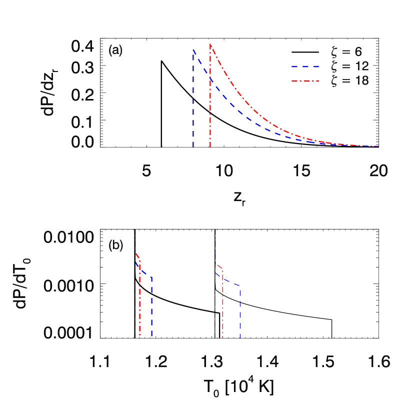
Figure 1.— Panel (a): H I reionization redshift distribution for $\zeta$ = 6, 12, and 18. Panel (b): Temperature distribution at $z=3$ for the same reionization models in (a). The thick (thin) curves are calculated using $T_{r}=2.5\times 10^{4}$ K ($3\times 10^{4}$ K).

We begin by considering the amplitude of temperature fluctuations resulting from H I reionization, which recent theoretical work has emphasized to be likely inhomogeneous and extended (Sokasian et al., 2003; Barkana & Loeb, 2004; Furlanetto et al., 2004; Babich & Loeb, 2006). We use the model of Furlanetto et al. (2004) to describe the duration of extended H I reionization, and scaling relations from Hui & Gnedin (1997) to estimate the amplitude of the resulting temperature fluctuations. Throughout this paper, we will work generally within the context of a model in which H I/He I are reionized at high redshift by star-forming galaxies, while He II is reionized close to $z\sim 3$ by quasars. This is not the only possibility (see Lidz et al. 2005, in prep., for a discussion), and so it is useful for us to explicitly separate out the temperature fluctuations that arise from H I reionization and those that arise from He II reionization. The case that H I and He II are both reionized at high redshift will then be similar to our H I calculation: the only difference being that the temperature at reionization would likely be higher, and the duration of the reionization process might be different.

The Furlanetto et al. (2004) model describes the growth and overlap of H II regions during reionization. The basic picture in this model is that large scale overdense regions contain more ionizing sources, and are reionized earlier, than underdense regions. The model assumes that a galaxy of mass $m_{\rm gal}$ can ionize a mass corresponding to $\zeta m_{\rm gal}$, where $\zeta$ is an unknown parameter describing how efficiently a galaxy can ionize surrounding gas (see Furlanetto & Oh 2005 and Furlanetto et al. 2006 for extensions to this model). A region is considered ionized when the the fraction of mass in halos more massive than some minimum mass, $m_{\rm min}$, exceeds a threshold set by the ionization efficiency of the sources: $f_{\rm coll}>\zeta^{-1}$. Here, $f_{\rm coll}$ denotes the fraction of mass in the region which has collapsed into halos of mass larger than $m_{\rm min}$. In this case, the size distribution of H II regions can be calculated in a similar manner to the halo mass function in the excursion set formalism (e.g., Bond et al., 1991; Lacey & Cole, 1993).

The Furlanetto et al. (2004) model predicts, given $\zeta$, the filling factor of ionized regions. It is given by

$$Q=\zeta\bar{f}_{\rm coll}$$ (2)

where $\bar{f}_{\rm coll}$ is the global collapse fraction (different from $f_{\rm coll}$, the collapse fraction of a region with a given overdensity). In the extended Press-Schechter theory, the global collapse fraction is given by (Bond et al., 1991; Lacey & Cole, 1993):

$$\bar{f}_{\rm coll}={\rm erfc}\left[\frac{\delta_{\rm c}(z)}{\sqrt{2\sigma_{\rm min}^{2}(z)}}\right],$$ (3)

where $\delta_{\rm c}(z)$ is the critical density for collapse and $\sigma_{\rm min}^{2}(z)$ is the density variance on the scale of $m_{\rm min}$, the minimum mass of an ionizing source. We take the minimum mass to be the mass corresponding to a virial temperature of $10^{4}\mbox{ K}$, where atomic hydrogen line cooling is efficient.

The probability distribution of reionization redshift is related to the filling factor $Q$ by

$$\frac{dP}{dz_{r}}=\left.-\frac{dQ}{dz}\right|_{z=z_{r}}.$$ (4)

In Fig. 1a, we plot $dP/dz_{r}$ for $\zeta$ = 6, 12, and 18. The curves terminate when $Q=1$, corresponding to the end of reionization. The figure clearly illustrates that H I reionization should be quite extended, with the whole process taking place over a $\Delta z$ of several. The end, and somewhat the duration, of reionization naturally depends on how efficiently the sources produce ionizing photons, which is quite uncertain. We therefore consider $\zeta$ = 6, 12, and 18, in which case the end of reionization occurs at $z=$ 6, 8, and 9 respectively. For our purposes, these choices of $\zeta$ bracket the interesting range of possibilities. It is uninteresting to consider sources that are much less efficient, because we know the IGM is highly ionized below $z\sim 6$ (e.g. Fan et al., 2002). On the other hand, more efficient sources would lead to a very early end to reionization, in which case the temperature at lower redshifts is completely insensitive to when precisely the gas was reionized owing to efficient Compton cooling (Hui & Haiman, 2003).

In order to investigate the temperature fluctuations that result from extended H I reionization, we rely on analytic approximations by Hui & Gnedin (1997) to describe the thermal history of the IGM. These analytic approximations derive from the fact that the temperature of the low density gas is primarily determined by photoionization heating and adiabatic cooling. Under these simple physical conditions, Hui & Gnedin (1997) give formulae for the evolution of $T_{0}$ and $\gamma$ (see their Eq. 19 and 22). The input to these formulae is simply the temperature, $T_{r}$, that a gas element reaches when it is reionized at redshift $z_{r}$. Given $T_{r}$, these formulae give the values of $T_{0}$ and $\gamma$ at lower redshifts, $z<z_{r}$.

The temperature at reionization, $T_{r}$, is quite uncertain. It is determined both by the intrinsic spectrum of the ionizing sources, and the hardening of the spectrum owing to absorption in the IGM (Abel & Haehnelt, 1999). Scatter in the intrinsic and re-processed spectra will likely give rise to a distribution of $T_{r}$. It is also unclear that gas elements reionized at different times, albeit by sources with the same intrinsic spectrum, will reach the same temperature following reionization. We currently ignore these subtleties in our model, and assume that all gas elements will reionize to the same $T_{r}$. The value $T_{r}=2.5\times 10^{4}\mbox{ K}$ is reasonable assuming that galaxies are the ionizing sources (Hui & Gnedin, 1997). We also investigate the effects of using a more extreme $T_{r}=3\times 10^{4}\mbox{ K}$. Note that because of the high abundance of galaxies, each gas element will likely see the combined radiation from numerous sources during reionization. This will tend to average out the scatter in the intrinsic and re-processed spectra, so a uniform $T_{r}$ is probably a good approximation. The same may not be true if quasars are the ionizing sources, since quasars are sparse and each gas element will only see the radiation from one, or a few, nearby sources.

With $z$ and $T_{r}$ fixed, $T_{0}$ is a function of $z_{r}$ only and we can find the distribution of $T_{0}$ with the simple transformation:

$$\frac{dP}{dT_{0}}=\frac{dP}{dz_{r}}\left|\frac{dT_{0}}{dz_{r}}\right|^{-1}.$$ (5)

The temperature distribution is plotted in Fig. 1b. The cutoff in the distribution at high $T_{0}$ occurs because there is a definite end to reionization in our model, after which the probability of reionization is formally zero. The upper temperature limit to the distribution is therefore set by the $T_{0}$ of the most recently reionized gas elements. There is a sharp rise in the temperature distribution at low $T_{0}$, because gas elements reionized above $z\sim 10$ will have reached almost the same temperature at low redshift, owing to efficient Compton cooling at high redshift (Hui & Gnedin, 1997).

The temperature distribution at $z=3$ spans a very narrow range in $T_{0}$, generally less than a few hundred degrees Kelvin, in all the models we consider. This is because the interplay between photoionization heating and adiabatic cooling drives the gas towards a thermal asymptote (Hui & Haiman, 2003). Therefore, gas elements that are reionized sufficiently early will approach the same asymptotic temperature at low redshifts. As a result, the temperature fluctuations at $z=3$ owing to H I reionization are small. In the $\zeta=6$ model, with $T_{r}=2.5\times 10^{4}$ K, the level of temperature fluctuations is about $4\%$, $\sigma_{T_{0}}/\langle T_{0}\rangle=0.04$. In the $\zeta=12$ and 18 models, the levels of temperature fluctuations are even smaller at $<1\%$. Taking $T_{r}=3\times 10^{4}$ K does not give significantly larger temperature fluctuations. The amplitude of temperature fluctuations might be larger at higher redshifts, because the gas elements have less time to cool. However, efficient cooling quickly causes the gas to approach the thermal asymptote, and we find that the amplitude of temperature fluctuations at $z=4$ is very similar to that at $z=3$.

It is possible to have temperature fluctuations larger than what we have estimated. For instance, if He II is reionized alongside H I/He I, then temperatures of $4\times 10^{4}\mbox{ K}$ or higher are plausible following reionization (Abel & Haehnelt, 1999), leading to larger temperature fluctuations. Furthermore, the analytic approximation we employ assumes a constant spectrum for the ionizing background. In reality, the spectrum experienced by a gas element can be hardened significantly during reionization relative to the late time spectrum (Abel & Haehnelt, 1999). Therefore, for a given $T_{r}$, the analytic approximation tends to overestimate the late time temperature, since the hardened spectrum at reionization is assumed throughout. Processes such as recombination cooling are also neglected in the analytic approximation, further contributing to the overestimation of the late time temperature. A more detailed calculation taking into account different cooling mechanisms and variations in the spectrum of the ionizing background will in general yield larger temperature fluctuations. Note also that the temperature fluctuations at $z\sim 6$ might be significantly larger than those at $z\sim 3$. This might bias constraints derived from $z\sim 6$ quasar spectra, such as the evolution of the hydrogen photoionization rate (e.g. Fan et al., 2002).

In summary, we find that while H I reionization can be quite extended, gas cooling erases temperature fluctuations over time. Therefore, temperature fluctuations from inhomogeneous H I reionization are likely negligible at $z=3$, especially if H I is reionized by $z\gtrsim 8$. Even though possibilities such as a high temperature at reionization or evolution in the spectrum of the ionizing background might lead to larger temperature fluctuations, it seems likely that there must be ‘reionization activity’ very near $z\sim 3$ in order for the temperature to fluctuate significantly at this redshift.

4. Temperature Fluctuations from Incomplete He II Reionization

Table 1Model Parameters

Model	$\alpha(z=2.1)$	$\alpha(z>3.6)$	$\beta$	$A$	$B$	$t_{q}$ [yrs]	$T_{r}$ [K]
Fiducial	-3.28	-2.58	-1.78	-7.31	0.47	$10^{7}$	$3\times 10^{4}$
Small Fluctuations (SF)	-3.48	-2.81	-1.78	-7.12	0.32	$10^{7}$	$3\times 10^{4}$
Large Fluctuations (LF)	-3.28	-2.58	-1.78	-7.69	0.77	$10^{7}$	$4\times 10^{4}$
Small Scale (SS)	-3.28	-2.58	-1.78	-7.69	0.77	$10^{6}$	$4\times 10^{4}$
Large Scale (LS)	-3.28	-2.58	-1.78	-7.50	0.77	$10^{8}$	$4\times 10^{4}$
Large Fluc. $z=4$ (LF4)	-3.28	-2.58	-1.78	-7.12	0.47	$10^{7}$	$4\times 10^{4}$

Note. — Parameters for the QLF ($\alpha$, $\beta$, $A$, and $B$) are based on the best fit values and uncertainties in Richards et al. (2005) and Fan et al. (2001). The normalization of the QLF from Richards et al. (2005), $\phi_{*}=5.96\times 10^{-7}{\rm Mpc^{-3}mag^{-1}}$, is used in all models.

One possible scenario that can give rise to potentially large temperature fluctuations is when He II is reionized gradually by bright quasars. If He II reionization is still underway at $z\sim 3$, there should be hot He III bubbles around bright quasars embedded in a much cooler background IGM, in which only H I/He I has reionized. The temperature in the hot bubbles may be as high as $T_{0}\sim 3\times 10^{4}$ K (Abel & Haehnelt, 1999), while the temperature outside of these bubbles should be around $T_{0}\sim 10^{4}$ K, as described in the previous section. In this case, the temperature fluctuations can be significantly larger than those arising from H I reionization. Additionally, the regions that recently reionized He II will be close to isothermal ($\gamma=1$), while the cool exterior will have a steeper temperature-density relation, $\gamma\sim 1.4-1.6$, with the precise value depending on when H I/He I reionizes. In this section, we begin by describing a simple model for the growth of He III bubbles, and their subsequent thermal evolution. We will then discuss the resulting temperature distribution and power spectrum of temperature fluctuations.

4.1. Numerical Model

Our procedure is to populate a simulation box with quasars by drawing sources from the observed quasar luminosity function (QLF). We then follow the growth of He III bubbles around each quasar source for a fixed quasar lifetime, $t_{q}$, and record the subsequent thermal evolution inside the ionized regions. We can then measure the statistics of the resulting temperature field, and use the temperature field, along with the density and peculiar velocity fields from a cosmological simulation, to study the statistics of the Ly$\alpha$ forest.

First, we will consider the time evolution of the He III ionized volume around an isolated quasar source. The most interesting period for temperature fluctuations is before the overlap of He III ionized regions is complete. In this pre-overlap phase, the growth of He III regions is simple to describe, since we can make the approximation that a gas element will only see the radiation from the central quasar. The growth of the ionized region around the quasar is then given by (Shapiro & Giroux, 1987; Madau et al., 1999):

$$\frac{dV}{dt}=\frac{\dot{N}}{\bar{n}_{\rm He}}-\frac{V}{t_{\rm rec}}.$$ (6)

In the above equation, $V$ is the comoving volume of the ionized bubble, $\bar{n}_{\rm He}$ is the cosmic mean comoving number density of helium atoms, and $\dot{N}$ is the number of He II ionizing photons emitted by the quasar per unit time. This equation assumes that all of the helium in the pre-He II reionized gas is singly ionized. Further, it assumes that all photons emitted above the He II threshold contribute to He II reionization, since absorption of He II ionizing photons by H I and He I is negligible owing to their high ionization levels. The ionized region is assumed to be spherical, and grows according to Eq. 6 while the quasar is active. The bubble is assumed to remain fixed at its final size after the quasar turns off, and the subsequent redshift evolution of $T_{0}$ and $\gamma$ inside the bubble is tracked by the formulae of Hui & Gnedin (1997).

In Eq. 6, a single volume averaged recombination rate is assumed for He III inside the bubble. The recombination time is $t_{\rm rec}=\left(\bar{n}_{\rm e,p}\alpha^{B}_{\rm HeIII}C\right)^{-1}$, where $\alpha^{B}_{\rm HeIII}$ is the recombination coefficient to the excited states of He III (case B) (see Madau et al., 1999), and $\bar{n}_{\rm e,p}$ is the proper electron number density. The clumping factor of He III is defined as $C=\langle n^{2}_{\rm HeIII}\rangle/\bar{n}_{\rm HeIII}^{2}$. The value of $C$ is quite uncertain, and values between $C=1-30$ are commonly used in the literature (see e.g., Madau et al., 1999; Meiksin, 2005). In our calculation we chose $C=1$. Regardless, the effect of recombinations on the growth of He III bubbles should be limited, since the recombination time $t_{\rm rec}$ is much longer than the expected quasar lifetime $t_{q}$. Assuming an IGM temperature of $3\times 10^{4}$ K, $t_{\rm rec}$ is on the order of $10^{9}$ yrs at $z=3$, much longer than $t_{q}$, which we vary between $10^{6}-10^{8}$ yrs. A quasar of luminosity $L$ will then be surrounded by a He III region with an approximate volume of $V\propto Lt_{q}$ at the end of its lifetime.

The next ingredient in our modeling is our description of the abundance, spectrum, and lifetime of quasars. We parameterize the QLF with the standard double power law (Boyle et al., 1988; Pei, 1995; Croom et al., 2004):

$$\phi(L,z)=\frac{\phi_{*}/L_{*}}{(L/L_{*})^{-\alpha}+(L/L_{*})^{-\beta}}.$$ (7)

We use measurements of the QLF from 2SLAQ (Richards et al., 2005) at $0.4<z<2.1$, and SDSS (Fan et al., 2001) at $z>3.6$. Note that the bright-end slope $\alpha$ from SDSS appears to be significantly different ($\gtrsim 2\sigma$) than that measured by 2SLAQ at low redshift. Also, the SDSS measurements at $z>3.6$ do not probe the faint end of the QLF. In order to bridge the gap between the SDSS and 2SLAQ measurements, and to extrapolate to all relevant luminosities, we make several assumptions. First, at intermediate redshifts, we linearly interpolate between the low and high redshift bright-end slopes. Second, we use the faint-end slope, $\beta$, and the normalization of the QLF, $\phi_{*}$, from 2SLAQ and assume that they remain fixed with redshift. Finally, we fixed $L_{*}$ by requiring that our model QLF matches the SDSS best-fit abundance of bright quasars. Specifically, we match to the fitting formula of Fan et al. (2001), in which the number density of quasars with magnitudes $M_{1450}<-26$ is given by $\log\Phi(z,M_{1450}<-26)=A-B(z-3)$, with $\Phi$ in units of Mpc^-3.

Finally, we adopt a low luminosity cutoff for the quasar luminosity function of $L_{\rm min}=0.018L_{*}$ (see Madau et al. 1999 for a discussion), and the quasar spectrum from Madau et al. (1999), which goes as $\nu^{-1.8}$ above the He II ionization threshold. All quasar sources are assumed to have the same spectrum and lifetime.

With these considerations in mind, we investigate several models. Our strategy here is to span a conservative range in the parameters that characterize the quasar sources, and hence a range in the amplitude and characteristic scale of the resulting temperature fluctuations. This is prudent given not only the observational uncertainties in these parameters, but also the uncertainties and approximations inherent in our modeling. The parameters of these models are summarized in Table 1. In our fiducial model, we adopt the best fit values from 2SLAQ and SDSS for the parameters in the QLF, and use $t_{q}=10^{7}$ yrs and $T_{r}=3\times 10^{4}\mbox{ K}$ for the quasar lifetime and temperature at reionization, respectively. We then vary the parameters around these values, investigating models with small temperature fluctuations (SF), and large temperature fluctuations (LF), as detailed in Table 1. In the LF model, in addition to varying the parameters of the QLF, we adopt a large temperature at reionization, $T_{r}=4\times 10^{4}\mbox{ K}$. In each case, we vary the parameters of the observed QLF within their allowed 2-$\sigma$ range. Finally, we vary the quasar lifetime in order to cover a range in the characteristic scale of the temperature fluctuations. Specifically, the large scale (LS) temperature fluctuations model adopts $t_{q}=10^{8}$ yrs, while the small scale (SS) temperature fluctuations model adopts $t_{q}=10^{6}$ yrs.

4.2. Temperature Distributions

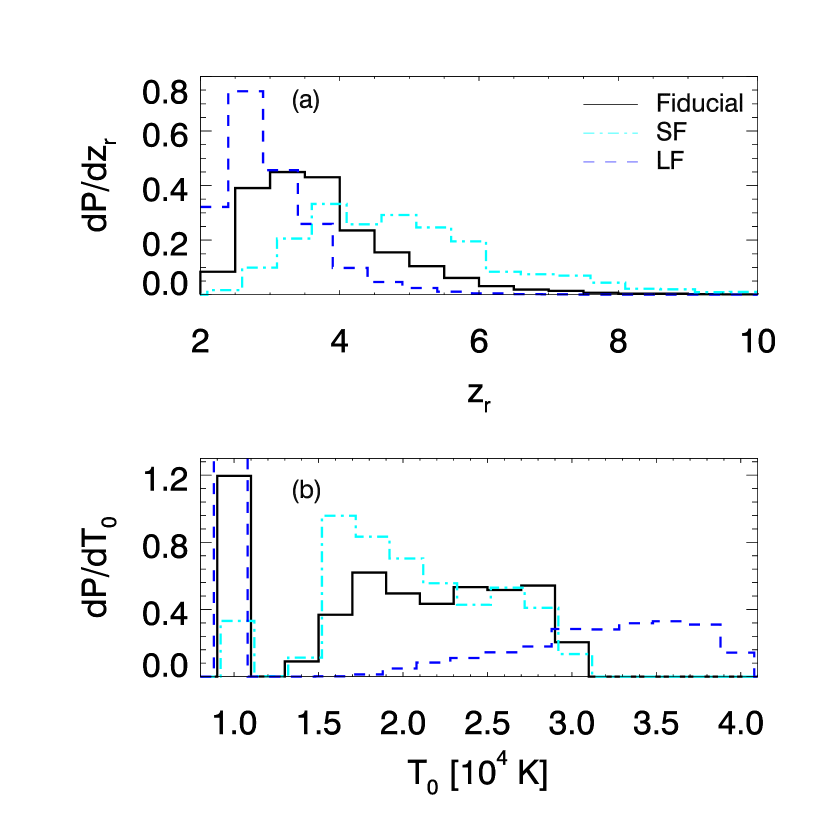
Figure 2.— Panel (a): He II reionization redshift distribution for the fiducial, SF, and LF models. Panel (b): Temperature distribution at $z=3$ for the same reionization models in (a). For illustrative clarity, the SF and LF models are shifted in the $z_{r}$-direction by +0.1 and -0.1 respectively in (a), and in the $T_{0}$-direction by +200 K and -200 K in (b).

We construct realizations of the $T_{0}$ and $\gamma$ fields in each of the models discussed in the previous section. We use a $80\,h^{-1}\,{\rm Mpc}$ comoving box, and $512^{3}$ mesh points. This boxsize is convenient for overlaying on the cosmological simulation which we will describe in § 5. Throughout, we average the statistics in the fiducial, LF, and LS models over five independent realizations, in order to reduce scatter owing to the small number of He III bubbles in our $80\,h^{-1}\,{\rm Mpc}$ simulation box. In the other models, the bubble distribution is sampled sufficiently well with a single realization.

With the numerical models in hand, we proceed to measure the probability distribution of the temperature field. We first examine in Fig. 2a the probability distribution of He II reionization redshifts, in analogy with Fig. 1a. This figure is constructed by recording the redshift at which each pixel in the simulation is first engulfed by an expanding He III bubble. We only plot our fiducial, SF, and LF models, since the other models have temperature distributions that are similar to that of the LF model. One can see that He II reionization is quite extended, and that these simple models are each consistent with incomplete He II reionization near $z\sim 3$. Our models are essentially Monte-Carlo versions of the Madau et al. (1999) calculation and are consistent with these earlier calculations.

The resulting temperature distributions at $z=3$ are shown in Fig. 2b. In our models, we assume that the background IGM, in which only H I/He I is reionized, has a uniform temperature at $T_{0}=10^{4}\mbox{ K}$, as justified in § 3. We additionally assume a uniform $\gamma=1.4$ for the background IGM. In the figure, one can clearly see the bimodal temperature distribution that results from incomplete He II reionization. The $\gamma$ distribution exhibits a similar bimodal distribution, with $\gamma\sim 1$ inside He III regions, and $\gamma=1.4$ in the background IGM. The temperature distributions are quite broad, with r.m.s. fluctuation amplitudes of $\sigma_{T_{0}}/\langle T_{0}\rangle$ = 0.24, 0.33, and 0.58 ($\sigma_{T_{0}}$ = $4.8\times 10^{3}$ K, $6.4\times 10^{3}$ K, and $1.2\times 10^{4}$ K) in the SF, fiducial, and LF models, respectively. Note that the higher temperatures of the hot regions in the LF model are not a consequence of that model’s reionization history, but rather because we chose a larger $T_{r}$ to maximize fluctuations. Compared to the results from § 3, we see that temperature fluctuations from incomplete He II reionization can be as much as a factor of 10 larger than that from extended H I reionization.

The temperature distributions shown in Fig. 2b are each distributions at $z=3$ in different models, but they also roughly represent the fluctuations during different stages of reionization. The filling factor of He III regions, $Q$, is indicated by the area under the hot component of the temperature distribution. In the LF model, $Q$ is about 0.5 at $z=3$. Here, the amplitude of temperature fluctuations is maximal, as the hot and cold regions occupy comparable fractions of space. On the other hand, in the SF and fiducial models, reionization is considerably more complete. The temperature distribution is dominated by hot regions by $z=3$, and the fluctuations are smaller. At a higher redshift, He II reionization is less complete in the fiducial and SF models, and the temperature distributions in these models will be similar to that in the LF model at $z=3$.

4.3. Power Spectrum of Temperature Fluctuations

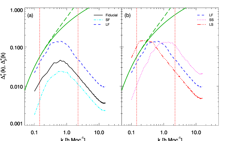
Figure 3.— Panel (a): 3-dimensional power spectrum of $T_{0}$ at $z=3$ in the fiducial, LF, and SF models. Panel (b): 3-dimensional power spectrum of $T_{0}$ at $z=3$ in the SS and LS models, with the LF model repeated for comparison. The linear and non-linear matter power spectrum are shown as the green solid and dashed lines, respectively. The vertical red dotted lines indicate the range of scales probed by SDSS.

The temperature distributions presented above are informative, but they tell us nothing about the characteristic scale of the temperature fluctuations. To investigate this, we measure the 3-dimensional power spectrum of the temperature field, $T_{0}$, from our simulations. In Fig. 3 we show the dimensionless power spectrum, $\Delta_{T}^{2}(k)\propto k^{3}P_{T}(k)$, for each of the five models we consider. Each power spectrum shows a well defined characteristic scale, with the power spectrum growing as $k^{3}$ on large scales, and falling as $k^{-1}$ on small scales. The large and small scales trends in $\Delta_{T}^{2}(k)$ are a natural consequence of our model in which the source positions are uncorrelated (see below for comments on this approximation). The assumptions that the bubbles have a well defined boundary, and that $T_{0}$ within each bubble is uniform, also contribute to the trends seen in $\Delta_{T}^{2}(k)$. The characteristic bubble size is set by (see Eqs. 6 and 7) the break in the luminosity function, $L_{*}$, the quasar spectrum, and the quasar lifetime, $t_{q}$. The characteristic comoving scale in the fiducial, SF, and LF models is $R_{*}\sim 5\,h^{-1}\,{\rm Mpc}$, while it is $R_{*}\sim 11\,h^{-1}\,{\rm Mpc}$ in the LS model, and $R_{*}\sim 2\,h^{-1}\,{\rm Mpc}$ in the SS model.

Two simplifying assumptions in our model may cause the characteristic scale to be underestimated. First, our model does not take into account quasar clustering, and so we tend to underestimate the chance that ionized bubbles around neighboring quasars will overlap to form large ionized regions. Assuming a quasar bias $b_{q}=4$ (extrapolated from Croom et al. 2005), we find that clustering enhances the average number of sources inside an ionized region by a factor of $\sim 3$ over that of a uniform distribution. However, even when the effect of clustering is included, there are on average $<1$ additional active sources inside an ionized region of size $R\sim 10\,h^{-1}\,{\rm Mpc}$. Therefore, the clustering of active sources can safely be ignored. Quasar clustering will also lead to the clustering and overlap of fossil ionized regions. In this case, neglecting clustering may cause the typical volume of hot regions to be underestimated by as much as a factor of 3. It is therefore prudent to investigate models spanning a wide range of characteristic scales, as we have done. The second simplification in our model is in our treatment of multiple ionizing sources. When the ionization fronts of two or more bubbles overlap, the resulting large ionized region will expand so as to conserve ionizing photons coming from the multiple sources inside the combined region. We neglect this subtlety in our modeling, noting that the probability for overlap is not significant around $Q=0.5$, when temperature fluctuations are largest.

We aim to explore the effects of temperature fluctuations on the statistics of the absorption in the Ly$\alpha$ forest. Since in the standard picture of the forest most structure derives from gravitational instability, it is instructive to compare temperature fluctuations with density fluctuations. Which is a more important source of structure in the Ly$\alpha$ forest, temperature or density fluctuations? We address this question in Fig. 3, where we include curves indicating the linear matter power spectrum, and the Peacock & Dodds (1996) fit for the non-linear power spectrum. This may not be exactly the relevant comparison: for instance, the optical depth to Ly$\alpha$ absorption scales with matter density as $(1+\delta)^{2}$, while it only varies with temperature as $(1+\delta_{T_{0}})^{-0.7}$. Density fluctuations of a given amplitude are therefore amplified into larger optical depth fluctuations than temperature fluctuations of the same amplitude. Nonetheless, the comparison is suggestive. Fig. 3 illustrates that on small scales, $k\gtrsim 1\,h\,{\rm Mpc^{-1}}$, the density power is at least $1-2$ orders of magnitude larger than the temperature power in all models considered. On these scales, fluctuations in the density field will be the more important source of structure in the Ly$\alpha$ forest. On the other hand, on large scales, the temperature power may be comparable, or even dominant, in comparison to the density power. For instance, in the LS model, the temperature power is actually larger than the density power for $k\lesssim 0.3\,h\,{\rm Mpc^{-1}}$.

Our results seem to suggest that temperature fluctuations may be an important source of structure in the Ly$\alpha$ forest on large scales. There are, however, a few caveats to this intuition. First, as mentioned above, the optical depth scales more strongly with density than temperature. Second, current flux power spectrum measurements do not probe very large scales, as illustrated by the red dotted lines in Fig. 3, which show the range of scales probed by SDSS observations. This suggests that if the characteristic scale of the temperature fluctuations is large, much of the effect will be on scales larger than that probed by current measurements. Finally, it is important to keep in mind, that the Ly$\alpha$ forest provides a 1-d skewer through the IGM. As a result, the power spectrum of fluctuations along a line of sight, on large scales, includes aliased power from small wavelength modes transverse to the line of sight. This may tend to wash out some of the signal from temperature fluctuations on large scales.

5. Impact of Temperature Fluctuations on the Flux Power Spectrum

We now arrive at the heart of our study: how do the temperature fluctuations, described in the previous section, impact the flux power spectrum? To answer this question, we turn to cosmological simulations. We combine the realizations of the $T_{0}$ and $\gamma$ fields discussed in the previous section with the density and peculiar velocity fields from a cosmological simulation. We then extract absorption spectra from the simulation, and measure the flux power with and without temperature fluctuations.

The cosmological simulation we use is a Hydro-Particle-Mesh (HPM) simulation (Gnedin & Hui 1998; Heitmann et al. 2005; Lidz et al. 2006; Habib et al. 2005, in prep.), with $2\times 512^{3}$ particles and $512^{3}$ mesh-points in an $80\,h^{-1}\,{\rm Mpc}$ box. For our purposes, we want a simulation box that is large enough to sample the He III bubble distribution, while resolving the pressure-smoothing and thermal broadening scales. Our simulation represents a compromise between these requirements. The resolution is inadequate for detailed predictions, as shown in the convergence studies presented in the Appendix of Lidz et al. (2006). Furthermore, the accuracy of HPM has been criticized in the literature (e.g. Viel et al., 2005a). However, our present goal is only to investigate how the flux power spectrum differs with and without temperature fluctuations, rather than to make a detailed comparison with data. For this limited purpose, we believe our simulation is adequate. One further caveat is that the gas pressure force, as calculated in our HPM simulation, depends on the thermal history of the IGM. In principle, we should use the fluctuating temperature field in our models to calculate the gas pressure in our HPM simulation. However, we ignore this effect and use HPM simulations calculated with a uniform temperature, including the temperature fluctuations only when we construct the artificial Ly$\alpha$ forest spectra. The flux power spectrum, particularly on SDSS scales, depends rather weakly on gas pressure-smoothing (McDonald et al., 2005b; Viel & Haehnelt, 2006), and so this is probably a good approximation.

We extract artificial spectra at $z=3$ from the HPM simulation box in the usual way (see Eq. 1), incorporating peculiar velocities and thermal broadening. This is done for each of our five models, and we compare the flux power spectrum in the fluctuating temperature model with that in a similar model without temperature fluctuations. In the models without temperature fluctuations, $T_{0}$ and $\gamma$ are each set to their global averages in the corresponding models that include temperature fluctuations. In each case, we normalize the quantity $A_{\tau}$ in Eq. 1 to match the observed mean transmitted flux at $z=3$, which we take to be $\langle F\rangle=0.68$, close to the value measured by McDonald et al. (2000).

The results of this calculation are shown in Fig. 4 and Fig. 5, where we parameterize the effect of temperature fluctuations by the fractional difference in the flux power spectrum between a fluctuating temperature model and a no fluctuations model. The first feature to notice is simply that the effect of temperature fluctuations on the flux power spectrum is quite small on all scales examined. Closer examination reveals that the flux power spectrum is boosted on large scales and on small scales compared to equivalent models without temperature fluctuations, while there is a very slight suppression on intermediate scales. We will discuss each effect in turn.

The first effect is due to increased structure in the forest on large scales, contributed by the hot, isothermal He III bubbles. The flux power is boosted on large scales because the flux transmission is sensitive to the temperature-dependent recombination coefficient, and the spatially fluctuating temperature-density relation. In Fig. 4, concentrating on large scales for the moment, we study the effect for models with varying levels of temperature fluctuations: the fiducial, SF, and LF models. Specifically, we compare the fractional difference between the flux power spectrum with and without temperature fluctuations and the 1-$\sigma$ error bars on the SDSS measurements of McDonald et al. (2006). The fractional difference between the models is always smaller than the 1-$\sigma$ SDSS errors. The difference is only at the $5\%$ level on the largest scales probed in the LF model. The effect also appears to diminish rather quickly with decreasing temperature fluctuation strength, as illustrated by the other two models in the figure.

In Fig. 5, we show the same comparison for models in which we vary the characteristic scale of the temperature fluctuations: the SS, LF, and LS models. Each of these models has approximately the same fluctuation strength, and only differ in their characteristic scale. In this case, the effect can be as large as $\sim 10\%$ on the largest scales probed, comparable to the SDSS 1-$\sigma$ error bars at this redshift. In the models where the characteristic scale of the temperature fluctuations is smaller, the effect on the flux power spectrum is smaller. This appears to be consistent with the interpretation suggested in § 4.3: density fluctuations generally swamp temperature fluctuations, unless the temperature fluctuations have a large characteristic scale.

The next effect is a boost in the small scale power, which is the result of thermal broadening. The figures illustrate that the models with temperature fluctuations typically have $\sim 20\%$ more power on scales of $k\sim 0.1$ s/km than corresponding models with a uniform $T_{0}$ and $\gamma$. In Fig. 4 and 5, we compare this boost in small scale power to the 1-$\sigma$ statistical error-bars on the measurement of Croft et al. (2002), which is the most precise measurement to date on these scales. The enhanced small scale power in the models with temperature fluctuations can be understood as follows. On small scales, the power spectrum in a fluctuating temperature model will approximately be a filling-factor weighted average of the power spectrum of hot regions and that of cold regions. Roughly speaking, the power spectrum on small scales is exponentially suppressed with increasing temperature (Zaldarriaga et al., 2001a). The weighted average we mention, and hence the power spectrum on small scales in fluctuating temperature models, is therefore dominated by the cold regions. The fluctuating temperature model will then have more small scale power than a uniform temperature model with the same mean temperature as the fluctuating model.

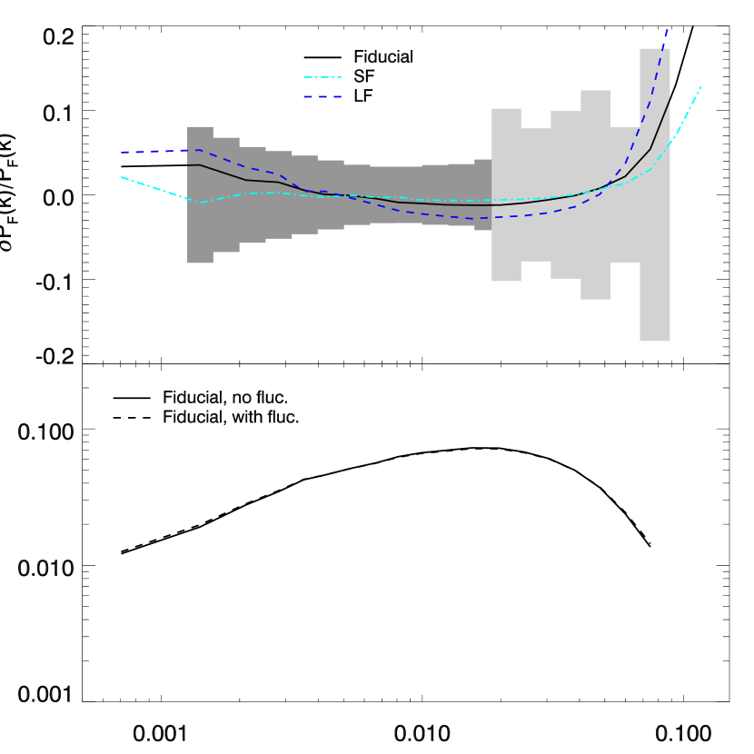
Figure 4.— Top: Fractional difference in the $z=3$ flux power spectrum between simulations with and without temperature fluctuations. The fiducial, SF, and LF models are plotted with the 1-$\sigma$ fractional errors from McDonald et al. (2006) and Croft et al. (2002) (dark and light gray shaded areas, respectively). Bottom: Flux power spectrum with and without temperature fluctuations in the fiducial model.

Finally, there is a slight suppression in the flux power on intermediate scales, typically around a few percent. This suppression occurs on scales in which the temperature field has little power, and on scales too large for thermal broadening to have an effect. The suppression is likely a consequence of the fact that the normalization $A_{\tau}$ required to match the observed mean transmitted flux is slightly smaller in models with a fluctuating temperature field. The smaller $A_{\tau}$ in the fluctuating temperature models implies that density fluctuations of a given amplitude are translated into lesser optical depth fluctuations on intermediate scales.

One might expect temperature fluctuations to have a larger effect at high redshift, when the amplitude of density fluctuations is smaller. We test this by considering a model that, at $z=4$, has very similar temperature fluctuations to those in our LF model at $z=3$. The parameters of this model, which we call LF4, are detailed in Table 1. We find that the effect, again parameterized by the fractional difference between the models with and without temperature fluctuations, is only a couple percent larger on large scales in the LF4 model. Even though the effect is larger at $z=4$, it is less significant in the sense that the statistical errors on the SDSS measurement are larger at $z=4$ than at $z=3$.

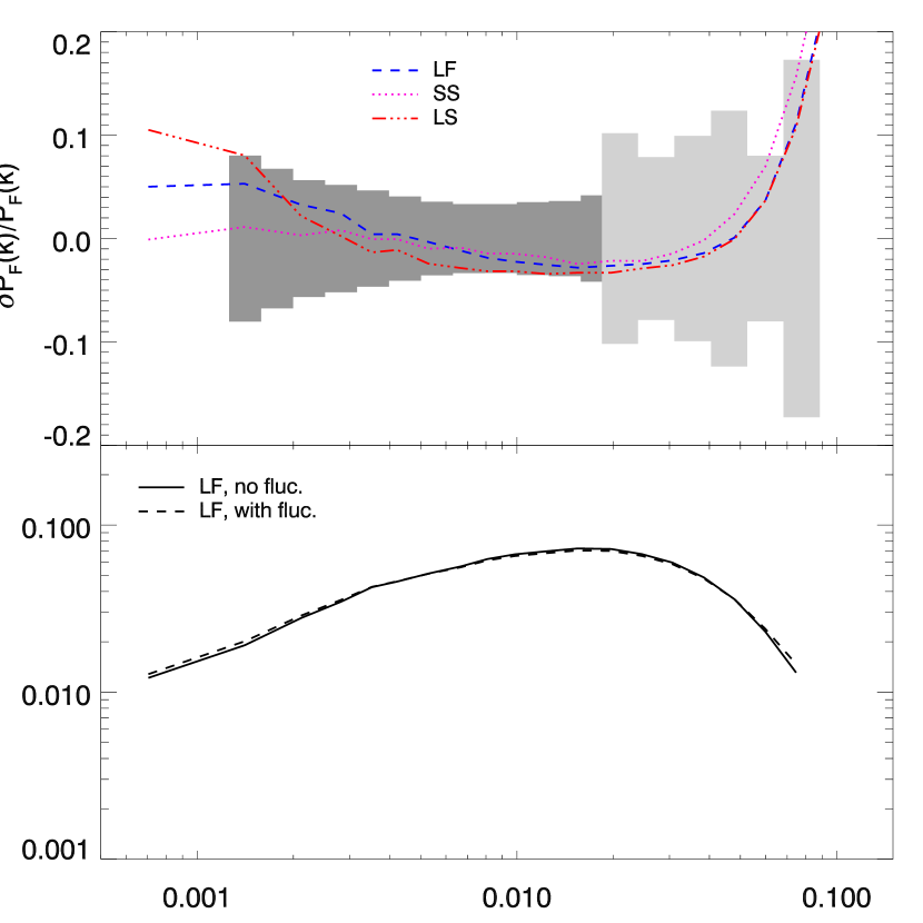
Figure 5.— Top: Similar to Fig. 4 but for the LF, SS, and LS models. Bottom: Flux power spectrum with and without temperature fluctuations in the LF model.

6. Conclusion

In this paper, we have estimated the level of temperature fluctuations expected in the IGM at $z\sim 3$ from extended H I reionization and incomplete He II reionization. We find that the temperature fluctuations from extended H I reionization should be quite small, $\sigma_{T_{0}}/\langle T_{0}\rangle\lesssim 5\%$, while the fluctuations from incomplete He II reionization might be as large as $\sim 50\%$. These fluctuations should have only a small effect on the flux power spectrum: on large scales, $k\sim 0.001\;{\rm s/km}$, temperature fluctuations lead to an increase in the $z=3$ flux power spectrum by at most $\sim 10\%$. On small scales, $k\sim 0.1\;{\rm s/km}$, fluctuations in the thermal broadening scale boost the power by $\sim 20\%$.

Further study is required to quantify the effects of temperature fluctuations on cosmological parameter constraints. In particular, note that in the LS model (see Fig. 5), the effect of temperature fluctuations are at, or larger than, the 1-$\sigma$ level over several independent data points. A detailed investigation will require a multi-parameter fit to the observed data (see McDonald et al., 2005b), which is outside the scope of the present paper. However, we can anticipate the results of a more detailed investigation by comparing with the effects of UV background fluctuations, as studied in McDonald et al. (2005a, b). Fluctuations in the UV background and temperature fluctuations have a similar influence on the amplitude and shape of the flux power spectrum, at least on large scales (see Fig. 12 of McDonald et al. 2005b). McDonald et al. (2005b) included the effect of UV background fluctuations in a multi-parameter fit, and found little effect ($\lesssim 1\%$) on the inferred values of the amplitude and slope of the linear power spectrum. The general reason for this insensitivity is that the effective errors on the flux power spectrum are larger than the raw statistical errors on the data, after McDonald et al. (2005b) marginalize over other, more significant, effects. Similarly, we do not expect temperature fluctuations to have a substantial effect on the values of the amplitude and slope of the linear power spectrum.

For the purpose of cosmological parameter estimation, it would be instructive to know whether the effect of temperature fluctuations is degenerate with any parameters describing the Ly$\alpha$ forest. As we mentioned in the previous paragraph, the effect of temperature fluctuations may be degenerate with those of UV background fluctuations on large scales. However, they have different effects on small scales. Additionally, inspecting, e.g. Fig. 13 of McDonald et al. (2005b) (see also Viel & Haehnelt, 2006), shows that the boost in the flux power on large and small scales expected from temperature fluctuations is not closely mimicked by changing any single modeling parameter. In principle, this means that the effect of temperature fluctuations is likely distinguishable from other effects. The redshift evolution of the effect potentially provides an additional diagnostic. However, even though the number of quasar spectra will likely more than double by the time SDSS is finished, detecting temperature fluctuations in the flux power spectrum will remain a challenge owing to the smallness of the effect.

Numerous improvements could be made in our simple modeling. First, we place quasars at random positions in our simulation box, which ignores quasar clustering. This effect is already discussed in § 4.3. Here, we note that since quasars are very sparse sources, ignoring source clustering is a much better approximation than in the case that the sources are galaxies, in which case this approximation is quite poor (Furlanetto et al., 2004). Furthermore, in reality, quasars should reside in very massive halos, rather than at random positions. As a result, we ignore the fact that very close to the quasar the gas will be overdense, tending to cancel out the enhanced transmission owing to the hot He III bubble around the quasar. The bubbles are, however, $\sim 10\,h^{-1}\,{\rm Mpc}$ in size, over which the density contrast will be small.

In modeling temperature fluctuations (the ‘thermal proximity effect’), we also ignored the ‘radiation proximity effect’. In reality the intensity of ionizing radiation will be enhanced over that of the radiation background close to an active quasar (e.g. Scott et al., 2002; Rollinde et al., 2005). Nearby dead quasars, ‘light echos’ of enhanced radiation will remain, propagating out into the IGM (Croft, 2004). These effects are ignored in our modeling, and the radiation background is treated as uniform. In any case, the effects of the radiation proximity effect should be small compared to that from temperature fluctuations. This is because the radiation proximity effect has a characteristic time scale of $t_{q}\sim 10^{7}$ yrs, short compared to the characteristic time scale of temperature fluctuations, $t_{\rm cool}\sim 10^{9}$ yrs. Here, we define the cooling time $t_{\rm cool}$ to be the time it takes for a gas element to cool to half its original temperature assuming only adiabatic cooling. The longer characteristic time scale, and the fact that temperature fluctuations and the radiation proximity effect have similar physical characteristic scales, imply that a much larger fraction of space is affected by temperature fluctuations than by the radiation proximity effect.

Additionally, we used a simplified ‘light bulb’ model for quasar activity, in which each quasar shines at constant luminosity for the duration of its lifetime, $t_{q}$, and emit no light thereafter. In reality, this is probably a poor approximation to the quasar light curve, since quasars likely spend extended periods at low luminosity, going into or coming out of their peak luminosity phase (Hopkins et al., 2005; Springel et al., 2005). Finally, quasars may launch large outflows (e.g. Scannapieco & Oh, 2004; Di Matteo et al., 2005), which could also modify the absorption in their vicinity.

In spite of all of these possible complications, we strove to cover a wide range in the amplitude and scale of temperature fluctuations in our analysis. It is unlikely that the problems discussed above will lead to an effect that lies far outside the range probed by our study. It should therefore be a fairly secure conclusion that temperature fluctuations do not significantly impact the Ly$\alpha$ forest flux power spectrum on large scales. Our results provide additional support for the Ly$\alpha$ forest as a robust probe of cosmology.

Even though temperature fluctuations seem to have a small effect on the flux power spectrum, they may have a larger effect on other observables of the Ly$\alpha$ forest. The flux power spectrum, while being the best measured statistic in the Ly$\alpha$ forest, may be a poor statistic to use in searching for temperature fluctuations. There have been several searches for temperature fluctuations in the Ly$\alpha$ forest with wavelet analyses (Theuns et al., 2002b; Zaldarriaga, 2002). These searches have failed to detect temperature fluctuations, but have been carried out using only very small data samples. It would be interesting to investigate the expected signal from these searches given our modeling. A related statistic that might be sensitive to temperature fluctuations is the Ly$\alpha$ forest ‘tri-spectrum’, as defined in Zaldarriaga et al. (2001b) (see also Fang & White 2004). This statistic measures the scatter in the small scale power, as a function of scale, from region to region in the IGM. We might, therefore, expect a larger tri-spectrum in our models with temperature fluctuations than in models with no temperature fluctuations.

One final point is that if He II reionization is underway at $z=3$, this might cause biases in estimates of the IGM temperature from the flux power spectrum, and the ionizing background derived from the Ly$\alpha$ forest proximity effect. The enhancement we find in the flux power spectrum on small scales might imply a slight bias in measurements of the IGM temperature from the small scale flux power spectrum (e.g. Zaldarriaga et al., 2001a), and other similar measurements. A crude estimate of the bias is as follows. Approximately, thermal broadening suppresses the flux power exponentially so that $P_{F}(k)\propto\exp(-k^{2}\sigma^{2})$, where $\sigma^{2}=k_{\rm b}T/m_{\rm H}$, and $k_{\rm b}$ is Boltzmann’s constant. We found that temperature fluctuations increase $P_{F}(k)$ at $k=0.1$ s/km by $20\%$, which thereby implies a $\sim 10\%$ underestimate of the temperature in models that assume a uniform temperature. We caution, however, that the mean temperature is an incomplete description of the IGM thermal state in the presence of inhomogeneous reionization and/or large quantities of hot, shocked gas. Temperature fluctuations may also bias estimates of the ionizing background from the quasar proximity effect, which assumes that the IGM is at the cosmic mean temperature close to the quasar. We are investigating this, and other possible biases in the constraints from the proximity effect, using radiative transfer simulations.

AL thanks Katrin Heitmann and Salman Habib for their collaboration in producing the HPM simulation used in this analysis. We thank the anonymous referee for useful comments on our manuscript. We also thank Scott Burles, Steve Furlanetto, John Huchra, and Peng Oh for useful discussions on these, and related topics. This work was supported in part by NSF grants ACI 96-19019, AST 00-71019, AST 02-06299, AST 03-07690, and NASA ATP grants NAG5-12140, NAG5-13292, and NAG5-13381. Some of the simulations were performed at the Center for Parallel Astrophysical Computing at the Harvard-Smithsonian Center for Astrophysics.

References

- Abel & Haehnelt (1999) Abel, T. & Haehnelt, M. G. 1999, ApJ, 520, L13
- Babich & Loeb (2006) Babich, D. & Loeb, A. 2006, ApJ, 640, 1
- Barkana & Loeb (2004) Barkana, R. & Loeb, A. 2004, ApJ, 609, 474
- Bi & Davidsen (1997) Bi, H. & Davidsen, A. F. 1997, ApJ, 479, 523
- Bond et al. (1991) Bond, J. R., Cole, S., Efstathiou, G., & Kaiser, N. 1991, ApJ, 379, 440
- Bond & Wadsley (1997) Bond, J. R. & Wadsley, J. W. 1997, in ASP Conf. Ser. 123: Computational Astrophysics; 12th Kingston Meeting on Theoretical Astrophysics, 323–+
- Boyle et al. (1988) Boyle, B. J., Shanks, T., & Peterson, B. A. 1988, MNRAS, 235, 935
- Bryan et al. (1999) Bryan, G. L., Machacek, M., Anninos, P., & Norman, M. L. 1999, ApJ, 517, 13
- Cen et al. (1994) Cen, R., Miralda-Escude, J., Ostriker, J. P., & Rauch, M. 1994, ApJ, 437, L9
- Croft (2004) Croft, R. A. C. 2004, ApJ, 610, 642
- Croft et al. (1999) Croft, R. A. C., Hu, W., & Davé, R. 1999, Physical Review Letters, 83, 1092
- Croft et al. (2002) Croft, R. A. C., Weinberg, D. H., Bolte, M., Burles, S., Hernquist, L., Katz, N., Kirkman, D., & Tytler, D. 2002, ApJ, 581, 20
- Croft et al. (1998) Croft, R. A. C., Weinberg, D. H., Katz, N., & Hernquist, L. 1998, ApJ, 495, 44
- Croom et al. (2005) Croom, S. M., et al. 2005, MNRAS, 356, 415
- Croom et al. (2004) Croom, S. M., Smith, R. J., Boyle, B. J., Shanks, T., Miller, L., Outram, P. J., & Loaring, N. S. 2004, MNRAS, 349, 1397
- Davé et al. (1999) Davé, R., Hernquist, L., Katz, N., & Weinberg, D. H. 1999, ApJ, 511, 521
- Di Matteo et al. (2005) Di Matteo, T., Springel, V., & Hernquist, L. 2005, Nature, 433, 604
- Fan et al. (2002) Fan, X., Narayanan, V. K., Strauss, M. A., White, R. L., Becker, R. H., Pentericci, L., & Rix, H.-W. 2002, AJ, 123, 1247
- Fan et al. (2001) Fan, X., et al. 2001, AJ, 121, 54
- Fang & White (2004) Fang, T. & White, M. 2004, ApJ, 606, L9
- Furlanetto et al. (2006) Furlanetto, S. R., McQuinn, M., & Hernquist, L. 2006, MNRAS, 365, 115
- Furlanetto & Oh (2005) Furlanetto, S. R. & Oh, S. P. 2005, MNRAS, 363, 1031
- Furlanetto et al. (2004) Furlanetto, S. R., Zaldarriaga, M., & Hernquist, L. 2004, ApJ, 613, 1
- Gnedin & Hui (1998) Gnedin, N. Y. & Hui, L. 1998, MNRAS, 296, 44
- Heitmann et al. (2005) Heitmann, K., Ricker, P. M., Warren, M. S., & Habib, S. 2005, ApJS, 160, 28
- Hernquist et al. (1996) Hernquist, L., Katz, N., Weinberg, D. H., & Miralda-Escudé, J. 1996, ApJ, 457, L51+
- Hopkins et al. (2005) Hopkins, P. F., Hernquist, L., Cox, T. J., Di Matteo, T., Robertson, B., & Springel, V. 2005, ApJ, 630, 716
- Hui & Gnedin (1997) Hui, L. & Gnedin, N. Y. 1997, MNRAS, 292, 27
- Hui et al. (1997) Hui, L., Gnedin, N. Y., & Zhang, Y. 1997, ApJ, 486, 599
- Hui & Haiman (2003) Hui, L. & Haiman, Z. 2003, ApJ, 596, 9
- Lacey & Cole (1993) Lacey, C. & Cole, S. 1993, MNRAS, 262, 627
- Lidz et al. (2006) Lidz, A., Heitmann, K., Hui, L., Habib, S., Rauch, M., & Sargent, W. L. W. 2006, ApJ, 638, 27
- Madau et al. (1999) Madau, P., Haardt, F., & Rees, M. J. 1999, ApJ, 514, 648
- McDonald et al. (2000) McDonald, P., Miralda-Escudé, J., Rauch, M., Sargent, W. L. W., Barlow, T. A., Cen, R., & Ostriker, J. P. 2000, ApJ, 543, 1
- McDonald et al. (2005a) McDonald, P., Seljak, U., Cen, R., Bode, P., & Ostriker, J. P. 2005a, MNRAS, 360, 1471
- McDonald et al. (2005b) McDonald, P., et al. 2005b, ApJ, 635, 761
- McDonald et al. (2006) McDonald, P., et al. 2006, ApJS, 163, 80
- Meiksin (2005) Meiksin, A. 2005, MNRAS, 356, 596
- Meiksin & White (2004) Meiksin, A. & White, M. 2004, MNRAS, 350, 1107
- Miralda-Escude et al. (1996) Miralda-Escude, J., Cen, R., Ostriker, J. P., & Rauch, M. 1996, ApJ, 471, 582
- Miralda-Escude & Rees (1994) Miralda-Escude, J. & Rees, M. J. 1994, MNRAS, 266, 343
- Muecket et al. (1996) Muecket, J. P., Petitjean, P., Kates, R. E., & Riediger, R. 1996, A&A, 308, 17
- Nusser & Haehnelt (1999) Nusser, A. & Haehnelt, M. 1999, MNRAS, 303, 179
- Peacock & Dodds (1996) Peacock, J. A. & Dodds, S. J. 1996, MNRAS, 280, L19
- Pei (1995) Pei, Y. C. 1995, ApJ, 438, 623
- Richards et al. (2005) Richards, G. T., et al. 2005, MNRAS, 360, 839
- Rollinde et al. (2005) Rollinde, E., Srianand, R., Theuns, T., Petitjean, P., & Chand, H. 2005, MNRAS, 610
- Scannapieco & Oh (2004) Scannapieco, E. & Oh, S. P. 2004, ApJ, 608, 62
- Scott et al. (2002) Scott, J., Bechtold, J., Morita, M., Dobrzycki, A., & Kulkarni, V. P. 2002, ApJ, 571, 665
- Seljak et al. (2005) Seljak, U., et al. 2005, Phys. Rev. D, 71, 103515
- Shapiro & Giroux (1987) Shapiro, P. R. & Giroux, M. L. 1987, ApJ, 321, L107
- Sokasian et al. (2002) Sokasian, A., Abel, T., & Hernquist, L. 2002, MNRAS, 332, 601
- Sokasian et al. (2003) Sokasian, A., Abel, T., Hernquist, L., & Springel, V. 2003, MNRAS, 344, 607
- Sokasian et al. (2004) Sokasian, A., Yoshida, N., Abel, T., Hernquist, L., & Springel, V. 2004, MNRAS, 350, 47
- Springel et al. (2005) Springel, V., Di Matteo, T., & Hernquist, L. 2005, MNRAS, 361, 776
- Theuns et al. (1999) Theuns, T., Leonard, A., Schaye, J., & Efstathiou, G. 1999, MNRAS, 303, L58
- Theuns et al. (2002a) Theuns, T., Schaye, J., Zaroubi, S., Kim, T., Tzanavaris, P., & Carswell, B. 2002a, ApJ, 567, L103
- Theuns et al. (2002b) Theuns, T., Zaroubi, S., Kim, T., Tzanavaris, P., & Carswell, R. F. 2002b, MNRAS, 332, 367
- Tytler et al. (2004) Tytler, D., et al. 2004, ApJ, 617, 1
- Viel & Haehnelt (2006) Viel, M. & Haehnelt, M. G. 2006, MNRAS, 365, 231
- Viel et al. (2004) Viel, M., Haehnelt, M. G., & Springel, V. 2004, MNRAS, 354, 684
- Viel et al. (2005a) —. 2006, MNRAS, 367, 1655
- Viel et al. (2005b) Viel, M., Lesgourgues, J., Haehnelt, M. G., Matarrese, S., & Riotto, A. 2005b, Phys. Rev. D, 71, 063534
- Zaldarriaga (2002) Zaldarriaga, M. 2002, ApJ, 564, 153
- Zaldarriaga et al. (2001a) Zaldarriaga, M., Hui, L., & Tegmark, M. 2001a, ApJ, 557, 519
- Zaldarriaga et al. (2003) Zaldarriaga, M., Scoccimarro, R., & Hui, L. 2003, ApJ, 590, 1
- Zaldarriaga et al. (2001b) Zaldarriaga, M., Seljak, U., & Hui, L. 2001b, ApJ, 551, 48
- Zhang et al. (1995) Zhang, Y., Anninos, P., & Norman, M. L. 1995, ApJ, 453, L57+