Adaptive Mesh Refinement Simulations of the Ionization Structure and Kinematics of Damped Ly$\alpha$ Systems with Self-consistent Radiative Transfer

Abstract

We use high resolution Eulerian hydrodynamics simulations to study kinematic properties of the low ionization species in damped Ly$\alpha$ systems at redshift $z=3$. Our adaptive mesh refinement simulations include most key ingredients relevant for modeling neutral gas in high-column density absorbers: hydrodynamics, gravitational collapse, continuum radiative transfer above the hydrogen Lyman limit and gas chemistry, but no star formation. We model high-resolution Keck spectra with unsaturated low ion transitions in two Si II lines ($1526$ and $1808{A}$), and compare simulated line profiles to the data from the SDSS DLA survey.

We find that with increasing grid resolution the models show a trend in convergence towards the observed distribution of HI column densities. While in our highest resolution model we recover the cumulative number of DLAs per unit absorption distance, none of our models predicts DLA velocity widths as high as indicated by the data, suggesting that feedback from star formation might be important. At $z=3$ a non-negligible fraction of DLAs with column densities below $10^{21}{\rm\,cm}^{-2}$ is caused by filamentary structures in more massive halo environments. Lower column density absorbers with $N_{\rm HI}<10^{21.4}{\rm\,cm}^{-2}$ are sensitive to changes in the UV background resulting in a $10\%$ reduction of the cumulative number of DLAs for twice the quasar background relative to the fiducial value, and nearly a $40\%$ reduction for four times the quasar background. We find that the mass cut-off below which a large fraction of dwarf galaxies cannot retain gas after reionization is $\sim 7\times 10^{7}{\rm\,M_{\odot}}$, lower than the previous estimates. Finally, we show that models with self-shielding commonly used in the literature produce significantly lower DLA velocity widths than the full radiative transfer runs which essentially render these self-shielded models obsolete.

1. Introduction

Damped Ly$\alpha$ absorbers (DLAs) are an excellent tool for probing structure formation in the early Universe. By definition DLAs are systems with neutral hydrogen column densities above $2\times 10^{20}{\rm\,cm}^{-2}$, and for many years they have been linked to forming protogalaxies at high redshifts. With high resolution spectrography, DLAs can shed light on physical processes and substructure within individual young galaxies. However, the exact nature of host absorbers has been debated for many years.

From metal-line kinematic analysis of absorption line widths and profile asymmetries Prochaska & Wolfe (1997) concluded that the observed DLA population can be best explained with a model in which absorption is caused by rapidly rotating (${v_{\rm circ}}\sim 225{\rm\,km\,s^{-1}}$) cold thick ($h\sim 0.3R$) disks which have already assembled at high redshifts, and ruled out the competing models in which DLAs are small (${v_{\rm circ}}\leq 100{\rm\,km\,s^{-1}}$) protogalaxies in the process of hierarchical merger. However, in most models of hierarchical structure formation it is extremely difficult to have an abundant population of such massive disks at $z\sim 3-4$.

On the other hand, in the high-resolution (1 kpc spatial and $5\times 10^{6}{\rm\,M_{\odot}}$ mass resolution) SPH simulations of a small number of high-redshift galaxies Haehnelt et al. (1998) showed that irregular protogalactic clumps with ${v_{\rm circ}}\sim 100{\rm\,km\,s^{-1}}$ can reproduce the observed velocity width distribution and absorption profile asymmetries very well, without the need to invoke rapidly rotating massive disks. In their models large velocity widths are caused by a mixture of rotation, random motions, infall, and merging, and the resulting picture is fully consistent with most standard hierarchical structure formation scenarios. Despite having achieved very high numerical resolution, this simulation features a small volume size (2 Mpc) and may not be representative of a typical DLA absorber in the cosmological context. Another shortcoming of Haehnelt et al. (1998) paper is that their models do not include radiative transfer of the ultraviolet background (UVB) instead assuming simple self-shielding above a critical density, an assumption that directly affects the cross-section of DLAs. In our paper we are going to address this issue in detail.

Simulations with larger volume sizes inherently suffer from inability to resolve the lower-mass part of the DLA distribution. Katz et al. (1996) studied the formation of DLAs in a 22.22 Mpc (comoving) volume with SPH simulations with dark matter mass resolution $2.8\times 10^{9}{\rm\,M_{\odot}}$ effectively meaning that only halos with masses above $\sim 10^{11}{\rm\,M_{\odot}}$ could be resolved.

Gardner et al. (1997) developed a method to account for absorption in halos below the numerical resolution of simulations. They used Press & Schechter (1974) formalism to calculate the number density of unresolved halos and then convolved this distribution with the relation between the neutral hydrogen cross-section and halo circular velocity observed in their SPH simulation to obtain the total abundance of DLAs in a large simulation volume. We will return to the important question of DLA cross-sectional dependence on the dark matter (DM) halo velocity dispersion further in this introduction. Gardner et al. (1997) find that accounting for unresolved halos with this resolution correction increases the DLA incident rate per unit redshift by about a factor of two bringing it closer to the observed value but still underpredicting the amount of Lyman limit absorption by approximately a factor of 3.

Gardner et al. (2001) used newer SPH simulations and an improved technique to compute the contribution from unresolved halos and found that their DLA incidence matches observations as long as they adopt a ${v_{\rm circ}}\sim 60{\rm\,km\,s^{-1}}$ circular velocity cutoff (corresponding to virial mass $\sim 2\times 10^{10}{\rm\,M_{\odot}}$ at $z=3$) below which halos cannot host DLA absorption systems, the value which is somewhat higher than the more traditional threshold ${v_{\rm circ}}\sim 40{\rm\,km\,s^{-1}}$ for suppressing the formation of dwarf galaxies by a UV photoionization background (Quinn et al., 1996; Thoul & Weinberg, 1996). The highest dark matter mass resolution in these simulations is $8.3\times 10^{8}{\rm\,M_{\odot}}$ immediately suggesting that halos with masses below ${\rm few}\times 10^{10}{\rm\,M_{\odot}}$ are not resolved which is very similar to the suggested cutoff.

On the other hand, Maller et al. (2001) used semi-analytic models of galaxy formation to further investigate the hypothesis that multiple galactic clumps give rise to the observed kinematics and column density distributions. They studied several variants of the exponential disk model in which the sizes of individual galaxies are based on angular momentum conservation, noting that the resulting gaseous disks by themselves are too small to produce the observed kinematics and the overall number density of DLAs. However, with a simple toy model they showed that a larger covering factor of the cold gas in these clumps can successfully reproduce the observed properties suggesting that lines of sight most likely go through tidal tails caused by mergers.

Furthermore, Prochaska & Wolfe (2001) showed that the DLA cross-sections obtained from the SPH simulations (Gardner et al., 2001) are not consistent with the observed velocity width $\Delta v$ distribution, in fact leading to too many low $\Delta v$ systems. On one hand one would need a sufficient number of these low-mass systems to match the total observed number density of DLAs, on the other hand low-mass systems result in very small $\Delta v$. Prochaska & Wolfe (2001) suggested two possible solutions. One possibility is that the cross-sectional dependence on the halo mass does not hold below the resolution limit of Gardner et al. (2001) where processes on sub-kpc scales ranging from various feedback mechanisms to tidal stripping would disrupt this cross-sectional dependence. The second solution is that the same feedback mechanisms in lower-mass systems could easily double the typical velocity widths and are therefore central to understanding the overall kinematics of DLAs.

These concerns were the focus of the recent simulations by Nagamine et al. (2004). Arguing that the relation between the absorption cross-section and the DM halo mass might not follow the same trend below $10^{10}{\rm\,M_{\odot}}$, they performed a series of simulations covering a wide spectrum of box sizes and mass resolutions, employing a new conservative entropy formulation of SPH and a two-phase sub-resolution model for the interstellar medium (ISM), and varying the amount of feedback from star formation (SF) with a new phenomenological model for galactic winds. Their highest resolution run features $216^{3}$ dark matter particles (and the same number of gas particles) in a $3.375{\rm\,Mpc}$ box giving $2.75\times 10^{5}{\rm\,M_{\odot}}$ mass resolution. whereas their largest simulation volume is 100 Mpc on a side with $324^{3}$ dark matter particles and $\sim 10^{4}$ times lower mass resolution. With high resolution runs in small boxes, they see DLAs in halos with masses down to $M_{\rm tot}\sim 10^{8.3}{\rm\,M_{\odot}}$. Below this mass at $z=4.5$ to $z=3$ they notice a sharp drop-off in the DLA cross-section which they associate with photoevaporation of gas in these halos by the ionizing UVB and/or to supernovae feedback. They use the same approach as Gardner et al. (2001) to find the cumulative abundance of DLAs at each redshift. They fit a functional form to the relation between the DLA cross-section and the total halo mass observed in their simulations, and then convolve it with the Sheth & Tormen (1999) parameterization of the dark matter halo mass function to obtain the total number of DLAs per unit redshift as a function of halo mass. They find a steeper slope for the DLA cross-section dependence on halo mass than Gardner et al. (2001) resulting in fewer DLAs from low-mass halos, and they report a good agreement between the simulated and observed number of DLAs at $z\geq 3$.

However, none of the simulations mentioned above addressed both the kinematics and the gas cross-section properties of DLAs in the same numerical output. We will consider these issues in our current paper. We also compute self-shielding of protogalaxies from the UVB with a new radiative transfer algorithm.

Before we proceed to describe our models, it is useful to review how the numerical simulations mentioned above accounted for shielding from the UVB beyond the hydrogen Lyman edge. Haehnelt et al. (1998) have adopted a simple scheme to mimic the effect of self-shielding based on correlation between the column density and the physical density predicted by earlier numerical simulations in the optically thin regime. Arguing that self-shielding becomes important above an H i column density of $10^{17}{\rm\,cm}^{-2}$, which corresponds to the absorption-weighted density $10^{-3}-10^{-2}{\rm\,cm}^{-3}$ along the line of sight, they assume that all gas above a density threshold of $10^{-2}{\rm\,cm}^{-3}$ is self-shielded and fully neutral, and lower density gas is ionized.

Katz et al. (1996) developed a more complex self-shielding correction. During actual simulation they compute the species abundances from ionization equilibrium in the gas that is optically thin at the Lyman limit everywhere in the volume. Then, at the post-processing stage they correct projected H i maps pixel by pixel recomputing ionizational equilibrium with proper attenuation of the UVB in a plane-parallel slab with the same total hydrogen column density and the same physical size, and therefore accounting for shielding in optically thick systems. According to Katz et al. (1996), at column densities $10^{16}-10^{17}{\rm\,cm}^{-2}$ the correction is small and varies between $1\%$ and $10\%$, whereas at higher column densities, $N_{\rm HI}>>10^{17}{\rm\,cm}^{-2}$, this correction can be as large as a factor of 100. Gardner et al. (1997, 2001) all use this self-shielding correction analyzing models initially computed with ionizational equilibrium in an optically thin gas.

On the other hand, Nagamine et al. (2004) do not apply any self-shielding correction at all arguing that DLAs with column densities above $\sim 10^{20}{\rm\,cm}^{-2}$ are fully neutral even without the correction – an assumption that, in our view, may not hold in all situations, e.g., for dense shocks in tidal tails which can nevertheless be subjected to the photoionizing background. Instead, they use a more complicated two-phase ISM model, in which they compute the neutral hydrogen fraction with the standard optically thin approximation and a uniform UVB if the local density is below a density threshold $\rho_{\rm th}$ which marks the onset of cold cloud formation. Above $\rho_{\rm th}$ they use a two-phase model in which the H i fraction is a function of the local cooling and SF rates and a few parameters including feedback from supernovae.

In this paper we present new high resolution simulations of damped Ly$\alpha$ systems at $z=3$. To resolve individual galaxies, we use a customized version of the adaptive mesh refinement (AMR) Eulerian hydrodynamics cosmology code Enzo (Bryan & Norman, 1999; O’Shea et al., 2004) which includes simultaneous radiative transfer of the UVB beyond the hydrogen Lyman edge on all levels of grid refinement. Our goal is to see whether very high spatial resolution models with sophisticated physics can reproduce the observed kinematic and statistical properties of the low ionization DLA metal lines.

We do not include SF feedback in the present study, instead focusing on the physical complications associated with radiative transfer in galaxy formation models with limited numerical resolution. We are planning to include feedback into our future models.

Unlike earlier DLA simulations (Nagamine et al., 2004; Gardner et al., 2001; Haehnelt et al., 1998) which considered only absorption by neutral gas in isolated (and mostly virialized) galaxies, we do not rule out the hypothesis that at high redshifts $z\geq 3$ a significant fraction of DLA absorption is caused by H i outside the virial radii of the galaxies. There is evidence of active galaxy assembly at those redshifts, and while DLAs are most likely associated with the neutral gas from which galaxies form, there is a certain possibility that DLA absorption is caused by H i in tidal tails in mergers (Maller et al., 2001), or even in filaments along which the gas is still falling into dark matter potential wells. Haehnelt et al. (1998) addressed the possibility that DLAs are not necessarily caused by virialized systems, but they assumed a one-to-one correspondence between the local baryon density and the ionizational state of hydrogen which automatically placed all neutral gas into small self-shielded protogalactic clumps. Similarly, Gardner et al. (2001) and Nagamine et al. (2004) identified all DM halos in their simulations and used a relation between the DLA cross-section and the total mass of associated halos to compute the number of DLAs per unit redshift.

Since our models include full angular-dependent radiative transfer, we expect the association between the distribution of neutral hydrogen and dark matter halos to emerge as we move to lower redshifts and higher levels of grid refinement, and consequently as more intergalactic HI either settles down in halos or gets destroyed by the UVB, but we do not put this association into our models in any way. In fact, the existence of high-velocity clouds in the halo of our own Milky Way Galaxy at present day (e.g. Blitz et al. 1999 and references therein) implies that we can expect to see extended neutral gas configurations at high redshifts.

This paper is organized as follows. In section 2 we describe our numerical simulations, along with the two-stage radiative transfer algorithm, the choice of the UVB, and our spectrum generation routine. Sections 3 and  4 present our results and conclusions.

2. Simulations

All simulations were run for the flat $\Lambda$CDM cosmology with $\Omega_{\rm m}=0.3$, $\Omega_{\rm\Lambda}=0.7$, $\Omega_{\rm b}=0.045$, $h=0.67$, for a primordial power spectrum $\sigma_{8}=0.9$ and $n_{\rm s}=1$. All models are summarized in Table 1 which lists the simulation volume size, the base grid size, the maximum number of levels of refinement, the total number of grids at the end of each run at $z=3$, grid resolution, and mass resolution of each model which is simply the mass of a DM particle. Most of the models include full radiative transfer, except for runs C2s and C2t which were computed with self-shielding above density $10^{-2}{\rm\,cm}^{-3}$ and in the optically thin regime, respectively.

Table 1List of models.

Model	$L$, $h^{-1}{\rm Mpc}$	Base grid	$N_{\rm levels}$	$N_{\rm grids}$	$\Delta x$, $h^{-1}{\rm kpc}$	$\Delta m$, $M_{\odot}$
	comoving			at $z=3$	comoving
2 $h^{-1}{\rm Mpc}$ volume
A1	2	$128^{3}$	6	13,160	0.25	$4.0\times 10^{5}$
4 $h^{-1}{\rm Mpc}$ volume
B1	4	$128^{3}$	6	14,150	0.5	$3.2\times 10^{6}$
8 $h^{-1}{\rm Mpc}$ volume
C-1	8	$128^{3}$	4	13,228	4	$2.6\times 10^{7}$
C0	8	$128^{3}$	5	14,151	2	$2.6\times 10^{7}$
C1	8	$128^{3}$	6	14,865	1	$2.6\times 10^{7}$
C2	8	$128^{3}$	7	15,735	0.5	$2.6\times 10^{7}$

We identify the following three parameters in our calculations: grid resolution, box size/mass resolution, and the UVB amplitude. We consider the box sizes of $2h^{-1}$, $4h^{-1}$ and $8h^{-1}$ Mpc, with base grid resolution $128^{3}$ and up to seven levels of refinement by a factor of two. In Enzo the total number of DM particles is always the same as the number of base grid cells $N_{\rm base}^{3}$ resulting in mass resolution

$$\Delta M\approx 3.2\times 10^{6}\left(L_{\rm box}\over{\rm\,Mpc}\right)^{3}\left(N_{\rm base}\over 32\right)^{-3}{\rm\,M_{\odot}}.$$ (1)

Therefore, for a fixed base grid, mass resolution is determined by the current box size.

2.1. Two-stage radiative transfer

We use a two-step algorithm for radiative transfer. First, we evolve all simulation volumes solving the radiative transfer equation in a low angular resolution mode simultaneously with the equations of hydrodynamics. To correct for low resolution, we apply a high angular resolution transfer filter iteratively to our solutions at $z=3$ to improve on the equilibrium position of HI, HeI and HeII ionization fronts.

We developed a UVB radiative transfer module for the parallel AMR cosmology N-body Eulerian hydrodynamics code Enzo. The fluid flow equations are solved with the PPM scheme (Colella & Woodward, 1984) on a comoving grid (see for O’Shea et al. (2004) for details), and chemical abundances for various ionization and molecular states of hydrogen and helium are solved with a chemical reaction network with 9 species and 28 reactions (Anninos et al., 1997; Abel et al., 1997). Each level of grid refinement has twice the spatial resolution of the previous level. We solve the radiative transfer equation with a photon conserving scheme self-consistently at each level of resolution carrying fluxes explicitly from parent grids to all of its subgrids. On each grid, radiative transfer is computed with a timestep which is usually significantly smaller than the hydro timestep and is adjusted adaptively to obtain the best balance between accuracy and the speed of calculations. Due to complexity of the setup we have not included point source radiation in our models yet, and also we limit transport of background radiation to simple sweeps along the xyz-coordinate axis. We then post-process Enzo output with much higher angular resolution transfer. Below we describe these two steps in detail.

2.2. Stage one: time stepping and parallelization of the base grid

By definition, radiation propagates at the speed of light. In an explicit advection numerical scheme the Courant condition would necessarily require prohibitively small timesteps to guarantee stability. However, our photon conservation technique is inherently stable, and from this standpoint there is no need to take very small timesteps, but accuracy of the solution is an entirely different issue. In many cases where the supply of ionizing photons greatly exceeds the recombination rate I-fronts can propagate at or close to the speed of light, and even in this regime our photon conservation will give an accurate solution as long as the radiation-chemistry timestep is small enough. How do we ensure that we provide timesteps small enough to balance accuracy and speed of calculations?

Let us first describe our numerical setup. Since in general radiation driven fronts can propagate much faster than the fluid flow, radiative transfer and chemistry normally have to be iterated multiple times per hydro time step. On each subgrid, independently of the resolution level, first we perform a hydrodynamical update at a fixed timestep ${\Delta t_{\rm f}}$ determined from the hydrodynamical Courant condition on that subgrid. We then proceed to compute photon conservation in all directions on a much smaller timestep ${\Delta t_{\rm r}}={\Delta t_{\rm f}}/(2^{n}-1)$ where $n$ is some positive integer number. We then update temperature and solve the chemical rate equations on the same small ${\Delta t_{\rm r}}$. Next we compare distributions of some state variable, e.g., a fraction ${x_{\rm HII}}$ of ionized hydrogen on our subgrid. If the maximum change in ${x_{\rm HII}}$ during ${\Delta t_{\rm r}}$ on the subgrid does not exceed $10\%$ then we increase ${\Delta t_{\rm r}}$ by a factor of two, otherwise keep the same small ${\Delta t_{\rm r}}$, and do another radiation-chemistry update, and repeat the whole procedure of these updates until we reach the end of the hydro step ${\Delta t_{\rm f}}$. Ideally, if there are no I-fronts on the subgrid we can do the entire radiation-chemistry calculation with $n$ subcycles for each hydro step. On the other hand, in the worst case scenario with fast I-fronts we will need $(2^{n}-1)$ subcycles. The exact number of subcycles between $n$ and $(2^{n}-1)$ is determined automatically by the code based on maximum relative changes in ${x_{\rm HII}}$ in our subvolume.

To determine a suitable value of $n$, we ran a number of tests with ${\Delta t_{\rm r}}={\Delta t_{\rm f}}/(2^{n}-1)$ fixed throughout the entire run from high to moderate redshifts. We observe fast convergence as the number of subcycles reaches few tens, but the solution is accurate enough even for $(2^{n}-1)\sim 10$. In all our calculations we use $n=4$ varying the number of subcycles between $n$ and $(2^{n}-1)$ as described above.

Ionizing photons in our model all originate at the edge of the base grid, and propagate inward. Parallelization in Enzo is done through volume decomposition in which the lowest resolution base grid is subdivided equally between all processors. Since we treat radiation explicitly, solutions to the radiation field in all directions on all processors have to be connected to each other at every radiation-chemistry subcycle, and at the same time we need to minimize the amount of idle time each processor spends waiting for flux updates from neighboring volumes. To achieve this goal of optimal parallelization and best load balancing while simultaneously transporting photons in all directions, we constructed the following algorithm. At the beginning of every radiation-chemistry subcycle each processor scans all angular directions in some preset order checking if input fluxes (from the boundary or from another processor) are available in that direction and if radiative update has not been done yet. When it finds such an angle, it performs radiative transfer in that direction, while all other processors are doing their own updates. If no input flux in any direction is available then the processor sits idle for the duration of this directional subcycle. When the subcycle is done, fluxes are passed to neighboring volumes, and a new subcycle begins. To further illustrate this idea, we drew a sequence of directional updates for the $3\times 2\times 1$ volume decomposition in Fig. 1. In this particular example we have a $100\%$ parallelization efficiency, which is clearly not always achievable for larger decompositions.

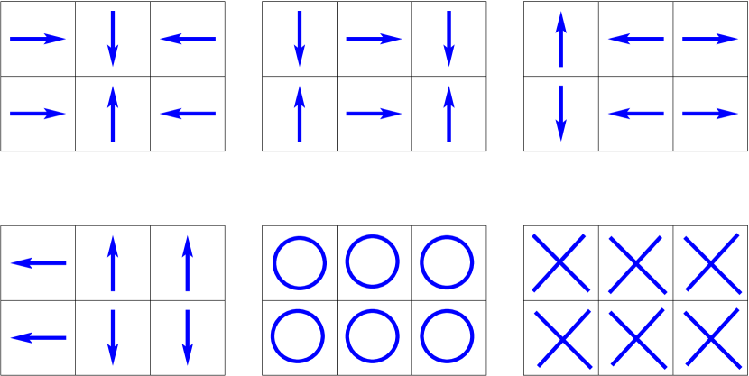
Figure 1.— A sequence of directional updates for the $3\times 2\times 1$ volume decomposition.

To summarize, in the hierarchy of events on a base grid every single hydrodynamical step is followed by a series of radiation-chemistry updates each of which in turn contains directional subcycling with flux exchanges among individual processors. When a spatial region is refined, radiation fluxes for both stellar and quasar components in all six directions are passed from parent grids to subgrids, along with all hydrodynamical variables.

2.3. Stage two: high angular resolution transfer

Our radiation hydrodynamics (RHD) calculation is parallelized via domain decomposition, in which we pass radiative intensities from one processor to another on the base grid, and in turn on each processor we advect these intensities along the AMR grid hierarchy. This approach results in a fairly complex algorithm, forcing us to limit RHD transport only to the six directions along the major axes. The total number of photons entering the volume in plane-parallel fluxes is kept the same as if we had an isotropic incident distribution, therefore those photons which burn their way into a denser environment at small solid angles tend to over-heat and over-ionize the medium. At the same time this approximation naturally leads to formation of shadows behind self-shielded regions which in reality could be exposed to ionizing radiation. To compensate for this shortcoming, we post-process our 3D ionization and temperature distributions with a much higher angular resolution radiative transfer code based on a new fully threaded transport engine algorithm (FTTE) by Razoumov & Cardall (2005).

At each output redshift we convert the block-structured AMR output of our coupled RHD runs to a fully threaded format and use it as a first guess to compute radiative transfer with FTTE along 192 directions chosen to subdivide the entire sphere into equal solid angle elements. We then use this updated radiation field to compute the ionizational structure and temperature, and then iterate in radiative transfer and chemistry until we find the equilibrium positions of HI, HeI and HeII ionization fronts at a given redshift. We find that $\sim 20$ iterations are needed for convergence.

2.4. Adopted UVB and frequency dependence

Constraints on the UVB at high redshifts come from the Ly$\alpha$ forest studies. Scott et al. (2000) used the proximity effect in quasar absorption spectra to derive the UVB amplitude assuming that it has the same spectrum as individual quasars. Using Ly-alpha emission line redshifts, they get the value $J_{\nu}=1.4^{+1.1}_{-0.5}\times 10^{-21}{\rm\,erg}{\rm\,s}^{-1}{\rm\,cm}^{-2}{\rm\,Hz}^{-1}{\rm\,sr}^{-1}$ for $1.7<z<3.8$. On the other hand, with OIII and MgII redshifts they get a lower value $J_{\nu}=7.0^{+3.4}_{-4.4}\times 10^{-22}{\rm\,erg}{\rm\,s}^{-1}{\rm\,cm}^{-2}{\rm\,Hz}^{-1}{\rm\,sr}^{-1}$ for $1.7<z<3.8$, corresponding to HI photoionization rate $1.9^{+1.2}_{-1.0}\times 10^{-12}{\rm\,s}^{-1}$.

More recently, Tytler et al. (2004) and Jena et al. (2005) build a concordance model of the Ly$\alpha$ forest at $z=1.95$ using a series of hydrodynamical simulations with grid sizes up to $1024^{3}$ and box sizes up to 76.8 Mpc to reproduce the observed flux decrement from the low-density intergalactic medium (IGM) alone. Their UVB corresponds to an ionization rate per H i atom of $\Gamma_{912}=(1.44\pm 0.11)\times 10^{-12}{\rm\,s}^{-1}$, which is slightly higher than the earlier estimates, e.g., the prediction by Madau et al. (1999) with 61% from QSOs and 39% from stars. The redshift evolution of this concordance model can be found in Paschos & Norman (2005). A more recent study by Kirkman et al. (2005) extends this higher estimate of $\Gamma_{912}\sim 1.4\times 10^{-12}{\rm\,s}^{-1}$ to the redshift range $2.2<z<3.2$ translating into $J_{\nu}\sim 5\times 10^{-22}{\rm\,erg}{\rm\,s}^{-1}{\rm\,cm}^{-2}{\rm\,Hz}^{-1}{\rm\,sr}^{-1}$.

Figure 2.— Amplitude of the assumed fiducial UVB at $13.6{\rm\,eV}$ in standard units of $10^{-21}{\rm\,erg}{\rm\,s}^{-1}{\rm\,cm}^{-2}{\rm\,sr}^{-1}{\rm\,Hz}^{-1}$. Shown are the quasar (dashed line) component $I_{21,{\rm q}}$ and the stellar (dotted line) component $I_{21,*}$, and their sum (solid line) at the hydrogen Lyman edge for $\beta_{*}=\beta_{\rm q}=1$. For comparison we also plotted the total UVB from Abel & Haehnelt (1999) (dash-dotted line).

The background in the vicinity of DLAs in a cluster that does not host a quasar is most likely going to be smaller than these average values, due to the geometrical dilution factor, and local attenuation in the cluster. In our other models not listed in Table 1 we experimented with a variety of UVB spectra and amplitudes, and as a reference we decided to use a smaller background based on Abel & Haehnelt (1999). We included both stellar and quasar ionizing photons adopting a two-component power-law UVB

$$I_{\nu}=\beta_{*}I_{21,*}\left(\frac{\nu}{\nu_{L}}\right)^{-\alpha_{*}}+\beta_{\rm q}I_{21,{\rm q}}\left(\frac{\nu}{\nu_{L}}\right)^{-\alpha_{\rm q}}$$ (2)

where $\alpha_{*}=5$, $\alpha_{\rm q}=1.8$, and $\beta_{*}$ and $\beta_{\rm q}$ are the model parameters. We extend the stellar and quasar components of Abel & Haehnelt (1999) to higher redshifts with the expressions

$$I_{21,{\rm q}} = Q+a(S-Q),$$ (3)

$$I_{21,*} = \left(S+a(Q-S)\right)\left(1-\tanh(0.5z-7)\right)/2,$$

where

$$Q = {10\exp[-(z/2.5)^{3}]\over 1+(7/(1+z))^{4}},$$ (4)

$$S = {1-b\over 2}{\exp[-(z/4)^{3}]\over 1+(7/(1+z))^{4}}+$$

$${b~{}(1+z)^{3.35}\over 106.4}\exp\left[-(z-0.5)^{2}\over 1+(z+2.09)^{2.075}/16\right],$$

$$a = 0.3\exp[-(z-4.5)^{2}/4],$$

$$b = 1+\tanh(1.5z-6.3).$$

We plotted $I_{21,*}$, $I_{21,{\rm q}}$ and the background from Abel & Haehnelt (1999) in Fig. 2. We allow for a substantial stellar component at $z>8$, which is consistent with the current theoretical views of the global history of SF in a $\Lambda$CDM Universe (Springel & Hernquist, 2003) in light of the discovery of a large optical depth to electron scattering by WMAP (Kogut et al., 2003) suggesting presence of bright ionizing sources at $z\sim 15-17$ (Wyithe & Loeb, 2003; Haiman & Holder, 2003; Hui & Haiman, 2003; Ciardi et al., 2003). As the main focus of this paper is to study the resolution effects of radiative transfer in galaxy formation models, we do not explore other possible star formation histories, but undoubtedly the cumulative history of star formation at $z>6$ might have an important effect on the observable properties of galaxies even at lower redshifts.

We use three frequency bands, $13.6-24.6{\rm\,eV}$, $24.6-54.4{\rm\,eV}$, and above $54.4{\rm\,eV}$, to compute H i , He i and He ii ionization. Inside each frequency band $[{\nu_{\rm g}},{\nu_{{\rm g}+1}}]$ the transport variable is the intensity at frequency ${\nu_{\rm g}}$ weighted by a corresponding power-index-dependent factor

$$f_{\rm g}={1-\left({\nu_{{\rm g}+1}}/{\nu_{\rm g}}\right)^{1-{\alpha_{\rm g}}}\over{\alpha_{\rm g}}-1},$$ (5)

where ${\rm g}=1,2,3$. All radiation-related rates (photoionization, photoheating, and absorption) also depend on ${\alpha_{\rm g}}$. Finally, inside each frequency band we use a single transport variable describing both stellar and quasar components with an effective index ${\alpha_{\rm g}}$ constructed to ensure that the total energy inside the band is equal to the sum of the two individual components.

2.5. Spectrum generation

To analyze the statistical properties of DLAs, we drew 100,000 random (through a random point in a random direction) lines of sight through the entire grid hierarchy of each model using the highest resolution cells available at each point along the line, and studied all absorption systems with HI column densities ${N_{\rm HI}}\geq 2\times 10^{20}{\rm\,cm}^{-2}$. For analysis we use two “low ion” lines of Si II at $1526{A}$ and $1808{A}$. Since the latter line has a significantly lower oscillator strength, we use it only in absorbers with $\log({N_{\rm HI}}/{\rm\,cm}^{-2})>20.6$, and for the lower column densities use the former transition. We assume a uniform abundance throughout the volume with metallicity $[{\rm Si/H}]=-1.3$ (Wolfe et al., 2005). Noise is added to our artifical spectra such that the resultant signal-to-noise ratio of each $1{\rm\,km\,s^{-1}}$ pixel is 20:1. We define the Si II line width as the width of the central part of the profile responsible for $90\%$ of the integrated optical depth as described in Prochaska & Wolfe (1997). In the unlikely case that a line of sight crosses multiple absorbers, we consider two components to be caused by a single DLA if the separation between the centers of the two corresponding line profiles is less than $400{\rm\,km\,s^{-1}}$, otherwise we just analyze the strongest component.

3. Results

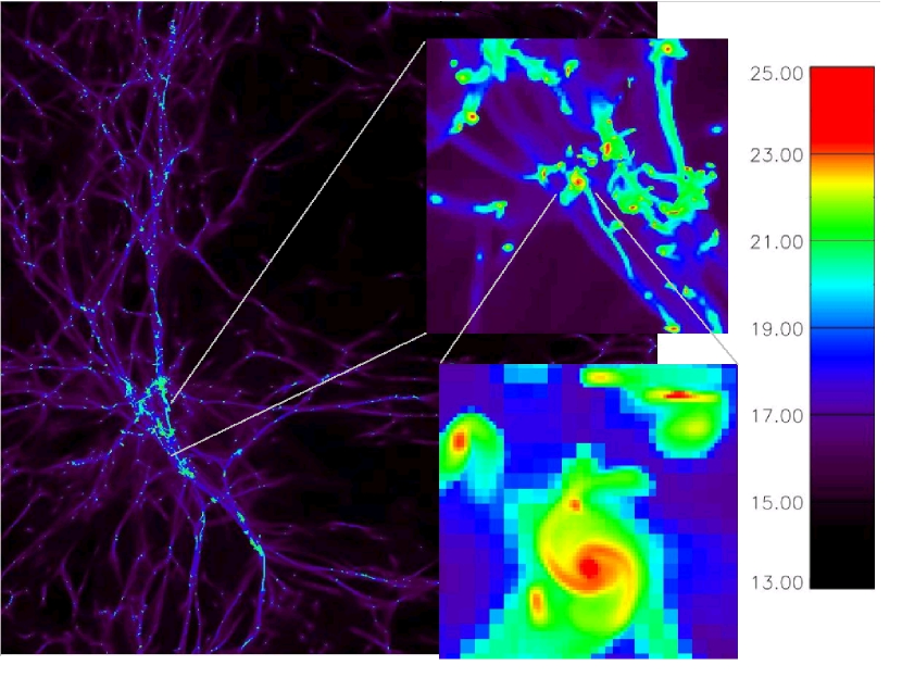
Figure 3.— HI column density in a volume $8h^{-1}{\rm\,Mpc}$ on a side and $8h^{-1}{\rm\,Mpc}$ thick (comoving), from run C1 at $z=3$. The zoom-in boxes are $600h^{-1}{\rm\,kpc}$ (top) and $80h^{-1}{\rm\,kpc}$ (bottom) on a side in comoving units, translating into an approximately $10{\rm\,kpc}$ (physical units) DLA around the disk galaxy in the center of the bottom panel. The DLA column densities correspond to green and up in the color map on the right. The resolved dynamic range in this model is 8192.

To demonstrate the nature of DLAs produced in our models, in Fig. 3 we plotted the projected HI column density in a volume 8 Mpc on a side and 8 Mpc thick, for run C1 at $z=3$, with zoom-ins on a cluster of galaxies and a disk galaxy. All objects with HI column densities above $2\times 10^{20}{\rm\,cm}^{-2}$ give rise to DLAs. To investigate the validity of our results and compare them to observations, we use two types of distributions: the HI column density frequency distribution $f(N,X)$ and the line density $\ell_{\rm DLA}(X)$ of DLAs with the Si II velocity width higher than $v_{\rm SiII}$ vs. $v_{\rm SiII}$. The frequency distribution $f(N,X)$ is defined such that $f(N,X)dNdX$ is simply the number of DLAs in the intervals $[N,N+dN]$ and $[X,X+dX]$, where $dX$ is the “absorption distance” interval

$$dX={H_{0}\over H(z)}(1+z)^{2}dz.$$ (6)

In principle, any combination of the following four factors can affect our results: finite grid resolution, finite mass resolution, the amplitude and spectrum of the assumed UV background, and radiative and mechanical feedback from SF. As the goal of this work is to demonstrate a method to compute the ionization structure of the outskirts of high redshift galaxies with self-consistent radiative transfer of the UVB, we do not include the uncertainties of feedback from SF here. In this paper we concentrate on resolution issues in the new models and the dependency on the UVB, at a fixed redshift ($z=3$). In our next paper we will study the redshift evolution and stellar feedback.

3.1. Numerical resolution

In Fig. 4 we plotted $f(N,X)$ for all of our runs at $z=3$. For comparison, we also plotted the data from the SDSS DLA survey from Prochaska et al. (2005) for redshift intervals $z=2.5-3.0$ and $z=3.0-3.5$. The top panel shows our $8h^{-1}{\rm\,Mpc}$ models, for which the grid resolution ranges from $4h^{-1}{\rm\,kpc}$ (comoving) for run C-1 to $0.5h^{-1}{\rm\,kpc}$ for run C2. At this redshift these numbers translate into 1.5 kpc and 190 pc physical resolution, respectively. Although the results have not converged yet at our highest resolution, the trend is clear: as we increase grid resolution, the baryons in halos can collapse further yielding smaller DLA cross-sections. For any curve, the disagreement between models and observations is the largest for high-column density systems which have the sharpest baryon concentrations and are particularly sensitive to grid resolution.

The challenging aspect of the DLA modeling is clearly illustrated in the lower panel in Fig. 4 in which we apply the same $128^{3}$ base grid with 6 levels of refinement to a smaller ($4h^{-1}{\rm\,Mpc}$) volume, resulting in two times better grid resolution and eight times higher mass resolution (run B1, dashed line). Unlike model C1 (solid line), this run has a population of self-shielded halos in the $10^{8}-10^{9}{\rm\,M_{\odot}}$ mass range. While naively one would expect to see higher $f(N,X)$, especially at low column densities, this effect is almost precisely offset by the reduced size of individual halos through higher grid resolution. This is further seen in run A1 (dotted line), which extends the population of self-shielded halos down to $\sim 7\times 10^{7}{\rm\,M_{\odot}}$ but features almost identical $f(N,X)$.

Figure 4.— Top panel: the upper four solid lines show the HI column density frequency distribution $f(N,X)$ for runs C-1 , C0, C1, and C2 (from thin to thickest line), all at $z=3$. The lower two lines are the $\Gamma$-function fits to the SDSS DLA survey data from Prochaska et al. (2005) for $z=2.5-3.0$ (dashed) and $z=3.0-3.5$ (dotted). Lower panel: same as in the top panel, except that the upper three lines give $f(N,X)$ for runs C1 (solid), B1 (dashed), and A1 (dotted).

The same effects can be observed in Fig. 5 which shows the line density $\ell_{\rm DLA}(X)$ of DLAs per unit absorption distance with the Si II velocity width higher than $v_{\rm SiII}$. This figure is similar to the cumulative abundance plots vs. halo circular velocity (or mass) in Gardner et al. (2001) and Nagamine et al. (2004), but we chose the neutral gas line width as a more generic measure of the strength of the absorber, since our simulated absorbers can also be caused by tidal tails and filaments. The horizontal lines in Fig. 5 show the mean observed DLA line density from Prochaska et al. (2005).

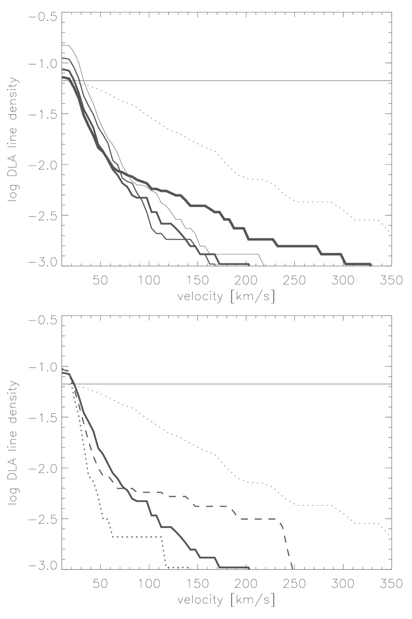
Figure 5.— Top panel: line density $\ell_{\rm DLA}(X)$ of DLAs with the Si II velocity width higher than $v_{\rm SiII}$ vs. $v_{\rm SiII}$, at $z=3$. The lines correspond to models C-1 , C0, C1, and C2 (from thin to thickest line). The dotted line shows the observed kinematic distribution from data at all redshifts, compiled from Fig. 10 in Wolfe et al. (2005) and normalized to match the cumulative observed value $0.067\pm 0.006$ at $z=3$ (horizontal line). Lower panel: same as in the top panel, except that the three thick lines give $\ell_{\rm DLA}(X)$ for runs C1 (solid), B1 (dashed), and A1 (dotted).

In the top panel we see a monotonic decrease in the line density of DLAs as we increase the grid resolution. The higher velocity tail is not affected until we compute our highest resolution model C2 which starts to resolve individual minihalos in the highest density regions. With a certain probability that is related to the physical size of their neutral cores, these small galaxies (with a few tidal streams mixed in) can be seen as multiple absorption components in a single line of sight to a remote quasar.

This effect can be further illustrated in Fig. 6 in which we plotted Si II $1526{A}$ or $1808{A}$ line profiles for a typical DLA (top profile) and for nine DLAs with largest velocity widths (profiles 2-10, from top to bottom) in model C2. With the line detection criteria defined in Sec. 2.5, we found the following velocity widths for these spectra: 31, 468, 191, 149, 281, 168, 170, 306, 193, and 205 ${\rm\,km\,s^{-1}}$ (from top to bottom panels in Fig. 6). Spectra 2 and 8 (counting from the top) are particularly clear examples of several components falling onto the same line of sight. These multiple component DLAs give rise to distinct tails at higher velocities which stand out in our high (190 pc physical) resolution models C2 (upper panel) and B1 (lower panel). While the highest resolution run A1 (lower panel) shows a similar tail, it is shifted towards lower ($65-100{\rm\,km\,s^{-1}}$) velocity widths, in part due to the smaller velocity dispersion in the cluster, and in part due to the lower cross-sections of individual absorbers.

Figure 6.— Si II $1526{A}$ (or $1808{A}$) line profiles for ten selected DLAs in run C2 at $z=3$.

To summarize, none of our models at this stage are able to reproduce the observed velocity width distribution for systems with $v_{\rm SiII}~{}\raise 1.29167pt\hbox{$>$}\kern-7.5pt{\lower 2.79857pt\hbox{$\sim$}}~{}30{\rm\,km\,s^{-1}}$. Although the resolution effects are complex, and none of our models have fully converged to the observed column density distribution yet, it seems plausible that some of the effects described in this section can drive the line profile distribution to even lower velocities. For example, as we increase grid resolution, fewer and fewer systems will be crossed by the same line of sight, moving many DLAs in Fig. 5 from $100-400{\rm\,km\,s^{-1}}$ into the $30-100{\rm\,km\,s^{-1}}$ range. We therefore conclude that feedback from star formation seems to be the most likely mechanism to get DLA velocity widths as high as indicated by observations. In our future simulations, in addition to exploring feedback, we will also strive to increase mass resolution in progressively larger simulation volumes, which should produce many more self-shielded halos with masses of few $10^{8}{\rm\,M_{\odot}}$ in galaxy clusters with larger velocity dispersions.

3.2. Halo and intergalactic DLAs

We find that the nature of DLA absorption is a function of the halo environment. The cumulative halo mass function in our $8h^{-1}$, $4h^{-1}$ and $2h^{-1}{\rm\,Mpc}$ volumes at $z=3$ is plotted in Fig. 7. Most of these halos give rise to DLAs; however, not all DLAs can be associated with individual halos.

Figure 7.— Cumulative halo mass function at $z=3$ for dark matter only, for runs C1 (thick solid line), B1 (thick dashed line), and A1 (thick dotted line). The thin solid line is the analytical mass function from Mo & White (2002).

Gardner et al. (1997) assumed a relation between the neutral hydrogen cross-section and the host halo mass to predict the total abundance of DLAs in a large simulation volume. On the other hand, Nagamine et al. (2004) computed this relation for individual halos in a series of SPH models with the assumption that all DLAs are fully neutral and therefore a self-shielding correction is not necessary.

Since we include the effects of the UVB on gas at the surface of DLAs, it is interesting to make an independent estimate of neutral hydrogen cross-sections for individual absorbers in our models. We draw a large number ($N_{\rm LOS}=10^{8}$) of random lines of sight parallel to all three major axes, and find all absorption systems with the neutral hydrogen column density above $2\times 10^{20}{\rm\,cm}^{-2}$. We then look for all halos inside the same base grid cell as the geometrical center of a DLA, find the one which is closest to this DLA, and associate it with this absorption system. Some extended DLAs caused by intergalactic HI will have no host halos. Halos were identified with the HOP algorithm (Eisenstein & Hut, 1998) using the routine enzohop which is part of the Enzo package. Following this procedure, we count the number of damped systems $N_{\rm DLA}$ associated with each halo. Then the effective radius of the absorber can be estimated approximately as

$$r_{\rm eff}=\sigma^{1/2}\approx L_{\rm box}\left(N_{\rm DLA}\over N_{\rm LOS}\right)^{1/2},$$ (7)

where $L_{\rm box}$ is the physical box size. In Fig. 8 we plotted a relation between the halo mass $M_{\rm halo}$ and its absorption radius $r_{\rm eff}$ in runs A1 (diamonds), B1 (triangles), and C2 (crosses). A least-squares fit to these data with equation

$$\log(r_{\rm eff}/{\rm\,kpc})=\alpha\log(M_{\rm halo}/{\rm\,M_{\odot}})+\beta$$ (8)

gives $\alpha=0.38$ and $\beta=-3.07$ (thick solid line). At $z=3$ our absorption cross-sections are approximately a factor of two lower than the ones in Nagamine et al. (2004). To avoid any confusion, we want to stress that this finding does not contradict our DLA counts in Fig. 4 and 5 since the halos in Fig. 8 do not represent all DLAs in the volume as this plot does not include intergalactic HI clouds. In addition, our data in Fig. 8 should be viewed as lower limits to DLA cross-sections rather than their actual values since in a massive cluster environment very often we cannot identify a single halo responsible for a particular DLA. For example, in Fig. 3 we can see larger HI clouds engulfing multiple halos. For this reason, in our estimate of $r_{\rm eff}$ we only searched for halos inside the same base grid cell as the geometrical center of a DLA which undoubtedly underestimates the true absorption cross-section.

In addition, interactions between galaxies in more massive environments create tidal streams which can produce DLA lines. The cluster in our $8h^{-1}{\rm\,Mpc}$ volume at $z=3$ has extended HI tails formed by galaxy-galaxy interactions which – at certain line of sight orientations – produce column densities in the range $2\times 10^{20}-5\times 10^{21}{\rm\,cm}^{-2}$. The typical physical density in the self-shielded filaments in these streams is of order $\sim 10^{-2}{\rm\,cm}^{-3}$, the hydrogen neutral fraction often (but not always) exceeds $0.9$, and physical widths are of order $5-10{\rm\,kpc}$. Gas which is not self-shielded from the UVB will never reach these column densities, unless perhaps it is highly compressed into shocks by feedback which we do not include here.

To estimate the fraction of the line density $\ell_{\rm DLA}(X)$ due to gas outside of halos, we removed all neutral hydrogen from inside the virial radii of all halos in the highest resolution $8h^{-1}$ run C2, and reran the analysis. We defined the virial radius as the radius of the sphere that encloses 180 times the mean mass density of the Universe at that redshift. We found that at our highest numerical resolution approximately 29% of all DLAs are due to gas outside of galaxies at $z=3$. While in the original run C2 the highest DLA column density is $10^{23.8}{\rm\,cm}^{-2}$, it changes to $10^{21.5}{\rm\,cm}^{-2}$ if we consider only intergalactic gas.

On the other hand, in less massive halo environments, especially in the smaller $4h^{-1}$ and $2h^{-1}{\rm\,Mpc}$ simulation volumes, the main reason behind our fairly large DLA counts despite the small effective cross-sections is a much larger contribution to $f(N,X)$ from lower mass halos in the range $\sim 7\times 10^{7}-10^{8}{\rm\,M_{\odot}}$ which we demonstrate below.

Figure 8.— Effective radius vs. halo mass, for all DLAs with identified host halos in runs A1 (diamonds), B1 (triangles), and C2 (crosses) at $z=3$, for the fiducial background in Fig. 2. This figure does not account for DLAs caused by intergalactic HI clouds for which no host halo in the same base grid cell was found. The dotted horizontal line shows the size of the base grid cell in the $8h^{-1}{\rm\,Mpc}$ volume. The solid lines are our least-squares fits with eq. 8 for all halos from runs A1, B1 and C2 (thick line), and all halos from runs A1, B1 and C1 (thin line). For comparison, we also plotted the fits to DLA radii from Nagamine et al. (2004), for models O3 (dashed line, no wind, 10 Mpc volume), Q3 (dashed-dotted line, strong wind, 10 Mpc volume, low resolution) and Q5 (dotted line, strong wind, 10 Mpc volume, high resolution).

3.3. Photoionization of low-mass galaxies

It is well known that low-mass galaxies cannot retain gas after reionization. The exact value of the cut-off is not very well established and without doubt depends on the local environment. Nagamine et al. (2004) notice a sharp drop-off in the DLA cross-section below the mass $\sim 10^{8}M_{\odot}$ which they associate with photoevaporation of gas in these halos by the ionizing UVB and/or with supernovae feedback.

Among all of our models, the least massive halo which is associated with a DLA has a dark matter mass $3.6\times 10^{7}{\rm\,M_{\odot}}$ (Fig. 8). It was found in run A1 in which the halo mass function extends down to $1.4\times 10^{7}{\rm\,M_{\odot}}$ (Fig. 7) which is $\sim 35$ times the mass resolution of this run. The two other least massive halos associated with DLAs were also found in this highest resolution run. However, it is only above the mass $\sim 7\times 10^{7}{\rm\,M_{\odot}}$ that we start seeing a significant population of halos with HI in absorption.

The fact that we see neutral gas in halos with masses slightly below the cut-off of Nagamine et al. (2004) can be attributed to both the spatial variations in the UVB inside the galaxy cluster and the lack of supernova feedback in our models. As Nagamine et al. (2004) pointed out, a sharp cut-off should be expected due to the strong dependence of baryon cooling and photoheating on the virial temperatures of halos around $\sim 10^{4}{\rm K}$. In fact, we see such a cutoff at $\sim 7\times 10^{7}{\rm\,M_{\odot}}$ in Fig. 8. As all photoionizing radiation in our models comes from the box boundary, few low-mass halos might be shadowed by other more massive systems and be able to retain their neutral gas, as we see in two or three galaxies with masses below $7\times 10^{7}{\rm\,M_{\odot}}$. Furthermore, a number of galaxies in the mass range $7\times 10^{7}{\rm\,M_{\odot}}-10^{8}{\rm\,M_{\odot}}$ are not exposed to the full UVB as part of their “sky” is blocked by nearby absorption systems (see, e.g., the zoom-in panels in Fig. 3), and the mass cut-off above which galaxies can retain neutral gas is shifted towards slightly lower masses. Of course, this effect depends on the environment and will be more pronounced at higher redshifts where the spatial variations in the UVB are larger. Star formation and supernova feedback will partially reverse this effect removing neutral material from lower mass galaxies assuming that these galaxies have accumulated enough cold gas to host star formation in the first place. However, this effect is very complex and, in addition to the mechanical feedback from winds and supernovae, will have to include transfer of locally generated UV photons.

3.4. Dependence on the UVB

Our distributions are somewhat sensitive to a change in the UVB. In model C1 we varied the quasar component from the fiducial value in Fig. 2 to twice (C1b) and four times (C1c) that amplitude and plotted the results in Fig. 9. As we increase the UVB amplitude and simultaneously steepen its spectrum, more HI is ionized everywhere on the outskirts of galaxies, but in terms of DLA statistics – not surprisingly – primarily low column density systems are affected. While the under-resolved model C1 features the cumulative number of DLAs $\sim 25\%$ above the observed value at $z=3$, the higher UVB model C1c has the number of DLAs $\sim 25\%$ below the observed value. Noticeable differences between the two models extend to the column density $10^{21.4}{\rm\,cm}^{-2}$, but the higher column density systems are not affected.

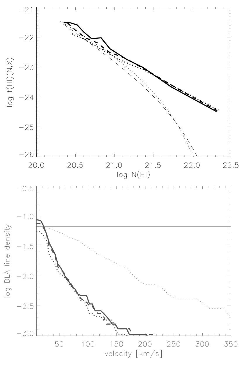
Figure 9.— The three thick lines in each panel show results for a run with the full quasar background from Fig. 2 (C1, solid line), and runs with two times (C1b, dashed line) and four times (C1c, dotted line) the fiducial quasar background, all at $z=3$. Top panel: HI column density frequency distribution $f(N,X)$. The two thin lines are the SDSS DLA survey data as in Fig. 4. Lower panel: line density $\ell_{\rm DLA}(X)$ of DLAs with the Si II velocity width higher than $v_{\rm SiII}$ vs. $v_{\rm SiII}$. The thin dotted and thin horizontal lines show the observed kinematic distribution as in Fig. 5.

3.5. Effects of radiative transfer

In addition to the full radiative transfer run C2 in the $8h^{-1}{\rm\,Mpc}$ volume, we also computed a model C2s with complete self-shielding above the physical density $10^{-2}{\rm\,cm}^{-3}$, assuming that the local UVB is just the uniform cosmic background from Fig. 2 in every cell below this threshold, and zero above it. This assumption has been previously used in DLA modeling, e.g., in Haehnelt et al. (1998). We also computed a model C2t with the optically thin approximation imposing the same uniform cosmic UVB in every cell in the volume. In Fig. 10 we plotted distributions for these three models. All three models were iterated until H/He ionization equilibrium.

It is evident that self-shielding of neutral gas is the dominant mechanism determining all properties of DLAs. The model with the uniform background in the optically thin regime produces very few DLAs as expected. Surprisingly, the full transfer model and the one with self-shielding give roughly the same cumulative number of DLAs. However, since the transfer model includes high energy photons, the ionizational structure of HI regions is more complex than in the fully shielded case. These differences result in vastly different line widths distributions: in the self-shielded model most lines widths are clustered around $15{\rm\,km}{\rm\,s}^{-1}$, whereas in the model with transfer they are concentrated at higher velocities in the range $15-30{\rm\,km\,s^{-1}}$. It is reassuring that the model with full transfer in the lower panel in Fig. 10 is about half-way from the self-shielded model to observational data.

It is important to point out that our self-shielded model produces results very different from Haehnelt et al. (1998), namely substantially smaller velocity widths on average. A number of factors could contribute to this difference, such as the use of Eulerian hydrodynamics with AMR instead of SPH, but perhaps the most important factors are our much larger sample of galaxies (we used 710 distinct halos to generate 406 DLAs in runC2s vs. their sample of 40 protogalactic clumps used repeatedly to produce 640 DLAs), and our much higher grid resolution (190 pc physical vs. their 1 kpc). But as we point out, our full radiative transfer runs produce further improvement in kinematics modeling rendering any self-shielded models obsolete.

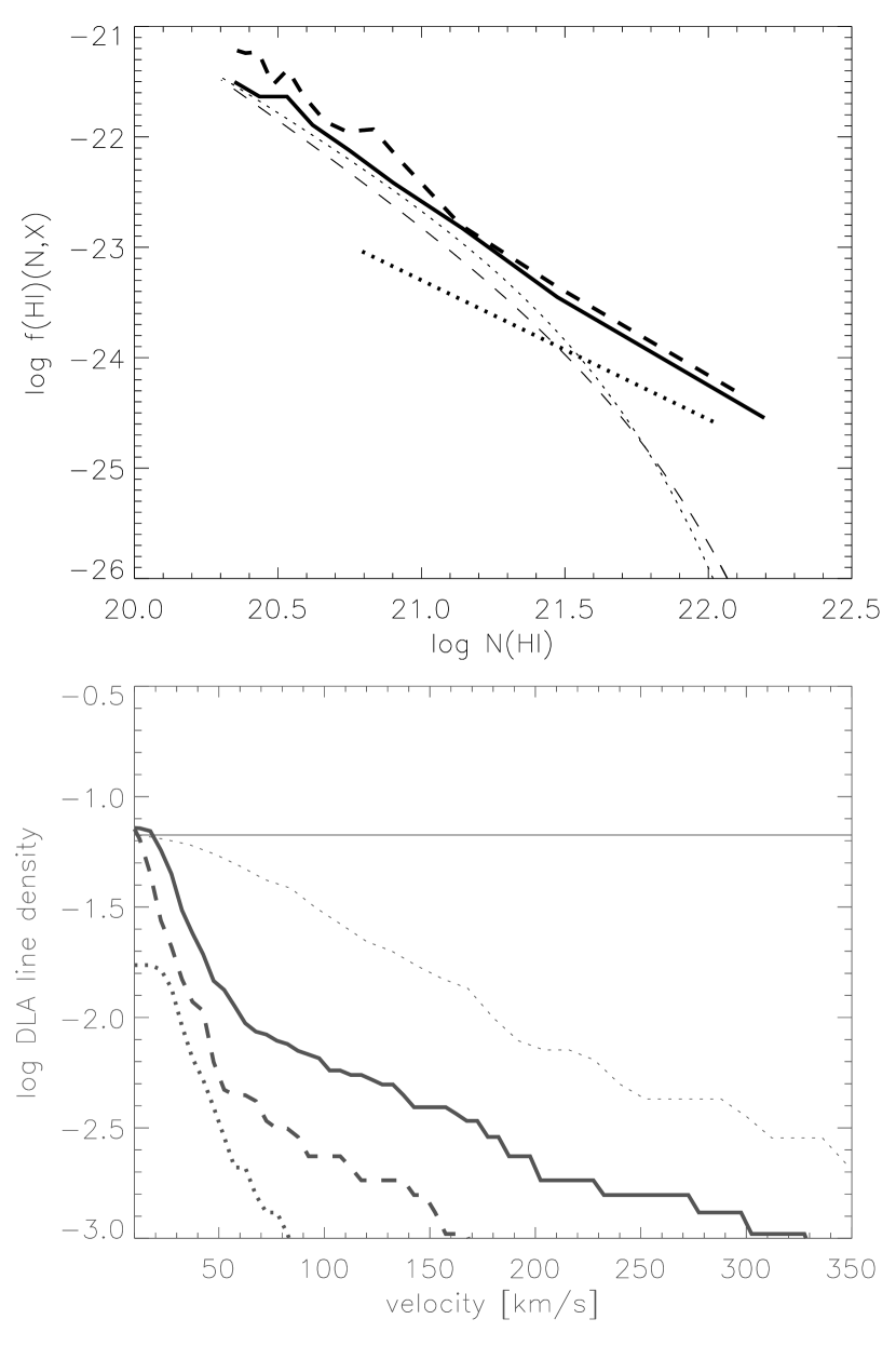
Figure 10.— The three thick lines in each panel show results for a run with full radiative transfer (C2, solid line), a run with self-shielding above the physical density $10^{-2}{\rm\,cm}^{-3}$ (C2s, dashed line), and a run with the optically thin approximation throughout the entire simulation volume (C2t, dotted line), all at $z=3$. Top panel: HI column density frequency distribution $f(N,X)$. The two thin lines are the SDSS DLA survey data as in Fig. 4. Lower panel: line density $\ell_{\rm DLA}(X)$ of DLAs with the Si II velocity width higher than $v_{\rm SiII}$ vs. $v_{\rm SiII}$. The thin dotted and thin horizontal lines show the observed kinematic distribution as in Fig. 5.

In Fig. 11 we plotted the mean specific intensity at $13.6{\rm\,eV}$, $24.6{\rm\,eV}$ and $54.4{\rm\,eV}$ vs. the local gas number density at $z=3$. One can easily see hardening of the spectrum in self-shielded regions above the physical density $10^{-2}{\rm\,cm}^{-3}$, as more energetic photons travel further in the neutral medium.

Figure 11.— Mean specific intensity (${\rm\,erg}{\rm\,s}^{-1}{\rm\,cm}^{-2}{\rm\,Hz}^{-1}{\rm\,sr}^{-1}$) vs. gas number density in model C1 at $z=3$ at photon energies $13.6{\rm\,eV}$ (solid line), $24.6{\rm\,eV}$ (dashed line) and $54.4{\rm\,eV}$ (dotted line).

4. Summary

The standard hierarchical model is very successful in explaining the emergence of structures in the early Universe. DLAs are viewed as neutral gas clouds confined to individual galaxies, whether in virialized systems or systems still in the process of merging. This paradigm is clearly seen in most previous DLA simulation literature where analysis is based on a fit to the relation between DLA cross-section and halo mass. The results of high resolution simulations by Haehnelt et al. (1998) suggest that small protogalactic clumps in the process of merger could explain the observed line profiles, and the statistical analysis of absorption line kinematics within semi-analytical models by Maller et al. (2001) suggests that tidal tails can be responsible for absorption.

To test both these hypotheses and a broader idea that DLAs can be caused by absorption in neutral intergalactic clouds either stripped of galaxies during interactions or even still accreting onto galaxies from the IGM, we propose to include radiative transfer of the UVB into galaxy formation models, and argue that this new piece of physics is essential in order to reproduce DLA observables such as the column density and velocity width distributions. An accurate treatment of background photons allows us to address the ionization structure of the outskirts of high redshift galaxies in a much more precise way.

We simulate galaxy formation in a series of cosmological volumes ranging in size from 2 Mpc to 8 Mpc, solving simultaneously for the first time coupled equations of hydrodynamics, self-gravity, multi-species chemistry and radiative transfer to account for shielding against the UVB. Radiative transfer is computed on all levels of grid refinement with a two-stage calculation, first just along the three major axes simultaneously with hydrodynamics, and then in 192 directions in the postprocessing mode. We use AMR to resolve individual galaxies with the same refinement criteria everywhere in the volume. Similar to Nagamine et al. (2004), we use a series of computational volumes of different sizes while varying numerical resolution to try to achieve optimal balance between resolution and fair volume sampling. However, because we do not restrict damped Ly$\alpha$ absorption to halos, we do not assume any single relation between DLA cross section and halo mass for analysis. There is a relation between DLA cross-section and associated line width which in some cases is indeed caused by the velocity dispersion within individual galaxies. Our findings are as follows.

• Resolution: As we increase grid resolution, our column densities demonstrate a trend in convergence towards the observed distributions. However, we cannot reproduce the high-end tail of the velocity width distribution. Although it is possible that the resolution effects and limitation in box sizes are responsible for this shortcoming, feedback from star formation which we have not included into the current models is likely to produce expanding shells and therefore higher velocity widths on average. The column density distributions alone indicate that the minimum required grid resolution has to be better than $\sim 500{\rm\,pc}$ in comoving coordinates, or $\sim 100{\rm\,pc}$ in physical space. The minimum mass resolution is $\sim 10^{6}{\rm\,M_{\odot}}$ corresponding to at least a hundred DM particles per halo which is still capable of being self-shielded from the UVB.

• Filamentary DLAs: The nature of DLA absorption is a function of halo environment, at any given redshift. Although all self-shielded halos can give rise to DLAs, not all DLAs can be associated with individual halos. We find that in massive cluster environments at $z=3$ tidal tails and quasi-filamentary structures often appear to be self-shielded against the UVB. The typical column densities of filamentary DLAs are below $10^{21}{\rm\,cm}^{-2}$, and physical widths are of order $5-10{\rm\,kpc}$. Since we have not achieved numerical convergence, we have not attempted a comprehensive, redshift-dependent statistical study to distinguish halo DLAs from the ones caused by tidal tails, and both of these from DLAs caused by primordial gas still accreting onto galaxies.

  Provided that filamentary structures are still self-shielded at higher grid resolution, it seems plausible that going to higher resolution would only increase the filamentary contribution to DLA absorption, as the 3D density peaks (halos) would contribute progressively less to the total HI column density than the 2D density peaks (filaments) as baryons cool and collapse on finer grids.

• Photoionization of low-mass galaxies: The least massive single galaxy associated with DLAs in our models has the mass $3.6\times 10^{7}{\rm\,M_{\odot}}$. However, we see a significant population of halos with HI in absorption only above the mass $\sim 7\times 10^{7}{\rm\,M_{\odot}}$ below which just a few dwarf galaxies retained any sufficient amount of neutral gas by $z=3$. This threshold is slightly lower than the previously reported values of $10^{8}{\rm\,M_{\odot}}$ to few $10^{8}{\rm\,M_{\odot}}$ (Nagamine et al., 2004) contributing to larger DLA counts in less massive halo environments. Part of this discrepancy can be explained by spatial variations in the UVB inside the galaxy cluster, and it is possible that supernova feedback which is not included into our models could also have a role removing neutral gas from low-mass galaxies.

• Self-shielding model: Calculations with self-shielding above density $10^{-2}{\rm\,cm}^{-3}$ produce roughly the same total number of DLAs per unit absorption distance as the run with full radiative transfer. However, the absorption line width distributions in the two models are markedly different due to variations in ionizational profiles.

We intend this work to be the first in a series of papers exploring DLA properties with our new cosmological simulations with high-angular resolution radiative transfer on adaptively refined meshes. A number of topics are open to further exploration.

1) At the moment it is not clear to what extent DLAs produced with full coupled RHD simulations of galaxy formation would be different from the ones we get with our radiative-chemical postprocessing approach. Inclusion of radiative terms into hydrodynamical equations might be important for both accessing the effect of the external UV irradiation of primordial galaxies (Iliev et al., 2005) and studying feedback from SF (Whalen et al., 2004; O’Shea et al., 2005).

2) We have not included SF into our current models. Its mechanical and radiative feedback could change the ionization structure and kinematics of gas in high-redshift galaxies. For example, winds from SF regions and/or SNe could create denser shells around low-density bubbles. If dense enough, these shells might contribute to an overall increase in DLA effective cross-sections (Schaye, 2001). Of course, there is a competing effect if feedback destroys neutral gas in halos as observed in Nagamine et al. (2004).

3) Besides an obvious merit of providing more statistics, going to larger simulation volumes of few tens ${\rm\,Mpc}$ would allow us to test the effect of large-scale fluctuations in the UVB on absorption properties of high-redshift galaxies. The average separation between quasars at $z=3-4$ is more than an order of magnitude greater than our current largest simulation volume. Similar to the proximity effect observed in quasar spectra, very few halos would produce a DLA in a cluster that hosts a quasar. As we move further away from a quasar, the mean background drops. It is also attenuated in large clusters of galaxies due to the overall higher IGM column densities. If the typical UVB in the vicinity of DLAs is 50-75% lower than the cosmic average, it could yield dramatically different DLA counts. In addition, larger simulation volumes would produce more massive clusters of galaxies, with more violent interactions and more prominent tidal tails which would also have a direct impact on DLA observables.

4) To restrict our parameter space, we omitted an interesting topic of fine-tuning the initial power spectrum (particularly on galactic scales) to match the observed line density of DLAs which we are planning to do in the future.

In order to derive a single realistic population of hydrogen absorbers from Ly$\alpha$ forest clouds to DLAs, ideally one would like to build a sub-kpc resolution model with both stellar feedback and UVB radiative transfer in a large (50-80 Mpc) volume. To achieve the required mass and grid resolution, one would need to use grids of sizes 2048L6 with $2048^{3}$ DM particles. An N-body model of this size (but in a much larger volume) has been recently computed by the Virgo Consortium – the “Millennium Simulation” (Springel et al., 2005) – and can be potentially postprocessed with our fully threaded transport engine following the routine utilized in this paper.

5. Acknowledgments

This work was supported by Scientific Discovery Through Advanced Computing (SciDAC), a program of the Office of Science of the U.S. Department of Energy (DoE); and by Oak Ridge National Laboratory, managed by UT-Battelle, LLC, for the DoE under contract DE-AC05-00OR22725. At the beginning of this project AOR was partially supported by NSF grants AST-9803137 and AST-0307690. JXP and AMW are partially supported by NSF grant AST-03-07824. Numerical simulations were performed using the IBM DataStar system at the San Diego Supercomputer Center.

References

- Abel et al. (1997) Abel, T., Anninos, P., Zhang, Y., & Norman, M. L. 1997, New Astronomy, 2, 181
- Abel & Haehnelt (1999) Abel, T. & Haehnelt, M. G. 1999, ApJ, 520, L13
- Anninos et al. (1997) Anninos, P., Zhang, Y., Abel, T., & Norman, M. L. 1997, New Astronomy, 2, 209
- Bryan & Norman (1999) Bryan, G. L. & Norman, M. L. 1999, in IMA, Vol. 117, Adaptive Mesh Refinement (SAMR) Grid Methods, ed. S. B. Baden, N. P. Chrisochoides, D. Gannon, & M. L. Norman, New York: Springer, 165
- Ciardi et al. (2003) Ciardi, B., Ferrara, A., & White, S. D. M. 2003, MNRAS, 344, L7
- Colella & Woodward (1984) Colella, P. & Woodward, P. R. 1984, J. Comp. Phys., 54, 174
- Eisenstein & Hut (1998) Eisenstein, D. J. & Hut, P. 1998, ApJ, 498, 137
- Gardner et al. (1997) Gardner, J. P., Katz, N., Hernquist, L., & Weinberg, D. H. 1997, ApJ, 484, 31
- Gardner et al. (2001) —. 2001, ApJ, 559, 131
- Haehnelt et al. (1998) Haehnelt, M. G., Steinmetz, M., & Rauch, M. 1998, ApJ, 495, 647
- Haiman & Holder (2003) Haiman, Z. & Holder, G. P. 2003, ApJ, 595, 1
- Hui & Haiman (2003) Hui, L. & Haiman, Z. 2003, ApJ, 596, 9
- Iliev et al. (2005) Iliev, I. T., Shapiro, P. R., & Raga, A. C. 2005, MNRAS, 361, 405
- Jena et al. (2005) Jena, T. et al. 2005, MNRAS, 361, 70
- Katz et al. (1996) Katz, N., Weinberg, D. H., Hernquist, L., & Miralda-Escude, J. 1996, ApJ, 457, L57
- Kirkman et al. (2005) Kirkman, D. et al. 2005, MNRAS, 360, 1373
- Kogut et al. (2003) Kogut, A. et al. 2003, ApJS, 148, 161
- Madau et al. (1999) Madau, P., Haardt, F., & Rees, M. J. 1999, ApJ, 514, 648
- Maller et al. (2001) Maller, A. H., Prochaska, J. X., Somerville, R. S., & Primack, J. R. 2001, MNRAS, 326, 1475
- Mo & White (2002) Mo, H. J. & White, S. D. M. 2002, MNRAS, 336, 112
- Nagamine et al. (2004) Nagamine, K., Springel, V., & Hernquist, L. 2004, MNRAS, 348, 421
- O’Shea et al. (2005) O’Shea, B. W., Abel, T., Whalen, D., & Norman, M. L. 2005, ApJ, 628, L5
- O’Shea et al. (2004) O’Shea, B. W. et al. 2004, astro-ph/0403044
- Paschos & Norman (2005) Paschos, P. & Norman, M. L. 2005, ApJ, 631, 59
- Press & Schechter (1974) Press, W. H. & Schechter, P. 1974, ApJ, 187, 425
- Prochaska et al. (2005) Prochaska, J. X., Herbert-Fort, S., & Wolfe, A. M. 2005, astro-ph/0508361
- Prochaska & Wolfe (1997) Prochaska, J. X. & Wolfe, A. M. 1997, ApJ, 487, 73
- Prochaska & Wolfe (2001) —. 2001, ApJ, 560, L33
- Quinn et al. (1996) Quinn, T., Katz, N., & Efstathiou, G. 1996, MNRAS, 278, L49
- Razoumov & Cardall (2005) Razoumov, A. O. & Cardall, C. Y. 2005, MNRAS, 362, 1413
- Schaye (2001) Schaye, J. 2001, ApJ, 559, L1
- Scott et al. (2000) Scott, J., Bechtold, J., Dobrzycki, A., & Kulkarni, V. P. 2000, ApJS, 130, 67
- Sheth & Tormen (1999) Sheth, R. K. & Tormen, G. 1999, MNRAS, 308, 119
- Springel & Hernquist (2003) Springel, V. & Hernquist, L. 2003, MNRAS, 339, 312
- Springel et al. (2005) Springel, V. et al. 2005, Nature, 435, 629
- Thoul & Weinberg (1996) Thoul, A. A. & Weinberg, D. H. 1996, ApJ, 465, 608
- Tytler et al. (2004) Tytler, D., Kirkman, D., O’Meara, J. M., Suzuki, N., Orin, A., Lubin, D., Paschos, P., Jena, T., Lin, W., Norman, M. L., & Meiksin, A. 2004, ApJ, 617, 1
- Whalen et al. (2004) Whalen, D., Abel, T., & Norman, M. L. 2004, ApJ, 610, 14
- Wolfe et al. (2005) Wolfe, A. M., Gawiser, E., & Prochaska, J. X. 2005, ARA&A, 43, 861
- Wyithe & Loeb (2003) Wyithe, J. S. B. & Loeb, A. 2003, ApJ, 588, L69