A Multi-Wavelength Study of Sgr A*: The Role of Near-IR Flares in Production of X-ray, Soft $\gamma$-ray and Submillimeter Emission

Abstract

Although Sgr A* is known to be variable in radio, millimeter, near-IR and X-rays, the correlation of the variability across its spectrum has not been fully studied. Here we describe highlights of the results of two observing campaigns in 2004 to investigate the correlation of flare activity in different wavelength regimes, using a total of nine ground and space-based telescopes. We report the detection of several new near-IR flares during the campaign based on HST observations. The level of near-IR flare activity can be as low as $\sim 0.15$ mJy at 1.6 $\mu$m and continuous up to $\sim$40% of the total observing time, thus placing better limits than ground-based near-IR observations. Using the NICMOS instrument on the HST, the XMM-Newton and Caltech Submillimeter observatories, we also detect simultaneous bright X-ray and near-IR flare in which we observe for the first time correlated substructures as well as simultaneous submillimeter and near-IR flaring. X-ray emission is arising from the population of near-IR-synchrotron-emitting relativistic particles which scatter submillimeter seed photons within the inner 10 Schwarzschild radii (R_sch) of Sgr A* up to X-ray energies. In addition, using the inverse Compton scattering picture, we explain the high energy 20-120 keV emission from the direction toward Sgr A*, and the lack of one-to-one X-ray counterparts to near-IR flares, by the variation of the magnetic field and the spectral index distributions of this population of nonthermal particles. In this picture, the evidence for the variability of submillimeter emission during a near-IR flare is produced by the low-energy component of the population of particles emitting synchrotron near-IR emission. Based on the measurements of the duration of flares in near-IR and submillimeter wavelengths, we argue that the cooling could be due to adiabatic expansion with the implication that flare activity may drive an outflow.

1 Introduction

More than three decades have elapsed since the discovery of Sgr A* (Balick & Brown 1974) and during most of this time the source remained undetected outside the radio band. Submillimeter radio emission (the “submillimeter bump”) and both flaring and quiescent X-ray emission from Sgr A* are now believed to originate within just a few Schwarzschild radii of the $\sim 3.7\times 10^{6}$ $M_{\odot}$ black hole (Baganoff et al. 2001; Schödel et al. 2002; Porquet et al. 2003; Goldwurm et al. 2003; Ghez et al. 2005). Unlike the most powerful X-ray flares which show a soft spectral index (Porquet et al. 2003), most X-ray flares from Sgr A* are weaker and have hard spectral indices. More recently, the long-sought near-IR counterpart to Sgr A^∗ was discovered (Genzel et al. 2003). During several near-IR flares (lasting $\sim$40 minutes) Sgr A*’s flux increased by a factor of a few (Genzel et al. 2003; Ghez et al. 2004). Variability has also been seen at centimeter and millimeter wavelengths with a time scale ranging between hours to years with amplitude variation at a level of less than 100% (Bower et al. 2002; Zhao et al. 2003; Herrnstein et al. 2004; Miyazaki et al. 2004; Mauerhan et al. 2005). These variations are at much lower level than observed at near-IR and X-ray wavelengths. Recently, Macquart & Bower (2005) have shown that the radio and millimeter flux density variability on time scales longer than a few days can be explained through interstellar scintillation.

Although the discovery of bright X-ray flares from Sgr A* has helped us to understand how mass accretes onto black holes at low accretion rates, it has left many other questions unanswered. The simultaneous observation of Sgr A* from radio to $\gamma$-ray can be helpful for distinguishing among the various emission models for Sgr A* in its quiescent phase and understanding the long-standing puzzle of the extremely low accretion rate deduced for Sgr A*. Past simultaneous observations to measure the correlation of the variability over different wavelength regimes have been extremely limited. Recent work by Eckart et al. (2004, 2005) detected near-IR counterparts to the decaying part of an X-ray flare as well as a full X-ray flare based on Chandra observations.

In order to obtain a more complete wavelength coverage across its spectrum, Sgr A^∗ was the focus of an organized and unique observing campaign at radio, millimeter, submillimeter, near-IR, X-ray and soft $\gamma$-ray wavelengths. This campaign was intended to determine the physical mechanisms responsible for accretion processes onto compact objects with extremely low luminosities via studying the variability of Sgr A*. The luminosity of Sgr A* in each band is known to be about ten orders of magnitudes lower than the Eddington luminosity, prompting a number of theoretical models to explain its faint quiescent as well as its flaring X-ray and near-IR emission in terms of the inverse Compton scattering (ICS) of submillimeter photons close to the event horizon of Sgr A* (Liu & Melia 2002; Melia and Falcke 2001; Yuan, Quataert & Narayan 2004; Goldston, Quataert & Tgumenshchev 2005; Atoyan & Dermer 2004; Liu, Petrosian, & Melia 2004; Eckart et al. (2004, 2005); Markoff 2005).

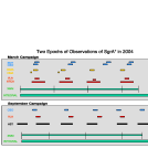
Figure 1: A schemetic diagram showing different telescopes used in both observing campaigns. The width of individual observing period is not scaled.

The campaign consisted of two epochs of observations starting March 28, 2004 and 154 days later on August 31, 2004. The observations with various telescopes lasted for about four days in each epoch. The first epoch employed the following observatories: XMM-Newton, INTEGRAL, Very Large Array (VLA) of the National Radio Astronomy Observatory, Caltech Submillimeter Observatory (CSO), Submillimeter Telescope (SMT), Nobeyama Array (NMA), Berkeley Illinois Maryland Array (BIMA) and Australian Telescope Compact Array (ATCA). The second epoch observations used only five observatories: XMM-Newton, INTEGRAL, VLA, Hubble Space Telescope (HST) Near Infrared Camera and Multi-Object Spectrometer (NICMOS) and CSO. Figure 1 shows a schematic diagram showing all of the instruments that were used during the two observing campaigns. A more detailed account of radio data will be presented elsewhere (Roberts et al. 2005)

An outburst from an eclipsing binary CXOGCJ174540.0-290031 took place prior to the first epoch and consequently confused the variability analysis of Sgr A*, especially in low-resolution data (Bower et al. 2005; Muno et al. 2005; Porquet et al. 2005). Thus, most of the analysis presented here concentrates on our second epoch observations. In addition, ground-based near-IR observations of Sgr A* using the VLT were corrupted in both campaigns due to bad weather. Thus, the only near-IR data was taken using NICMOS of HST in the second epoch. The structure of this paper is as follows. We first concentrate on the highlights of variability results of Sgr A* in different wavelength regimes in an increasing order of wavelength, followed by the correlation of the light curves, the power spectrum analysis of the light curves in near-IR wavelengths and construction of its multiwavelength spectrum. We then discuss the emission mechanism responsible for the flare activity of Sgr A*.

2 Observations

2.1 X-ray and $\gamma$-ray Wavelengths: XMM-Newton and INTEGRAL

One of us (A.G.) was the principal investigator who was granted observing time using the XMM-Newton and INTEGRAL observatories to monitor the spectral and temporal properties of Sgr A*. These high-energy observations led the way for other simultaneous observations. Clearly, X-ray and $\gamma$-ray observations had the most complete time coverage during the campaign. A total of 550 ks observing time or $\approx$1 week was given to XMM observations, two orbits (about 138 ks each) in each of two epochs (Belanger et al. 2005a; Proquet et al. 2005). Briefly, these X-ray observations discovered two relatively strong flares equivalent of 35 times the quiescent X-ray flux of Sgr A* in each of the two epochs, with peak X-ray fluxes of 6.5 and $6\times 10^{-12}$ ergs s^-1 cm^-2 between 2-10 keV. These fluxes correspond to X-ray luminosity of 7.6 and 7.7 $\times 10^{34}$ ergs s^-1 at the distance of 8 kpc, respectively. The duration of these flares were about 2500 and 5000 s. In addition, the eclipsing X-ray binary system CXOGC174540.0-290031 localized within 3^′′ of Sgr A* was also detected in both epochs (Porquet et al. 2005). Initially, the X-ray emission from this transient source was identified by Chandra observation in July 2004 (Muno et al. 2005) before it was realized that its X-ray and radio emission persisted during the the first and second epochs of the observing campaign (Bower et al. 2005; Belanger et al. 2005a; Porquet et al. 2005).

Soft $\gamma$-ray observations using INTEGRAL detected a steady source IGRJ17456-2901 within $1^{\prime}$ of Sgr A* between 20-120 keV (Belanger et al. 2005b). (Note that the PSF of IBIS/ISGRI of INTEGRAL is 13^′.) IGRJ17456-2901 is measured to have a flux 6.2$\times 10^{-11}$ erg s^-1 cm^-2 between 20–120 keV corresponding to a luminosity of 4.76$\times 10^{35}$ erg s^-1. During the time that both X-ray flares occurred, INTEGRAL missed observing Sgr A*, as this instrument was passing through the radiation belt exactly during these X-ray flare events (Belanger et al. 2005b).

2.2 Near-IR Wavelengths: HST NICMOS

2.2.1 Data Reductions

As part of the second epoch of the 2004 observing campaign, 32 orbits of NICMOS observations were granted to study the light curve of Sgr A* in three bands over four days between August 31 and September 4, 2004. Given that Sgr A* can be observed for half of each orbit, the NICMOS observations constituted an excellent near-IR time coverage in the second epoch observing campaign. NICMOS camera 1 was used, which has a field of view of $\sim 11^{\prime\prime}$ and a pixel size of 0.043${}^{\prime\prime}.$ Each orbit consisted of two cycles of observations in the broad H-band filter (F160W), the narrow-band Pa$\alpha$ filter at 1.87$\mu$m (F187N), and an adjacent continuum band at 1.90$\mu$m (F190N). The narrow-band F190N line filter was selected to search for 1.87$\mu$m line emission expected from the combination of gravitational and Doppler effects that could potentially shift any line emission outside of the bandpass of the F187N. Each exposure used the MULTIACCUM readout mode with the predefined STEP32 sample sequence, resulting in total exposure times of $\sim$7 minutes per filter with individual readout spacings of 32 seconds.

The IRAF routine “apphot” was used to perform aperture photometry of sources in the NICMOS Sgr A* field, including Sgr A* itself. For stellar sources the measurement aperture was positioned on each source using an automatic centroiding routine. This approach could not be used for measuring Sgr A*, because its signal is spatially overlapped by that of the orbiting star S2. Therefore the photometry aperture for Sgr A* was positioned by using a constant offset from the measured location of S2 in each exposure. The offset between S2 and Sgr A* was derived from the orbital parameters given by Ghez et al. (2003). The position of Sgr A* was estimated to be 0.13^′′ south and 0.03^′′ west of S2 during the second epoch observing campaign. To confirm the accuracy of the position of Sgr A*, two exposures of Sgr A* taken before and during a flare event were aligned and subtracted, which resulted in an image showing the location of the flare emission. We believe that earlier NICMOS observations may have not been able to detect the variability of Sgr A* due to the closeness of S2 to Sgr A* (Stolovy et al. 1999).

At 1.60$\mu$m, the NICMOS camera 1 point-spread function (PSF) has a full-width at half maximum (FWHM) of  0.16^′′ or  3.75 pixels. Sgr A* is therefore located at approximately the half-power point of the star S2. In order to find an optimal aperature size of Sgr A*, excluding signal from S2 which allowed enough signal from Sgr A* for a significant detection, several sizes were measured. A measurement aperture radius of 2 pixels (diameter of 4 pixels) was found to be a suitable compromise.

We have made photometric measurements in the F160W (H-band) images at the 32 second intervals of the individual exposure readouts. For the F187N and F190N images, where the raw signal-to-noise ratio is lower due to the narrow filter bandwidth, the photometry was performed on readouts binned to $\sim$3.5 minute intervals. The standard deviation in the resulting photometry is on the order of $\sim$0.002 mJy at F160W (H-band) measurements and $\sim$0.005 mJy at F187N and F190N.

The resulting photometric measurements for Sgr A* show obvious signs of variability (as discussed below), which we have confirmed through comparison with photometry of numerous nearby stars. Comparing the light curves of these objects, it is clear that sources such as S1, S2, and S0-3 are steady emitters, confirming that the observed variability of Sgr A* is not due to instrumental systematics or other effects of the data reduction and analysis. For example, the light curves of Sgr A* and star S0-3 in the F160W band are shown in Figure 2a. It is clear that the variability of Sgr A* seen in three of the six time intervals is not seen for S0-3. The light curve of IRS 16SW, which is known to be a variable star, has also been constructed and is clearly consistent with ground-based observations (Depoy et al. 2004).

2.2.2 Photometric Light Curves and Flare Statistics

The thirty-two HST orbits of Sgr A* observations were distributed in six different observing time windows over the course of four days of observations. The detected flares are generally clustered within three different time windows, as seen in Figure 2b. This figure shows the photometric light curves of Sgr A* in the 1.60, 1.87, and 1.90$\mu$m NICMOS bands, using a four pixel diameter measurement aperture. The observed “quiescent” emission level of Sgr A* in the 1.60$\mu$m band is $\sim$0.15 mJy (uncorrected for reddening). During flare events, the emission is seen to increase by 10% to 20% above this level. In spite of the somewhat lower signal-to-noise ratio for the narrow-band 1.87 and 1.90$\mu$m data, the flare activity is still detected in all bands.

Figure 3a presents detailed light curves of Sgr A* in all three NICMOS bands for the three observing time windows that contained active flare events, which corresponds to the second, fourth, and sixth observing windows. An empirical correction has been applied to the fluxes in 1.87 and 1.90 $\mu$m bands in order to overlay them with the 1.60$\mu$m band data. The appropriate correction factors were derived by computing the mean fluxes in the three bands during the observing windows in which no flares were seen. This lead us to scale down the observed fluxes in the 1.87 and 1.90$\mu$m bands by factors of 3.27 and 2.92, respectively, in order to compare the observed 1.60$\mu$m band fluxes. All the data are shown as a time-ordered sequence in Figure 3a.

Flux variations are detected in all three bands in the three observing windows shown in Figure 3a. The bright flares (top and middle panels) show similar spectral and temporal behaviors, both being separated by about two days. These bright flares have multiple components with flux increases of about 20% and durations ranging from 2 to 2.5 hours and dereddened peak fluxes of $\sim$10.9 mJy at 1.60$\mu$m. The weak flares during the end of the fourth observing window (middle panel) consist of a collection of sub-flares lasting for about 2–2.5 hours with a flux increase of only 10%. The light curve from the last day of observations, as shown in the bottom panel of Figure 3a, displays the highest level of flare activity over the course of the four days. The dereddened peak flux at 1.6$\mu$m is $\sim$11.1 mJy and decays in less than 40 minutes. Another flare starts about 2 hours later with a rise and fall time of about 25 minutes, with a peak dereddened flux of 10.5 mJy at 1.6$\mu$m. There are a couple of instances where the flux changed from ”quiescent” level to peak flare level or vice versa in the span of a single (1 band) exposure, which is on the order of $\sim$7 minutes. For our 1.6 micron fluxes, Sgr A* is 0.15 mJy (dereddened) above the mean level approximately 34% of the time. For a somewhat more stringent higher significant level of 0.3 mJy above the mean, the percentage drops to about 23%.

Dereddened fluxes quoted above were computed using the appropriate extinction law for the Galactic center (Moneti et al. 2001) and the Genzel et al. (2003) extinction value of A(H)=4.3 mag. These translate to extinction values for the NICMOS filter bands of A(F160W)=4.5 mag, A(F187N)=3.5 mag, and A(F190N)=3.4 mag, which then correspond to corrections factors of 61.9, 24.7, and 23.1. Applying these corrections leaves the 1.87 and 1.90$\mu$m fluxes for Sgr A* at levels of $\sim$27% and $\sim$7%, respectively, above the fluxes in the 1.60 $\mu$m band. This may suggest that the color of Sgr A* is red. However, applying the same corrections to nearby stars, such as S2 and S0-3, the results are essentially the same as that of Sgr-A*, namely, the 1.87$\mu$m fluxes are still high relative to the fluxes at 1.60 and 1.90$\mu$m. This discrepancy in the reddening correction is likely to be due to a combination of factors. One is the shape of the combined spectrum of Sgr A* and the shoulder of S2, as the wings of S2 cover the position of Sgr A* . The other is the diffuse background emission from stars and ionized gas in the general vicinity of Sgr A*, as well as the derivation of the extinction law based on ground-based filters, which could be different than the NICMOS filter bands. Due to these complicating factors, we chose to use the empirically-derived normalization method described above when comparing fluxes across the three NICMOS bands.

We have used two different methods to determine the flux of Sgr A* when it is flaring. One is to measure directly the peak emission at 1.6$\mu$m during the flare to $\approx$0.18 mJy. Using a reddening correction of about a factor of 62, this would translate to $\sim$10.9 mJy. Since we have used an aperture radius of only 2 pixels, we are missing a very significant fraction of the total signal coming from Sgr A*. In addition, the contamination by S2 will clearly add to the measured flux of Sgr A*. Not only are we not measuring all the flux from Sgr A* using our 2-pixel radius aperture, but more importantly, we’re getting a large (but unknown) amount of contamination from other sources like S2. The second method is to determine the relative increase in measured flux which can be safely attributed to Sgr A* (since we assume that the other contaminating sources like S2 don’t vary). The increase in 1.6$\mu$m emission that we have observed from Sgr A* during flare events is $\sim$0.03 mJy, which corresponds to a dereddened flux of $\sim$1.8 mJy. Based on photometry of stars in the field, we have derived an aperture correction factor of $\sim$2.3, which will correct the fluxes measured in our 2-pixel radius aperture up to the total flux for a point source. Thus, the increase in Sgr A* flux during a flare increases to a dereddened value of $\sim$4.3 mJy. Assuming that all of the increase comes from just Sgr-A*, and then adding that increase to the 2.8 mJy quiescent flux (Genzel et al. 2003), then we measure a peak dereddened H-band flux of $\sim$7.5 mJy during a flare. However, recent detection of 1.3 mJy dereddened flux at 3.8$\mu$m from Sgr A* (Ghez et al. 2005) is lower than the lowest flux at H band that had been reported earlier (Ghez et al. 2005). This implies that the flux of Sgr A* may be fluctuating constantly and there is no quiescent state in near-IR band. Given the level of uncertainties involved in both techniques, we have used the first method of measuring the peak flux which is adopted as the true flux of Sgr A* for the rest of the paper. If the second method is used, the peak flux of Sgr A* should be lowered by a factor of $\sim$0.7.

We note that the total amount of time that flare activity has been detected is roughly 30–40% of the total observation time. It is remarkable that Sgr A* is active at these levels for such a high fraction of the time at near-IR wavelengths, especially when compared to its X-ray activity, which has been detected on the average of once a day or about 1.4 to 5% of the observing time depending on different instruments (Baganoff et al. 2003; Belanger et al. 2005a). In fact, over the course of one week of observations in 2004, XMM detected only two clusters of X-ray flares. Recent detection of 1.3 mJy dereddened flux at 3.8$\mu$m from Sgr A* is lower than the lowest flux at H band that had been reported earlier (Ghez et al. 2005). This measurement when combined with our variability analysis is consistent with the conclusion that the near-IR flux of Sgr A* due to flare activity is fluctuating constantly at a low level and that there is no quiescent flux.

Figure 3b shows a histogram plot of the detected flares and the noise as well as the simultaneous 2-Gaussian fit to both the noise and the flares. In the plot the dotted lines are the individual Gaussians, while the thick dashed line is the sum of the two. The variations near zero is best fitted with a Gaussian, which is expected from random noise in the observations, while the positive half of the histogram shows a tail extending out to $\sim$2 mJy above the mean, which represents the various flare detections. The flux values are dereddened values within the 4-pixel diameter photometric aperture at 1.60$\mu$m.

The ”flux variation” values were computed by first computing the mean F160W flux within one of our ”quiescent” time windows and then subtracting this quiescent value from all the F160W values in all time periods. So these values represent the increase in flux relative to the mean quiescent. The parameters of the fitted Gaussian for the flares is 10.9, 0.47$\pm$0.3 mJy, 1.04$\pm$0.5 mJy corresponding to the amplitude, center and FWHM, respectively. The total area of the individual Gaussians are 26.1 and 12.0 which gives the percentage of the area of the flare Gaussian, relative to the total of the two, to be $\sim$31%. This is consistent with our previous estimate that flares occupy 30-40% of the observing time.

A mean quiescent 1.6$\mu$m flux of 0.15 mJy (observed) corresponds to a dereddened flux of $\sim$9.3 mJy within a 4-pixel diameter aperture. The total flux for a typical flare event (which gives an increase of 0.47 mJy) would be $\sim$9.8 mJy. But of course all of these measurements refer to the amount of flux collected in a 4-pixel diameter aperture, which includes some contribution from S2 star and at the same time does not include all the flux of Sgr A*. If we include the increase associated with a typical flare, which excludes any contribution from S2, and apply the aperture correction factor of 2.4 which accounts for the amount of missing light from Sgr A*, then the typical flux of of 0.47 mJy corresponds to a value of 1.13 mJy. If we then use the quiescent flux of Sgr A* at H-band (Genzel et al. 2003), the absolute flux a typical flare at 1.6$\mu$m is estimated to be $\sim$3.9 mJy. The energy output per event from a typical flare with a duration of 30 minutes is then estimated to be $\sim$10³⁸ ergs. The Gaussian nature of the flare histogram suggests that this estimate corresponds to the characteristic energy scale of the accelerating events (If we use a typical flux of a flare $\sim$9.8 mJy, then the energy scale increases by a factor of 2.5).

In terms of power-law versus Gaussian fit, the power-law fit to the flare portion only gave a $\chi^{2}$=2.6 and rms=1.6, while the Gaussian fit to the flare part only gives a $\chi^{2}$=1.6 and rms=1.2 (better in both). With the limited data we have, we believe that it is difficult to fit a power-law to the flare portion along with a Gaussian to the noise peak at zero flux, because the power-law fit continues to rise dramatically as it approaches to zero flux, which then swamps the noise portion centered at zero.

During the relatively quiescent periods of our observations, the observed 1.6 $\mu$m fluxes have a 1$\sigma$ level of $\sim$0.002-0.003 mJy. Looking at the periods during which we detected obvious flares, an increase of $\sim$0.005 mJy is noted. This is about 2$\sigma$ relative to the observation-to-observation scatter quoted above ($\sim$0.002 mJy). To compare these values to the ground-based data using the same reddening correction as Genzel et al. (2003), our 1-$\sigma$ scatter would be about $\sim$0.15 mJy at 1.6 $\mu$m, with our weakest detected flares having a flux $\sim$0.3 mJy at 1.6 $\mu$m. Genzel et al. report H-band weakest detectable variability at about the 0.6 mJy level. Thus, the HST 1-$\sigma$ level is about a factor of 4 better and the weakest detectable flares about a factor of 2 better than ground-based observations.

2.2.3 Power Spectrum Analysis

Motivated by the report of a 17-minute periodic signal from Sgr A* in near-IR wavelengths (Genzel et al. 2003), the power spectra of our unevenly-spaced near-IR flares were measured using the Lomb-Scargle periodogram (e.g., Scargle 1982). There are certain possible artificial signals that should be considered in periodicity analysis of HST data. One is the 22-minute cycle of the three filters of NICMOS observations. In addition, the orbital period of HST is 92 minutes, 46 minutes of which no observation can be made due to the Earth’s occultation. Thus, any signals at the frequencies corresponding to the inverse of these periods, or their harmonics, are of doubtful significance. In spite of these limitations the data is sampled and characterized well for the periodic analysis. In order to determine the significance of power at a given frequency, we employed a Monte Carlo technique to simulate the power-law noise following an algorithm that has been applied to different data sets (Timmer & König 1995; Mauerhan et al. 2005). 5000 artificial light curves were constructed for each time segment. Each simulated light curve contained red noise, following P($f)\propto f^{-\beta}$, and was forced to have the same variance and sampling as the original data.

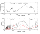
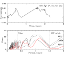
Figure 4: (a, top) The top and bottom boxes of the top panel show the light curves and the corresponding power spectra of the residual flux of Sgr A* during the 2nd observing time window when flare activity was detected. The dashed lines show the significance of the power spectrum at 50, 95 and 99% confidence levels. (b, bottom) Similar to (a) except that the light curve and the power spectrum of the fourth observing time window are shown.

Figures 4a,b show the light curves, power spectra, and envelopes of simulated power spectra for the flares during the 2nd and 4th observing time windows. The flare activity with very weak signal-to-noise ratio at the end of the 4th observing window was not included in the power spectrum analysis. The flares shown in Figures 4a,b are separated by about two days from each other and the temporal and spatial behavior of of their light curves are similar. Dashed curves on each figure indicate the envelope below which 99% (higher curve), 95% (middle curve), and 50% (lower curve) of the simulated power spectra lie. These curves show ripples which incorporate information about the sampling properties of the lightcurves.

The vertical lines represent the period of an HST orbit and the period at which the three observing filters were cycled. The only signals which appear to be slightly above the 99% light curve of the simulated power spectrum are at 0.55$\pm$0.03 hours, or 33$\pm$2 minutes. The power spectrum of the sixth observing window shows similar significance near 33 minutes, but also shows similar significance at other periods near the minima in the simulated lightcurves. We interpret this to suggest that the power in the sixth observation is not well-modeled as red noise.

We compared the power spectrum of the averaged data from three observing windows using a range of $\beta$ from 1 to 3. The choice of $\beta$=2 shows the best overall match between the line enclosing 50% of the simulated power spectra and the actual power spectrum. A $\beta$ of 3 is not too different in the overall fit to that of $\beta=2$. For the choice of $\beta$=1, significant power at longer time scales becomes apparent. However, the significance of longer periods in the power spectrum disappears when $\beta=2$ was selected, thus we take $\beta$=2 to be the optimal value for our analysis.

The only signal that reaches a 99% significance level is the 33-minute time scale. This time scale is about twice the 17-minute time scale that earlier ground-based observations reported (Genzel et al. 2003). There is no evidence for any periodicity at 17 minutes in our data. The time scale of about 33 minutes roughly agrees with the timescales on which the flares rise and decay. Similarly, the power spectrum analysis of X-ray data show several periodicities, one of which falls within the 33-minute time scale of HST data (Aschenbach et al. 2004; Aschenbach 2005). However, we are doubtful whether this signal indicates a real periodicity. This signal is only slightly above the noise spectrum in all of our simulations and is at best a marginal result. It is clear that any possible periodicities need to be confirmed with future HST observations with better time coverage and more regular time spacing. Given that the low-level amplitude variability that is detected here with HST data is significantly better than what can be detected with ground-based telescopes, additional HST observations are still required to fully understand the power spectrum behavior of near-IR flares from Sgr A*.

2.3 Submillimeter Wavelengths: CSO and SMT

2.3.1 CSO Observations at 350, 450, 850 $\mu$m

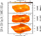
Figure 5: (a) The light curves of Sgr A* at 850 $\mu$m with 1-$\sigma$ error bars during the second observing campaign with CSO. The integration time for each individual data point is 20min (top panel). (b) The maps of Sgr A* and the orbiting circumnuclear rings at 850$\mu$m in two different times during the flare. The subtracted map to the right shows Sgr A* is the only significant source that was variable.

Using CSO with SHARC II, Sgr A* was monitored at 450 and 850 $\mu$m in both observing epochs (Dowell et al. 2004). Within the 2 arcminute field of view of the CSO images, a central point source coincident with Sgr A* is visible at 450 and 850 $\mu$m wavelengths having spatial resolutions of 11^′′ and 21^′′, respectively. Figure 5a shows the light curves of Sgr A* in the second observing epoch with 1$\sigma$ error bars corresponding to 20min of integration. The 1$\sigma$ error bars are noise and relative calibration uncertainty added in quadrature. Absolute calibration accuracy is about 30% (95% confidence). During the first epoch, when a transient source appeared a few arcseconds away from Sgr A*, no significant variability was detected. The flux density of Sgr A* at 850 $\mu$m is consistent with the SMT flux measurement of Sgr A* on March 28, 2004, as discussed below. During this epoch, Sgr A* was also observed briefly at 350 $\mu$m on April 1 and showed a flux density of 2.7$\pm$0.8 Jy.

The light curve of Sgr A* in the second epoch, presented in Figure 5a, shows only $\sim$25% variability at 450 $\mu$m. However, the flux density appears to vary at 850$\mu$m in the range between 2.7 and 4.6 Jy over the course of this observing campaign. Since the CSO slews slowly, and we need all of the Sgr A* signal-to-noise, we only observe calibrators hourly. The hourly flux of the calibrators as a function of atmospheric opacity shows $\sim$30% peak-to-peak uncertainty for a particular calibration source and a 10% relative calibration uncertainty (1$\sigma$) for the CSO 850 micron data.

We note the presence of remarkable flare activity at 850 $\mu$m on the last day of the observation during which a peak flux density of 4.6 Jy was detected with a S/N = 5.4. The reality of this flare activity is best demonstrated in a map, shown in Figure 5b, which shows the 850$\mu$m flux from well-known diffuse features associated with the southern arm of the circumnuclear ring remaining constant, while the emission from Sgr A* rises to 4.6 Jy during the active period. The feature of next highest significance after Sgr A* in the subtracted map showing the variable sources is consistent with noise with S/N = 2.5.

2.3.2 SMT Observations at 870 $\mu$m

Sgr A^∗ was monitored in the 870$\mu$m atmospheric window using the MPIfR 19 channel bolometer on the Arizona Radio Observatory (ARO) 10m HHT telescope (Baars et al. 1999). The array covers a total area of 200^′′ on the sky, with the 19 channels (of 23^′′ HPBW) arranged in two concentric hexagons around the central channel, with an average separation of 50^′′ between any adjacent channels. The bolometer is optimized for operations in the 310-380 GHz (970-790 $\mu$m) region, with a maximum sensitivity peaking at 340 GHz near 870 $\mu$m.

The observations were carried out in the first epoch during the period March 28-30th, 2004 between 11-16h UT. Variations of the atmospheric optical depth at 870$\mu$m were measured by straddling all observations with skydips. The absolute gain of the bolometer channels was measured by observing the planet Uranus at the end of each run. A secondary flux calibrator, i.e. NRAO 530, was observed to check the stability and repeatability of the measurements. All observations were carried out with a chopping sub-reflector at 4Hz and with total beam-throws in the range 120${}^{\prime\prime}-180^{\prime\prime}$, depending on a number of factors such as weather conditions and elevation.

As already noted above, dust around Sgr A^∗ is clearly contaminating our measurements at a resolution of 23^′′. Due to the complexity of this field, the only possibility to try to recover the uncontaminated flux is to fit several components to the brightness distribution, assuming that in the central position, there is an unresolved source, surrounded by an extended smoother distribution. We measured the average brightness in concentric rings (of 8^′′ width) centered on Sgr A^∗ in the radial distance range 0-80^′′. The averaged radial profile was then fitted with several composite functions, but always included a point source with a PSF of the order of the beam-size. The best fit for both the central component and a broader and smoother outer structure gives a central (i.e., Sgr A^∗) flux of 4.0$\pm$0.2Jy in the first day of observation on March 28, 2004. The CSO source flux fitting, as described earlier, and HHT fitting are essentially the same.

Due to bad weather, the scatter in the measured flux of the calibrator NRAO 530 and Sgr A* was high in the second and third days of the run. Thus, the measurements reported here are achieved only for the first day with the photometric precision $\leq$12$\%$ for the calibrator. The flux of NRAO 530 at 870$\mu$m during this observation was 1.2$\pm$0.1 Jy.

2.4 Radio Wavelengths: NMA, BIMA, VLA & ATCA

2.4.1 NMA Observations at 2 &3mm

NMA was used in the first observing epoch to observe Sgr A* at 3 mm (90 GHz) and 2 mm (134 GHz), as part of a long-term monitoring campaign (Tsutsumi, Miyazaki & Tsuboi 2005). The 2 and 3 mm flux density were measured to be 1.8$\pm$0.4 and 2.0$\pm$0.3 Jy on March 31 and April 1, 2004, respectively, during 2:30-22:15 UT. These authors had also reported a flux density of 2.6$\pm$0.5 Jy at 2 mm on March 6, 2004. This observation took place when a radio and X-ray transient near Sgr A* was active. Thus, it is quite possible that the 2 mm emission toward Sgr A* is not part of a flare activity from Sgr A* but rather due to decaying emission from a radio/X-ray transient which was first detected by XMM and VLA on March 28, 2004.

2.4.2 BIMA Observations at 3mm

Using nine telescopes, BIMA observed Sgr A* at 3 mm (85 GHz, average of two sidebands at 82.9 and 86.3 GHz) for five days between March 28 and April 1, 2004 during 11:10-15:30 UT . Detailed time variability analysis is given elsewhere (Roberts et al. 2005). The flux densities on March 28 and April 1 show average values of 1.82$\pm$0.16 and 1.87$\pm$0.14 at $\sim$3 mm, respectively. These values are consistent with the NMA flux values within errors. No significant hourly variability was detected.

The presence of the transient X-ray/radio source a few arcseconds south of Sgr A* during this epoch complicates time variability analysis of BIMA data since the relatively large synthesized beam (8$.\!\!^{\prime\prime}$2 $\times$ 2$.\!\!^{\prime\prime}$6) changes during the course of the observation. Thus, as the beam rotates throughout an observation, flux included from Sgr A West and the radio transient may contaminate the measured flux of Sgr A*.

2.4.3 VLA Observations at 7mm

Using the VLA, Sgr A* was observed at 7mm (43 GHz) in the first and second observing epochs. In each epoch, observations were carried out on four consecutive days, with an average temporal coverage of about 4 hr per day. In order to calibrate out rapid atmospheric changes, these observations used a new fast switching technique for the first time to observe time variability of Sgr A*. Briefly, these observations used the same calibrators (3C286, NRAO 530 and 1820-254). The fast switching mode rapidly alternated between Sgr A* (90sec) and the calibrator 1820-254 (30sec). Tipping scans were included every 30 min to measure and correct for the atmosphere opacity. In addition, pointing was done by observing NRAO 530. After applying high frequency calibration, the flux of Sgr A* was determined by fitting a point source in the uv plane ($>$100 k$\lambda$). As a check, the variability data were also analyzed in the image plane, which gave similar results.

The results of the analysis at 7mm clearly indicate a 5-10% variability on hourly time scales, in almost all the observing runs. A power spectrum analysis, similar to the statistical analysis of near-IR data presented above, was also done at 7mm. Figure 6a shows typical light curves of NRAO 530 and Sgr A* in the top two panels at 7mm. Similar behavior is found in a number of observations during 7mm observations in both epochs. It is clear that the light curve starts with a peak (or that the peak preceded the beginning of the observation) followed by a decay with a duration of 30 minutes to a quiescent level lasting for about 2.5 hours.

2.4.4 ATCA Observations at 1.7 and 1.5cm

At the ATCA, we used a similar observing technique to that of our VLA observations, involving fast switching between the calibrator and Sgr A* simultaneously at 1.7 (17.6 GHz) and 1.5 cm (19.5 GHz). Unlike ground based northern hemisphere observatories that can observe Sgr A* for only 5 hours a day (such as the VLA), ATCA observed Sgr A* for 4 $\times$ 12 hours in the first epoch. In spite of the possible contamination of variable flux due to interstellar scintillation toward Sgr A* at longer wavelengths, similar variations in both 7 mm and 1.5 cm are detected. Figure 6b shows the light curve of Sgr A* and the corresponding calibrator during a 12-hour observation with ATCA at 1.7cm. The increase in the flux of Sgr A* is seen with a rise and fall time scale of about 2 hours. The 1.5, 1.7 cm and 7 mm variability analysis is not inconsistent with the time scale at which significant power has been reported at 3 mm (Mauerhan et al. 2005). Furthermore, the time scales for rise and fall of flares in radio wavelengths are longer than in the near-IR wavelengths discussed above.

3 Correlation Study

3.1 Epoch 1

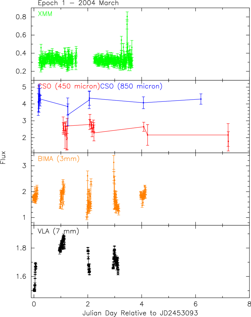
Figure 7: The simultaneous X-ray, submillimeter, millimeter and radio emission from Sgr A* based on the first epoch of observations using XMM, CSO, BIMA and VLA.

Figure 7 shows the simultaneous light curves of Sgr A* during the first epoch in March 2004 based on observations made with XMM, CSO at 450 and 850 $\mu$m, BIMA at 3 mm and VLA at 7 mm. The flux of Sgr A* remained constant in submillimeter and millimeter wavelengths throughout the first epoch, while we observed an X-ray flare (top panel) at the end of the XMM observations and hourly variations in radio wavelengths (bottom panel) at a level 10-20%. This implies that the contamination from the radio and X-ray transient CXOGCJ174540.0-290031, which is located a few arcseconds from Sgr A*, is minimal, thus the measured fluxes should represent the quiescent flux of Sgr A*. These data are used to make a spectrum of Sgr A*, as discussed in section 5. As for the X-ray flare, there were no simultaneous observations with other instruments during the period in which the X-ray flare took place. Thus, we can not state if there were any variability at other wavelengths during the X-ray flare in this epoch.

3.2 Epoch 2

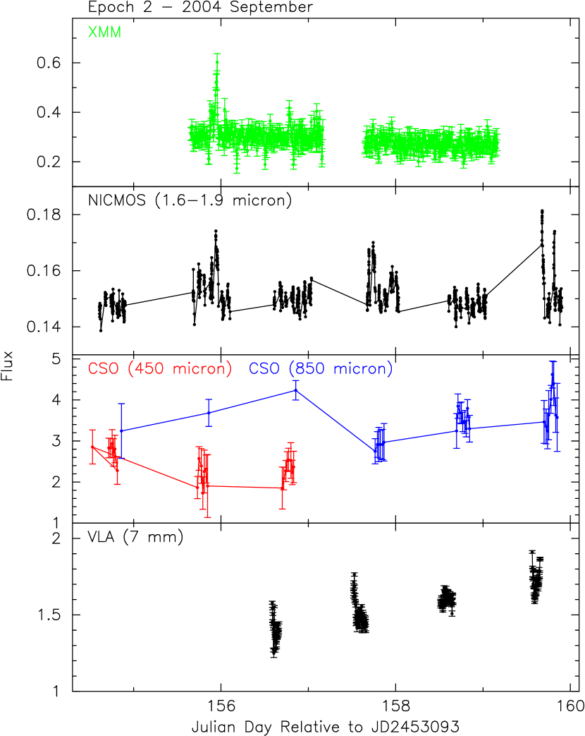
Figure 8: The simultaneous X-ray, near-IR, submillimeter, and radio emission from Sgr A* based on the second epoch of observations using XMM, HST, CSO, and VLA. The 8h periodic dips detected in the X-ray light curve are due to the eclipses of the transient, as described in Porquet et al. 2005).

Figure 8 shows the simultaneous light curve of Sgr A* based on the second epoch of observations using XMM, HST, CSO and VLA. Porquet et al. (2005) noted clear 8-hour periodic dips due to the eclipses of the transient as seen clearly in the XMM light curve. Sgr A* shows clear variability at near-IR and submillimeter wavelengths, as discussed below.

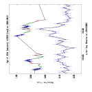
Figure 9: The simultaneous near-IR (top plot) and X-ray (bottom plot) light curves during which flares were detected in the second epoch of the observing campaign. The near-IR flares are detected in the 2nd observing window, as shown in Figure 3a. The vertical axis shows the observed flux density in near-IR wavelengths whereas the observed count rate in X-ray wavelengths. The F187N (green color) and F190N (red color) filter data are sampled at 128 sec intervals whereas the F160W (blue color) are sampled every 32 sec. The X-ray data have 200-second time resolution.

One of the most exciting results of this observing campaign is the detection of a cluster of near-IR flares in the second observing window which appears to have an X-ray counterpart. The long temporal coverage of XMM-Newton and HST observations have led to the detection of a simultaneous flare in both bands. However, the rest of the near-IR flares detected in the fourth and sixth observing windows (see Figure 3) show no X-ray counterparts at the level that could be detected with XMM. The two brightest near-IR flares in the second and fourth observing windows are separated by roughly two days and appear to show similar temporal and spatial behaviors. Figure 9 shows the simultaneous near-IR and X-ray emission with an amplitude increase of $\sim$15% and 100% for the peak emission, respectively. We believe that these flares are associated with each other for the following reasons. First, X-ray and near-IR flares are known to occur from Sgr A* as previous high resolution X-ray and near-IR observations have pinpointed the origin of the flare emission. Although near-IR flares could be active up to 40% of time, the X-ray flares are generally rare with a 1% probablity of occurance based on a week of observation with XMM. Second, although the chance coincidence for a near-IR flare to have an X-ray counterpart could be high but what is clear from Figure 9 is the way that near-IR and X-ray flares track each other on a short time. Both the near-IR and X-ray flares show similar morphology in their light curves as well as similar duration with no apparent delay. This leads us to believe that both flares come from the same region close to the event horizon of Sgr A*. The X-ray light curve shows a double peaked maximum flare near Day 155.95 which appears to be remarkably in phase with the near-IR strongest double peaked flares, though with different amplitudes. We can also note similar trend in the sub-flares noted near Day 155.9 in Figure 9 where they show similar phase but different amplitudes. Lastly, since X-ray flares occur on the average once a day, the lack of X-ray counterparts to other near-IR flares indicates clearly that not all near-IR flares have X-ray counterparts. This fact has important implications on the emission mechanism, as described below.

With the exception of the September 4, 2004 observation toward the end of the second observing campaign, the large error bars of the submillimeter data do not allow us to determine short time scale variability in this wavelength domain with high confidence. We notice a significant increase in the 850$\mu$m emission about 22 hours after the simultaneous X-ray/near-IR flare took place, as seen in Figure 8. We also note the highest 850$\mu$m flux in this campaign 4.62$\pm$0.33 Jy which is detected toward the end of the submillimeter observations. This corresponds to a 5.4$\sigma$ increase of 850$\mu$m flux.

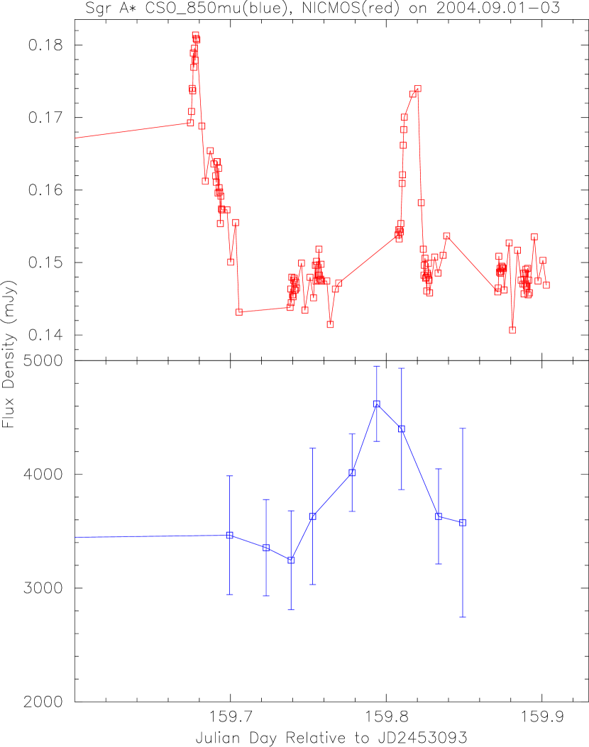
Figure 10: The simultaneous near-IR and 850$\mu$m light curves showing flares detected in the second epoch of the observing campaign. The near-IR flares correspond to the 6th observing window, as shown in Figure 3. There are no X-ray observations during the period when these flares took place.

Figure 10 shows simultaneous light curves of Sgr A* at 850$\mu$m and near-IR wavelengths. The strongest near-IR flare occurred at the beginning of the 6th observing window with a decay time of about 40 minutes followed by the second flare about 200 minutes later with a decay time of about 20 minutes. The submillimeter light curve shows a peak about 160 minutes after the strongest near-IR flare that was detected in the second campaign. The duration of the submillimeter flare is about two hours. Given that there is no near-IR data during one half of every HST orbit and that the 850$\mu$m data were sampled every 20 minutes compared to 32sec sampling rate in near-IR wavelengths, it is not clear whether the submillimeter data is correlated simultaneously with the second bright near-IR flare, or is produced by the first near-IR flare with a delay of 160 minutes, as seen in Figure 10. What is significant is that submillimeter data suggests that the 850$\mu$m emission is variable and is correlated with the near-IR data. Using optical depth and polarization arguments, we argue below that the submillimeter and near-IR flares are simultaneous.

4 Emission Mechanism

4.1 X-ray and Near-IR Emission

Theoretical studies of accretion flow near Sgr A* show that the flare emission in near-IR and X-rays can be accounted for in terms of the acceleration of particles to high energies, producing synchrotron emission as well as ICS (e.g., Markoff et al. 2001; Liu & Melia 2001; Yuan, Markoff & Falcke 2002; Yuan, Quataert & Narayan 2003, 2004). Observationally, the near-IR flares are known to be due to synchrotron emission based on spectral index and polarization measurements (e.g., Genzel et al. 2003 and references therein). We argue that the X-ray counterparts to the near-IR flares are unlikely to be produced by synchrotron radiation in the typical $\sim 10$ G magnetic field inferred for the disk in Sgr A* for two reasons. First, emission at 10 keV would be produced by 100 GeV electrons, which have a synchrotron loss time of only 20 seconds, whereas individual X-ray flares rise and decay on much longer time scales. Second, the observed spectral index of the X-ray counterpart, $\alpha=0.6$ ($S_{\nu}\propto\nu^{-\alpha=-0.6}$), does not match the near-IR to X-ray spectral index. The observed X-ray 2-10 keV flux 6$\times 10^{-12}$ erg cm^-2 s^-1 corresponds to a differential flux of 2$\times 10^{-12}$ erg cm² s^-1 keV^-1 (0.83 $\mu$Jy) at 1 keV. The extinction-corrected (for $A_{H}=4.5$ mag) peak flux density of the near-IR (1.6$\mu$m) flare is $\sim$10.9 mJy. The spectral index between X-ray and near-IR is 1.3, far steeper than the index of 0.6 determined for the X-ray spectrum.

Instead, we favor an inverse Compton model for the X-ray emission, which naturally produces a strong correlation with the near-IR flares. In this picture, submillimeter photons are upscattered to X-ray energies by the electrons responsible for the near-IR synchrotron radiation. The fractional variability at submillimeter wavelengths is less than 20%, so we first consider quiescent submillimeter photons scattering off the variable population of GeV electrons that emit in the near-IR wavelengths. In the ICS picture, the spectral index of the near-IR flare must match that of the X-ray counterpart, i.e. $\alpha$ = 0.6. Unfortunately, we were not able to determine the spectral index of near-IR flares. Recent measurements of the spectral index of near-IR flares appear to vary considerably ranging between 0.5 to 4 (Eisenhauer et al. 2005; Ghez et al. 2005). The de-reddened peak flux of 10.9 mJy (or 7.5 mJy from the relative flux measurement described in section 2.2.2) with a spectral index of 0.6 is consistent with a picture that blighter near-IR flares have harder spectral index (Eisenhauer et al. 2005; Ghez et al. 2005).

Assuming an electron spectrum extending from 3 GeV down to 10 MeV and neglecting the energy density of protons, the equipartition magnetic field is 11 G, with equipartition electron and magnetic field energy densities of $\sim$5 erg cm^-3. The electrons emitting synchrotron at 1.6$\mu$m then have typical energies of 1.0 GeV and a loss time of 35 min. 1 GeV electrons will Compton scatter 850 $\mu$m photons up to 7.8 keV, so as the peak of the emission spectrum of Sgr A* falls in the submillimeter regime, as it is natural to consider the upscattering of the quiescent submillimeter radiation field close to Sgr A*. We assume that this submillimeter emission arises from a source diameter of 10 Schwarzschild radii (R_sch), or 0.7 AU (adopting a black hole mass of 3.7$\times 10^{6}$ $M_{\odot}$). In order to get the X-ray flux, we need the spectrum of the seed photons which is not known. We make an assumption that the measured submillimeter flux (4 Jy at 850 $\mu$m), and the product of the spectrum of the near-IR emitting particles and submillimeter flux $\nu^{0.6}F_{\nu}$, are of the same order over a decade in frequency. The predicted ICS X-ray flux for this simple model is $1.2\times 10^{-12}$ erg cm^-2 s^-1 keV^-1, roughly half of the observed flux.

The second case we consider to explain the origin of X-ray emission is that near-IR photons scatter off the population of $\sim$50 MeV electrons that emit in submillimeter wavelengths. If synchrotron emission from a population of lower-energy ($\sim 50$ MeV) electrons in a similar source region (diameter $\sim 10$ R_sch, $B\sim 10$ G) is responsible for the quiescent emission at submillimeter wavelengths, then upscattering of the flare’s near-IR emission by this population will produce a similar contribution to the flux of the X-ray counterpart, and the predicted net X-ray flux $\sim 2.4\times 10^{-12}$ erg cm² s^-1 keV^-1 is similar to that observed.

The two physical pictures of ICS described above produce similar X-ray flux within the inner diameter $\sim 10$ R_sch, $B\sim 10$ G, and therefore cannot be distinguished from each other. On the other hand, if the near-IR flares arise from a region smaller than that of the quiescent submillimeter seed photons, then the first case, in which the quiescent submillimeter photons scatter off GeV electrons that emit in the near-IR, is a more likely mechanism to produce X-ray flares.

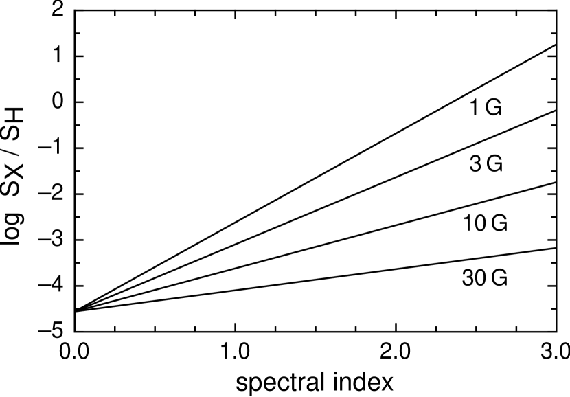
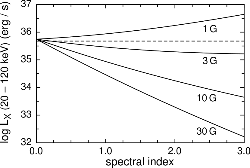
Figure 11: (a)[left] For a given magnetic field, a run of the log of the ratio of the fluxes at 1 keV and 1.6$\mu$m from Sgr A* is drawn as a function of the near-IR spectral index, for the scattering of submillimeter emission via inverse Compton. (b)[right] Similar to Figure (a) except that the vertical axis shows the log of the luminosity between 2 - 120 keV. The dashed line shows the measured flux from the inner 13^′ of the Galactic center.

The lack of an X-ray counterpart to every detected near-IR flare can be explained naturally in the ICS picture presented here. It can be understood in terms of variability in the magnetic field strength or spectral index of the relativistic particles, two important parameters that determine the relationship between the near-IR and ICS X-ray flux. A large variation of the spectral index in near-IR wavelengths has been observed (Ghez et al. 2005; Eisenhauer et al. 2005). Figure 11a shows the ratio of the fluxes at 1 keV and 1.6 $\mu$m against the spectral index for different values of the magnetic field. Note that there is a minimum field set by requiring the field energy density to be similar to or larger than the relativistic particle energy. If, as is likely, the magnetic field is ultimately responsible for the acceleration of the relativistic particles, then the field pressure must be stronger or equal to the particle energy density so that the particles are confined by the field during the acceleration process. It is clear that hardening (flattening) of the spectral index and/or increasing the magnetic field reduces the X-ray flux at 1 keV relative to the near-IR flux. On the other hand softening (steepening) the spectrum can produce strong X-ray flares. This occurs because a higher fraction of relativistic particles have lower energies and are, therefore, available to upscatter the submillimeter photons. This is consistent with the fact that the strongest X-ray flare that has been detected from Sgr A* shows the softest (steepest) spectral index (Porquet et al. 2003). Moreover, the sub-flares presented in near-IR and in X-rays, as shown in Figure 9, appear to indicate that the ratio of X-ray to near-IR flux (S_X to S_H) varies in two sets of double-peaked flares, as described earlier. We note an X-ray spike at 155.905 days has a 1.90 $\mu$m (red color) counterpart. The preceding 1.87 $\mu$m (green color) data points are all steadily decreasing from the previous flare, but then the 1.90$\mu$m suddenly increases up to at least at a level of $\sim 3\sigma$.

The flux ratio corresponding to the peak X-ray flare (Figure 9) is high as it argues that the flare has either a soft spectral index and/or a low magnetic field. Since the strongest X-ray flare that has been detected thus far has the steepest spectrum (Porquet et al. 2003), we believe that the observed variation of the flux ratio in Sgr A* is due to the variation of the spectral index of individual near-IR flares. Since most of the observed X-ray sub-flares are clustered temporally, it is plausible to consider that they all arise from the same location in the disk. This implies that the the strength of the magnetic field does not vary between sub-flares.

4.2 Submillimeter and Near-IR Emission

As discussed earlier, we cannot determine whether the submillimeter flare at 850$\mu$m is correlated with a time delay of 160 minutes or is simultaneous with the detected near-IR flares (see Fig. 10). Considering that near-IR flares are relatively continuous with up to 40% probability and that the near-IR and submillimter flares are due to chance coincidence, the evidence for a delayed or simultaneous correlation between these two flares is not clear. However, spectral index measurements in submillimeter domain as well as a jump in the polarization position angle in submillimeter wavelengths suggest that the transition from optically thick to thin regime occurs near 850 and 450 $\mu$m wavelengths (e.g., Aitken et al. et al. 2000; Agol 2000; Melia et al. 2000; D. Marrone, private communication). If so, it is reasonable to consider that the near-IR and submillimeter flares are simultaneous with no time delay and these flares are generated by synchrotron emission from the same population of electrons. Comparing the peak flux densities of 11 mJy and 0.6 Jy at 1.6$\mu$m and 850$\mu$m, respectively, gives a spectral index $\alpha\sim 0.64$ (If we use a relative flux of 7.6 mJy at 1.6$\mu$m, the $\alpha\sim 0.7$). This assumes that the population of synchrotron emitting particles in near-IR wavelengths with typical energies of $\sim$1 GeV could extend down to energies of $\sim 50$ MeV. A low-energy cutoff of 10 MeV was assumed in the previous section to estimate the X-ray flux due to ICS of seed photons. In this picture, the enhanced submillimeter emission, like near-IR emission, is mainly due to synchrotron and arises from the inner 10R_sch of Sgr A^∗ with a magnetic field of 10G. Similar to the argument made in the previous section, the lack of one-to-one correlation between near-IR and submillimeter flares could be due to the varying energy spectrum of the particles generating near-IR flares. The hard(flat) spectrum of radiating particles will be less effective in the production of submillimeter emission whereas the soft (steep) spectrum of particles should generate enhanced synchrotron emission at submillimeter wavelengths. This also implies that the variability of steep spectrum near-IR flares should be correlated with submillimeter flares. The synchrotron lifetime of particles producing 850$\mu$m is about 12 hours, which is much longer than the 35 min time scale for the GeV particles responsible for the near-IR emission. Similar argument can also be made for the near-IR flares since we detect the rise or fall time scale of some of the near-IR flares to be about ten minutes which is shorter than the synchrotron cooling time scale. Therefore we conclude that the duration of the submillimeter and near-IR flaring must be set by dynamical mechanisms such as adiabatic expansion rather than frequency-dependent processes such as synchrotron cooling. The fact that the rise and fall time scale of near-IR and submillimeter flare emission is shorter than their corresponding synchrotron cooling time scale is consistent with adiabatic cooling. If we make the assumption that the 33-minute time scale detected in near-IR power spectrum analysis is real, this argument can also be used to rule out the possibility that this time scale is due to the near-IR cooling time scale.

4.3 Soft $\gamma$-ray and Near-IR Emission

As described earlier, a soft $\gamma$-ray INTEGRAL source IGRJ17456-2901 possibly coincident with Sgr A* has a luminosity of 4.8$\times 10^{35}$ erg s^-1 between 20-120 keV. The spectrum is fitted by a power law with spectral index $2\pm 1$ (Belanger et al. 2005b). Here, we make the assumption that this source is associated with Sgr A* and apply the same ICS picture that we argued above for production of X-ray flares between 2-10 keV. The difference between the 2-10 keV flares and IGRJ17456-2901 are that the latter source is detected between 20-120 keV with a steep spectrum and is persistent with no time variability apparent on the long time scales probed by the INTEGRAL observations. Figure 11b shows the predicted peak luminosity between 20 and 120 keV as a function of the spectral index of relativistic particles for a given magnetic field. In contrast to the result where the softer spectrum of particles produces higher ICS X-ray flux at 1 keV, the harder spectrum produces higher ICS soft $\gamma$-ray emission. Figure 11b shows that the observed luminosity of 4.8$\times 10^{35}$ erg s^-1 with $\alpha$ = 2 can be matched well if the magnetic field ranges between 1 and 3 G, however the observed luminosity must be scaled by at least a factor of three to account for the likely 30-40% duty cycle of the near-IR and the consequent reduction in the time-averaged soft gamma-ray flux. This is also consistent with the possibility that much or all of the detected soft $\gamma$-ray emission arises from a collection of sources within the inner several arcminutes of the Galactic center.

5 Simultaneous Multiwavelength Spectrum

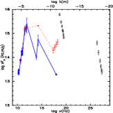
Figure 12: The spectrum of Sgr A* based on all the measurements taken during the first epoch of observations is shown in blue color. This clearly shows that the quiescent flux of Sgr A* peaks in submillimeter wavelength between 0.45 and 2mm, probably near 0.1 mm. The spectrum of Sgr A* is based on measurements at 7mm, 450$\mu$m, 850$\mu$m, 3.6$\mu$m, 1.6$\mu$m and X-rays at 1 keV. The quiescent X-ray and near-IR fluxes are taken from Baganoff et al. (2001), Genzel et al. (2003) and Ghez et al. (2005), though there may not be a true quiescent flux in near-IR wavelengths. All the measurements shown in red color are associated with flaring activity including the X-ray flare with a spectral index of 0.6 detected by XMM (Belanger et al. 2005a). The hard $\gamma$-ray emission from the Galactic center at 1 TeV based on HESS observations (Aharonian et al. 2004) and the high fluxes from INTEGRAL observations are not connected and are only shown by themselves in black color with the corresponding spectral index of 2.2 and 2.06, respectively. The mean flux and the 1-$\sigma$ error are determined from data taken closest to the simultaneous near-IR/X-ray flare.

In order to get a simultaneous spectrum of Sgr A*, we used the data from both epochs of observations. As pointed out earlier, the first epoch data probably represents best the quiescent flux of Sgr A* across its spectrum whereas the flux of Sgr A* includes flare emission during the second epoch. Figure 12 shows power emitted for a given frequency regime as derived from simultaneous measurements from the first epoch (in blue solid line). We have used the mean flux and the corresponding statistical errors of each measurement for each day of observations for the first epoch. Since there were not any near-IR measurements and no X-ray flare activity, we have added the quiescent flux of 2.8 and 1.3 mJy at 1.6 and 3.8 $\mu$m, respectively (Genzel et al. 2003; Ghez et al. 2005) and 20 nJy between 2 and 8 keV (Baganoff et al. 2001) to construct the spectrum shown in Figure 12. For illustrative purposes, the hard $\gamma$-ray flux in the TeV range (Aharonian et al. 2004) is also shown in Figure 12. The F${}_{\nu}\nu$ spectrum peaks at 350 $\mu$m whereas F_ν peaks at 850 $\mu$m in submillimeter domain. The flux at wavelengths between 2 and 3mm as well as between 450 and 850 $\mu$m appear to be constant as the emission drops rapidly toward radio and X-ray wavelengths. The spectrum at near-IR wavelengths is thought to be consistent with optically thin synchrotron emission whereas the emission at radio wavelengths is due to optically thick nonthermal emission.

The spectrum of a flare is also constructed using the flux values in the observing window when the X-ray/near-IR flare took place and is presented in Figure 12 as red dotted line. It is clear that the powers emitted in radio and millimeter wavelengths are generally very similar to each other in both epochs whereas the power is dramatically changed in near-IR and X-ray wavelengths. We also note that the slope of the power generated between X-rays and near-IR wavelengths does not seem to change during the quiescent and flare phase. However, the flare substructures shown in Figure 9 shows clearly that the spectrum between the near-IR to X-ray subflares must be varying. The soft and hard $\gamma$-ray fluxes based on INTEGRAL and HESS (Belanger et al. 2005b; Aharonian et al. 2004) are also included in the plot as black dots. It is clear that F${}_{\nu}\nu$ spectrum at TeV is similar to the observed values at low energies. This plot also shows that the high flux at 20 keV is an upper limit to the flux of Sgr A* because of the contribution from confusing sources within a 13^′ resolution of INTEGRAL.

The simultaneous near-IR and submillimeter flare emission is a natural consequence of optically thin emission. Thus, both near-IR and submillimeter flare emission are nonthermal and no delay is expected between the near-IR and submillimeter flares in this picture. We also compare the quiescent flux of Sgr A* with a flux of 2.8 mJy at 1.6$\mu$m with the minimum flux of about 2.7 Jy at 850$\mu$m detected in our two observing campaigns. The spectral index that is derived is similar to that derived when a simultaneous flare activity took place in these wavelength bands, though there is much uncertainty as to what the quiescent flux of Sgr A* is in near-IR wavelengths. If we use these measurements at face value, this may imply that the quiescent flux of Sgr A* in near-IR and submillimeter could in principle be coupled to each other. The contribution of nonthermal emission to the quiescent flux of Sgr A* at submillimeter wavelength is an observational question that needs to be determined in future study of Sgr A*.

6 Discussion

In the context of accretion and outflow models of Sgr A*, a variety of synchrotron and ICS mechanisms probing parameter space has been invoked to explain the origin of flares from Sgr A*. A detailed analysis of previous models of flaring activity, the acceleration mechanism and their comparison with the simple modeling given here are beyond the scope of this work. Many of these models have considered a broken power law distribution or energy cut-offs for the nonthermal particles, or have made an assumption of thermal relativistic particles to explain the origin of submillimeter emission (e.g., Melia & Falcke 2001; Yuan, Markoff & Falcke 2002; Liu & Melia 2002; Yuan Quataert & Narayan 2003, 2004; Liu, Petrosian & Melia 2004; Atoyan & Dermer (2004); Eckart et al. 2004, 2005; Goldston, Quataert & Tgumenshchev 2005; Liu, Melia, Petrosian 2005; Guillesen et al. 2005) The correlated near-IR and X-ray flaring which we have observed is consistent with a model in which the near-IR synchrotron emission is produced by a transient population of $\sim$GeV electrons in a $\sim$10 G magnetic field of size $\sim 10R_{sch}$. Although ICS and synchrotron mechanisms have been used in numerous models to explain the quiescent and flare emission from Sgr A* since the first discovery of X-ray flare was reported (e.g., Baganoff 2001), the simple model of X-ray, near-IR and submillimeter emission discussed here is different in that the X-ray flux is produced by a roughly equal mix of (a) near-IR photons that are up-scattered by the 50 MeV particles responsible for the quiescent submillimeter emission from Sgr A*, and/or (b) submillimeter photons up-scattered from the GeV electron population responsible for the near-IR flares. Thus, the degeneracy in these two possible mechanisms can not be removed in this simple model and obviously a more detailed analysis is needed. In addition, we predict that the lack of a correlation between near-IR and X-ray flare emission can be explained by the variation of spectral index and/or the magnetic fields. The variation of these parameters in the context of the stochastic acceleration model of flaring events has also been explored recently (Liu, Melia and Petrosian 2005; Gillesen et al. 2005).

The similar durations of the submillimeter and near-IR flares imply that the transient population of relativistic electrons loses energy by a dynamical mechanism such as adiabatic expansion rather than frequency-dependent processes such as synchrotron cooling. The dynamical time scale 1/$\Omega$ (where $\Omega$ is the rotational angular frequency) is the natural expansion time scale of a build up of pressure. This is because vertical hydrostatic equilibrium for the disc at a given radius is the same as the dynamical time scale. In other words, the time for a sound wave to run vertically across the disc, h/c_s = 1/$\Omega$. The 30–40 minute time scale can then be identified with the accretion disk’s orbital period at the location of the emission region, yielding an estimate of $3.1-3.8\,R_{sch}$ for the disc radius where the flaring is taking place. This estimate has assumed that the black hole is non-rotating (a/M = 0). Thus, the orbiting gas corresponding to this period has a radius of 3.3 R_sch which is greater than the size of the last stable orbit. Assuming that the significant power at 33-minute time scale is real, it confirms our source size assumption in the simple ICS model for the X-ray emission. If this general picture is correct, then more detailed hot-spot modeling of the emission from the accreting gas may be able to abstract the black hole mass and spin from spot images and light curves of the observed flux and polarization (Bromley, Melia & Liu 2001; Melia et al. 2001; Broderick and Loeb 2005a,b).

Assuming the 33-minute duration of most of the near-IR flares is real, this time scale is also comparable with the synchrotron loss time of the near-IR-emitting ($\sim 1$ GeV) electrons in a 10 G field. This time scale is also of the same order as the inferred dynamical time scale in the emitting region. This is not surprising considering that if particles are accelerated in a short initial burst and are confined to a blob that subsequently expands on a dynamical time scale, the characteristic age of the particles is just the expansion time scale. The duration of submillimeter flare presented here appears to be slightly longer (roughly one hour), than the duration of near-IR flares (about 20–40minutes) (see also Eckart et al. 2005). This is consistent with the picture that the blob size in the context of an outflow from Sgr A* is more compact than in that at submillimeter wavelength. The spectrum of energetic particles should then steepen above the energy for which the synchrotron loss time is shorter than the age of the particles, i.e., in excess of a few GeV. This is consistent with a steepening of the flare spectrum at wavelengths shorter than a micron.

The picture described above implies that flare activity drives mass-loss from the disk surface. The near-IR emission is optically thin, so we can estimate the mass of relativistic particles in a blob (assuming equal numbers of protons and electrons) and the time scale between blob ejections. If the typical duration of a flare is 30 minutes and the flares are occurring 40% of the time, the time scale between flare is estimated to be $\sim$75 minutes. Assuming equipartition of particles and field with an assumed magnetic field of 11G and using the spectral index of near-IR flare $\alpha=0.6$ identical to its X-ray counterpart, the density of relativistic electrons is then estimated to be n${}_{e}=3.5\times 10^{2}$ cm^-3 (The steepening of the spectral index value to 1 increases particles density to 4.6$\times 10^{2}$ cm^-3.) The volume of the emitting region is estimated to be $785R_{Sch}^{3}$. The mass of a blob is then $\sim 5\times 10^{15}$ g if we use a typical flux of 3.9 mJy at 1.6$\mu$m. The time-averaged mass-loss rate is estimated to be $\sim 2\times 10^{-12}\hbox{$M_{\odot}$}yr^{-1}$. If thermal gas is also present at a temperature of T$\sim 5\times 10^{9}$ K with the same energy density as the field and relativistic particles, the total mass-loss due to thermal and nonthermal particles increases to $\sim 1.3\times 10^{-8}$ $M_{\odot}$yr^-1 (this estimate would increase by a factor of 2.5 if we use a flux of 9.3 mJy for a typical flare). Using a temperature of 10¹¹ K, this estimate is reduced by a factor of 20. It is clear from these estimates that the mass-loss rate is much less than the Bondi accretion rate based on X-ray measurements (Baganoff et al. 2003). Similarly, recent rotation measure polarization measurements at submillimeter wavelength place a constraint on the accretion rate ranging between 10^-6 and 10^-9 $M_{\odot}$yr^-1 (Marrone et al. 2005).

7 Summary

We have presented the results of an extensive study of the correlation of flare emission from Sgr A* in several different bands. On the observational side, we have reported the detection of several near-IR flares, two of which showed X-ray and submillimeter counterparts. The flare emission in submillimeter wavelength and its apparent simultaneity with a near-IR flare are both shown for the fist time. Also, remarkable substructures in X-ray and near-IR light curves are noted suggesting that both flares are simultaneous with no time delays. What is clear from the correlation analysis of near-IR data is that relativistic electrons responsible for near-IR emission are being accelerated for a high fraction of the time (30-40%) having a wide range of power law indices. This is supported by the ratio of flare emission in near-IR to X-rays. In addition, the near-IR data shows a marginal detection of periodicity on a time scale of $\sim$32 minutes. Theoretically, we have used a simple ICS model to explain the origin of X-ray and soft $\gamma$-ray emission. The mechanism to up-scatter the seed submillimter photons by the GeV electrons which produce near-IR synchrotron emission has been used to explain the origin of simultaneous near-IR and X-ray flares. We also explained that the submillimeter flare emission is due to synchrotron emission with relativistic particle energies extending down to $\sim$50 MeV. Lastly, the equal flare time scale in submillimeter and near-IR wavelengths implies that the burst of emission expands and cools on a dynamical time scale before they leave Sgr A*. We suspect that the simple outflow picture presented here shows some of the characteristics that may take place in micro-quasars such as GRS 1915+105 (e.g., Mirabel and Rodriguez 1999).

Acknowledgments: We thank J. Mauerhan and M. Morris for providing us with an algorithm to generate the power spectrum of noise and L. Kirby, J. Bird, and M. Halpern for assistance with the CSO observations. We also thank A. Miyazaki for providing us the NMA data prior publication.

Figure 2: (a) The light curves of Sgr A* and star S0-3 in the NICMOS F160W band, using apertures of four pixels in diameter. The data for Sgr A* clearly show flare activity, while the signal from S0-3 is quite constant (top panel). (b) Near-IR light curves of Sgr A* using four-pixel diameter apertures are shown in six observing windows. Flare activity has been detected in three windows in all three bands. The fluxes shown are the observed fluxes in each band, uncorrected for reddening. Measurement uncertainties are $\sim$0.002 mJy in the 1.60 $\mu$m band and $\sim$0.005 mJy in the 1.87 and 1.90 $\mu$m bands (bottom panel).

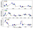
Figure 3: (a) Light curves of Sgr A* in three different observing time windows during which near-IR flare activity took place. The blue, green, and red points represent the 1.60, 1.87, and 1.90 $\mu$m bands, respectively. The broadband 1.60 $\mu$m data points are sampled every 32 sec, whereas the narrow-band 1.87 and 1.90 $\mu$m data are averages of six 32 sec data points, in order to get similar S/N ratio in the three bands. (b) This is a plot showing the simultaneous 2-Gaussian fit to the histogram of both the noise and the flare emission at 1.6$\mu$m. The dotted lines are the individual Gaussians, while the thick dashed line is the sum of the two.

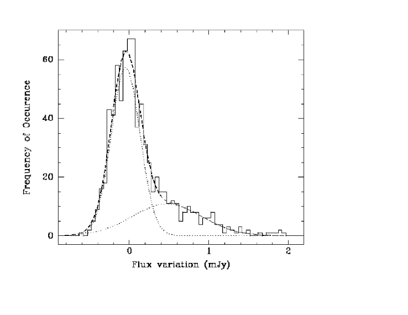
Figure 3:

Figure 6: The complex gain of the calibrators as a function of time and the corresponding light curves of Sgr A* based on VLA and ATCA observations at 7mm and 1.2cm are shown in the top (a) and bottom panels (b), respectively.

References

- Aharonian, F. et al. 2004, A&A, 425, L13
- (1) Aschenbach, B., Grosso, N., Porquet, D. &Predehl, P. 2004, A&A, 417, 71
- (2) Aschenbach, B. 2005, In “Growing black holes: accretion in a cosmological context”, Proceedings of the MPA/ESO/MPE/USM Joint Astronomy Conference held at Garching, Germany, 21-25 June 2004. eds: A. Merloni, S. Nayakshin, R. A. Sunyaev ESO astrophysics symposia. Berlin: Springer, ISBN 3-540-25275-4, ISBN 978-3-540-25275-7, 2005, p. 302 - 303 (arXiv:astro-ph/0410328)
- (3) Agol, E. 2000, ApJ, 538, L121
- (4) Aitken, , D.K., Greaves, J., Chrysostomou, A., Jenness, T., Holland, W., Hough, J.H., Pierce-Price, D. & Richer, J. 2000, ApJ, 534, L173
- (5) Atoyan, A. & Dermer, C. D. 2004, ApJ, 617, L123
- (6) Baars, J.W.M., Martin, R.N., Mangum, J.G., McMullin, J.P. & Peters, W.L. 1999, PASP, 111, 627
- (7) Balick, A. & Brown, R.L. 1974, ApJ, 194,265
- (8) Baganoff, F.K., Maeda, Y., Morris, M., Bautz, M.W., Brandt, W.N. et al. 2003, ApJ, 591, 891
- (9) Baganoff, F. K., Bautz, M.W., Brandt, W.N., Chartas, G., Feigelson, E.D. et al. 2001, Nature 413, 45
- (10) Belanger, G., Goldwurm, A., Melia, F., Yusef-Zadeh, F., Ferrando, P. et al. 2005a, ApJ, (in press)
- (11) Belanger, G., Goldwurm, A., Renaud, M., Terrier, R., Melia, F., Lund, N., Paul, J., Skinner, G. & Yusef-Zadeh, F. 2005b, ApJ, in press
- (12) Bower, G., Roberts, D., Yusef-Zadeh, F., Becker, D.C., Cotton, W.D., Lang, C.C. & Lithwick, Y. 2005, ApJ, in press
- (13) Bower, G.C., Falke, H., Sault, R.J. & Backer, D.C. 2002, ApJ 571, 843
- (14) Broderick A. E., Loeb, A. 2005a, ApJ submitted (astro-ph/0508386)
- (15) Broderick A. E., Loeb, A. 2005b MNRAS submitted (astro-ph/0509237)
- (16) Bromley, B.C., Melia, F. & Liu, S. 2001, ApJ, 555, L83
- (17) DePoy, D.L., Pepper, J., Pogge, R.W., Stutz, A., Pinsonneault, M. & Sellgren, K. 2004, ApJ, 617, 1127
- (18) Dowell, C.D., Kirby, L., Novak, G. & Yusef-Zadeh, F. 2004, BAAS, 205, 3205
- (19) Eckart, A., Baganoff, F. K., Morris, M., Bautz, M.W., Brandt, W.N. et al. 2004, A&A, 427, 1
- (20) Eckart, A. et al. 2005, in preparation
- (21) Eisenhauer, F., Genzel, R., Alexander, T., Abuter, R., Paumard, T., Ott, T., Gilbert, A., Gillessen, S., Horrobin, M., Trippe, S. et al. 2005, ApJ, 628, 246
- (22) Genzel, R., Schödel, R., Ott, T., Eckart, A., Alexander, T., Lacombe, F., Rouan, D., Aschenbach, B. et al. 2003, Nature, 425, 6961, 934
- (23) Ghez, A. M., Wright, S. A., Matthews, K., Thompson, D., Le Mignant, D., Tanner, A., Hornstein, S. D., Morris, M., Becklin, E. E. & Soifer, B. T. 2004, ApJ, 601, L159
- (24) Ghez, A. M., Hornstein, S.D., Lu, J., Bouchez, A., Le Mignant, D. et al. 2005, ApJ, 635 (in press)
- (25) Gillessen, S., Eisenhauer, F., Quataert, E., Genzel, R., Paumard, T., Trippe, Ott, T. et al. 2005, ApJ, submitted (astro-ph/0511302)
- (26) Goldston, J., Quataert, E. & Tgumenschchev, I.V. 2005, ApJ, 621, 785
- (27) Goldwurm, A., Brion, E., Goldoni, P., Ferrando, P., Daigne, F., Decourchelle, A., Warwick, R. S. & Predehl, P. 2003, ApJ, 584, 751
- (28) Herrnstein, R.M., Zhao, J.-H., Bower, G.C. & Goss, W. M. 2004, AJ, 127, 3399
- (29) Liu, S. & Melia, F. 2001, ApJ, 561, L77
- (30) Liu, S. & Melia, F. 2002, ApJ, 566, L77
- (31) Liu, S., Petrosian, V. & Melia, F. 2004, ApJ, 611, L101
- (32) Liu, S., Melia, F. & Petrosian, V. 2005, ApJ, submitted (astro-ph/0506151)
- (33) Macquart, J.-P. & Bower, G.C., 2005, ApJ, submitted.
- (34) Markoff, S. 2005, ApJ, 618, L103
- (35) Marrone, D.P., Moran, J., Zhao, J.-H. &Rao, R. 2005, ApJ, in press (astro-ph/0511653)
- (36) Mauerhan, J.C., Morris, M., Walter, F. & Baganoff, F. 2005, ApJ, 623, L25
- (37) Melia, F., Liu, S. & Coker, R. 2000, ApJ, 545, L117
- (38) Melia, F., Bromley, B., Liu, S. & Walker, C.K. 2001, ApJ, 554, L37
- (39) Melia, F., & Falcke, H. 2001, ARAA, 39, 309
- (40) Mirabel, I.F. & Rodriguez, L.F. 1999, 37, 409
- (41) Miyazaki, A., Tsutsumi, T. & Tsuboi, M. 2004, ApJ 611, L97
- (42) Moneti, A., Stolovy, S., Blommaert, J.A.D.L., Figer, D. F. & Najarro, F. 2001, A&A, 366, 106
- (43) Muno, M.P., Lu, J.R., Baganoff, F.K., Brandt, W.N., Garmire, G.P., Ghez, A. M., Hornstein, S.D. & Morris, M.R. 2005, ApJ, in press
- (44) Porquet, D., Predehl, P., Aschenbach, B., Grosso, N., Goldwurm, A., Goldoni, P., Warwick, R.S. & Decourchelle, A. 2003, A&A, 407, L17
- (45) Porquet, D., Grosso, N., Belanger, G., Goldwurm, A., Yusef-Zadeh, F., Warwick, R. S. & Predehl, P. 2005, A&A, in press
- (46) Roberts et al. 2005, in preparation
- (47) Scargle, J.D. 1982, ApJ, 263, 835
- (48) Schödel, R., Ott, T., Genzel, R., Hofmann, R., Lehnert, M., Eckart, A., Mouawad, N., Alexander, T., Reid, M. J. & Lenzen R. 2002, Nature, 419, 694
- (49) Stolovy, S.R., McCarthy, D.W., Melia, F., Rieke, G., Rieke, M. J. & Yusef-Zadeh, F. 1999, in The Central Parsecs of the Galaxy, ASP Conference Series, Vol. 186. Edited by H. Falcke, A. Cotera, W. J. Duschl, F. Melia, and M. J. Rieke. ISBN: 1-58381-012-9, p39
- (50) Timmer, J. & König, M. 1995, A&A, 300, 707
- (51) Tsutsumi, T., Miyazaki, A. & Tsuboi, M. 2005, AJ (submitted)
- (52) Yuan, F., Markoff, S., & Falcke, H. 2002, A&A, 854, 383
- (53) Yuan, F., Quataert, E. & Narayan, R. 2003, ApJ, 598, 301
- (54) Yuan, F., Quataert, E. & Narayan, R. 2004, ApJ, 606, 894
- (55) Zhao, J.-H., Young, K.H., Hernstein, R.M. et al. 2003, ApJ, 586, L29
- (56)