A recalibration of optical photometry: Tycho-2, Strömgren, and Johnson systems

Abstract

I use high-quality HST spectrophotometry to analyze the calibration of three popular optical photometry systems: Tycho-2 $B_{\rm T}$$V_{\rm T}$, Strömgren $uvby$, and Johnson $UBV$. For Tycho-2, I revisit the analysis of Maíz Apellániz (2005a) to include the new recalibration of grating/aperture corrections, vignetting, and charge transfer inefficiency effects produced by the STIS group and to consider the consequences of both random and systematic uncertainties. The new results reaffirm the good quality of both the Tycho-2 photometry and the HST spectrophotometry, but yield a slightly different value for ZP${}_{B_{\rm T}-V_{\rm T}}$ of $0.033\pm 0.001$ (random) $\pm 0.005$ (systematic) magnitudes. For the Strömgren $v$, $b$, and $y$ filters I find that the published sensitivity curves are consistent with the available photometry and spectrophotometry and I derive new values for the associated ZP_b-y and ZP${}_{m_{1}}$. The same conclusion is drawn for the Johnson $B$ and $V$ filters and the associated ZP_B-V. The situation is different for the Strömgren $u$ and the Johnson $U$ filters. There I find that the published sensitivity curves yield results that are inconsistent with the available photometry and spectrophotometry, likely caused by an incorrect treatment of atmospheric effects in the short-wavelength end. I reanalyze the data to produce new average sensitivity curves for those two filters and new values for ZP${}_{c_{1}}$ and ZP_U-B. The new computation of synthetic $U-B$ and $B-V$ colors uses a single $B$ sensitivity curve, which eliminates the previous unphysical existence of different definitions for each color. Finally, I find that if one uses values from the literature where uncertainties are not given, reasonable estimates for these are $1-2$% for Strömgren $b-y$, $m_{1}$, and $c_{1}$ and $2-3$% for Johnson $B-V$ and $U-B$. The use of the results in this article should lead to a significant reduction of systematic errors when comparing synthetic photometry models with real colors and indices.

1 Introduction

The data explosion of the last decade has produced large quantities of photometric measurements, either from dedicated ground-based projects (e.g. 2MASS, Skrutskie et al. 1997), compilations from different sources (e.g. GCPD, Mermilliod et al. 1997), or dedicated space-based missions (e.g. Hipparcos, ESA 1997). The future promises an expansion of the phenomenon with the final publication of data from projects such as the Sloan Digital Sky Survey (York et al., 2000) or GALEX (Bianchi et al., 1999) and new missions such as GAIA (Mignard, 2005).

The photometry from space-based missions is obtained with a fixed instrumental setup, does not suffer from perturbing atmospheric effects, and can be supported by a dedicated calibration program. On the other hand, observing from space also has its negative effects (e.g. the existence of Charge Transfer Inefficiency, or CTI, in CCD detectors due to radiation damage, Kimble et al. 2000) but, overall, the available data from recent space-based missions have very good photometric characteristics. The dedicated ground-based projects of the last decade also benefit from the uniformity of the instrumental setup, observing site, and reduction techniques and, though affected by the atmosphere, they can implement extensive calibration programs and quality control mechanisms to ensure the stability of the obtained data (see, e.g. Cohen et al. 2003, Smith et al. 2002). Large dedicated photometric projects (either space- or ground-based) also benefit from the volume of the datasets and their coverage of a significant part of the sky (or all of it), which allow for statistical tests to detect possible systematic effects in the data.

The situation is quite different for compilations of older ground-based data (see, e.g. Lanz 1986; Hauck & Mermilliod 1998), which typically include tens or hundreds of studies, each one of them with tens or hundreds of objects. The large number of sources implies different detectors, filters, observatories, and reduction techniques, which undoubtedly introduce a scatter in the data and, quite possibly, systematic errors (see Stetson 2005 and references therein for a detailed discussion on the problems associated with the reduction of ground-based photometry). Furthermore, in many cases the photometry obtained in the “standard” systems (e.g. Johnson or Strömgren) was established using equipment with lower precision than the one available today and using standard stars with a limited range of colors. Therefore, it is possible that some systematic errors may have been introduced from the very beginning, thus complicating a recalibration of the data. Those effects led Bessell et al. (1998) to conclude that (a) standard systems may not represent any real linear system and (b) we should not be reluctant to include ad-hoc corrections of a few percent to achieve an agreement between the observed and the synthetic photometry in such systems. This rather pessimistic view may lead somebody to ask oneself why should we bother about the recalibration of photometric systems half-a-century old. The answer to that question is that many of the current calibrations are eventually tied up to those standard systems, as evidenced by the fact that the most common way to simply characterize the photometric properties of an object in a research proposal is to give its Johnson $V$ magnitude and $B-V$ color. If we renounce to calibrate standard systems accurately we are condemned to have systematic errors propagating down our reduction procedure.

In this paper I take a more optimistic view of the problem by stating two points. In the first place, even though it is true that some standard systems cannot be strictly characterized by a sensitivity (or throughput) curve and a zero point for each magnitude and/or color, it is also true that does not stop us from trying to derive the corresponding function and value that minimize the scatter of the data. In the second place, some of the calibration problems encountered in the past may have been due not to the photometry itself but to the data used to calibrate it, e.g. systematic errors in the measured spectrophotometry or in the assumed stellar model parameters. Therefore, the use of more modern calibration data may increase the accuracy. In other words, I believe it is possible to eliminate at least some of the systematic errors in the photometric calibration and to significantly lower the uncertainties in the zero points.

In paper I (Maíz Apellániz, 2005a), I used HST spectrophotometry to analyze Tycho-2 photometry in order to check the accuracy of its published sensitivity curves and to calculate the zero points. In this paper, I start by revisiting those data and then I use similar techniques to analyze the two most common optical standard systems: Strömgren $uvby$ and Johnson $UBV$. In all cases, Vega will be used as the reference spectrum to calculate magnitudes, colors, and indices (see Appendices).

2 Spectrophotometry

A straightforward method to test the sensitivity curves and to calculate the zero points of filter systems is to observe a number of stars with well-characterized and sufficiently different spectral energy distributions (SEDs) and to compare the measured photometric magnitudes/colors/indices with those derived from synthetic photometry. If the sensitivity curves are correct, a plot of the difference between the measured and synthetic values as a function of color or magnitude should yield a straight line with zero slope and an intercept equal to the zero point (see Appendices). If a slope is present in such a plot, then the assumed sensitivity curves may be incorrect due to e.g. an inaccurate characterization of atmospheric effects (which enter in the sensitivity curve for ground-based observations in the reduction process to extrapolate to zero air masses) or an imprecise calibration of the detector. Of course, it is also possible that the cause of a non-zero slope lies in the SED library, and not in the photometry itself. Therefore, a necessary preliminary step in the process is to ensure that the SEDs are as accurate as possible.

The Space Telescope Imaging Spectrograph (STIS) onboard Hubble Space Telescope (HST) was able to provide during its seven years of operation the most accurate to-date spectrophotometry in the 1 150-10 200 Å range. The accuracy of its absolute flux calibration in the $V$ band is 1.1%, of which 0.7% corresponds to the value of the absolute flux of Vega at the $V$ band (Mégessier, 1995) and 0.8% to uncertainties in the photometry (Bohlin, 2000; Bohlin & Gilliland, 2004b). On the other hand, the accuracy of its relative flux calibration with respect to the $V$ band depends on the uncertainty of the temperature of the three white dwarfs used as primary calibrators. This can be as high as 1-3% in the FUV but in the optical it is significantly lower due to the degeneracy of the spectral slopes at high temperatures. The accuracy of an individual STIS spectrophotometric observation is also limited by the instrument repeatability, which is 0.2-0.4% for the wavelength range in which I am interested in this paper (Bohlin, 2000; Bohlin & Gilliland, 2004a).

In this article I will use the same two STIS samples as in Paper I: the Next Generation Spectral Library (NGSL; Gregg et al. 2004) and the Bohlin sample (Bohlin et al., 2001; Bohlin & Gilliland, 2004a). The reader is referred to Paper I for details. The NGSL sample is large ($\gtrsim 250$ non-variable stars), is made up of relatively bright stars ($V$ between 2.5 and 11.5), and includes a large variety of SED types (sampling diverse temperatures, metallicities, and gravities), but was obtained with a STIS configuration (52X0.2 long slit at the E1 detector position and reading only a subarray of the CCD) which introduces some complications in the calibration. The Bohlin sample is smaller (19 stars), consists of dimmer objects (only 2 are brighter than $V=9$, implying that only some of the stars have reliable multicolor photometry available in the standard systems), and is made up mostly of early-type stars (only 5 stars have $\mbox{$B-V$}>0.0$). The latter sample, however, uses the preferred STIS setup for absolute photometry (52X2 long slit at the center of the detector and reading the full CCD) and, in most cases, have repeated observations, thus allowing for a more straightforward calibration.

Some of the calibration issues regarding the NGSL sample were discussed and dealt with in Paper I. Since that article was published, the STIS group (Proffitt, 2005) has identified a number of issues that prompted me to reprocess the data in order to improve the calibration. On the first place, it was discovered that the effective throughput as a function of wavelength for a given long slit (e.g. 52X2 or 52X0.2) was not the same for all STIS gratings. This effect has been corrected in the STIS pipeline by introducing a grating/aperture correction table and making the appropriate changes in the calstis software. Second, a new L-flat that incorporates the effects of vignetting and that should improve the flux calibration at the E1 detector position has been calculated. Finally, an error in the algorithm that calculates the CTI for subarrays has been fixed. All of the above issues have no effect on the broadband colors of the Bohlin sample but can produce changes at the 1-2% level for the broadband colors of the NGSL sample. For that reason, before proceeding with an analysis of the Strömgren and Johnson systems, I study the effects of the new calibration on the paper I results for Tycho-2 photometry.

3 Tycho-2 $B_{\rm T}$$V_{\rm T}$

As previously mentioned, the purpose of paper I was to test the published sensitivity curves for the two Tycho-2 filters, $B_{\rm T}$ and $V_{\rm T}$ (Bessell, 2000), and to calculate their zero points. I found out in that paper that the sensitivity curves were indeed correct and derived a value of $\mbox{ZP${}_{B_{\rm T}}$}=0.078\pm 0.009$ from the Bohlin sample and of $\mbox{ZP${}_{B_{\rm T}-V_{\rm T}}$}=0.020\pm 0.001$ from the NGSL sample. The uncertainties quoted there are only the random ones and were derived by inverse variance weighting from the photometry. The new calibration of the NGSL data can (and indeed does, as we will see next) affect the value for ZP${}_{B_{\rm T}-V_{\rm T}}$ but not that of ZP${}_{B_{\rm T}}$, which was derived from the Bohlin sample.

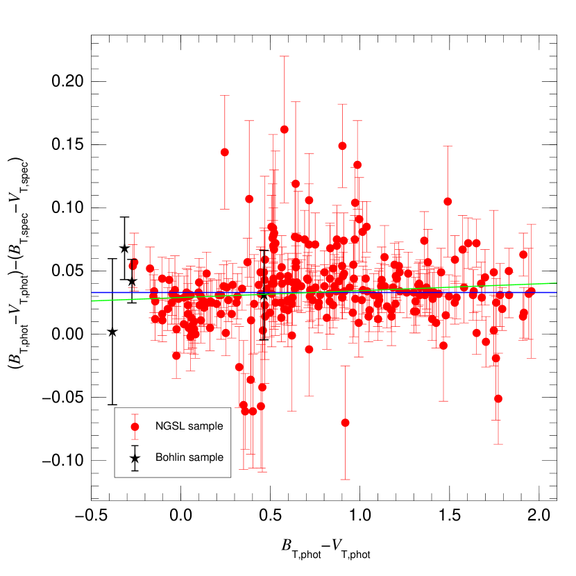
Figure 1: Comparison between photometric and spectrophotometric $B_{\rm T}-V_{\rm T}$ colors as a function of photometric $B_{\rm T}-V_{\rm T}$ for the NGSL + Bohlin samples. The error bars represent the photometric uncertainties and the horizontal blue line marks the proposed ZP${}_{B_{\rm T}-V_{\rm T}}$. The green line shows the result of a weighted linear fit to the data.

I have reprocessed the NGSL data through calstis and retained only the non-variable stars with a 5 600 Å jump (the point where the G430L and G750L gratings overlap) of less than 3% and with uncertainties in the measured $B_{\rm T}$ and $V_{\rm T}$ magnitudes smaller than 0.06 mag. This left 255 objects (as opposed to 256 in Paper I) for which the synthetic (or spectrophotometric) $B_{\rm T}$ and $V_{\rm T}$ magnitudes were computed. I show the difference between the photometric values (from the Tycho-2 catalog) and spectrophotometric values (from the STIS spectra) of $B_{\rm T}-V_{\rm T}$ in Fig. 1, which is the equivalent to Fig. 2 in Paper I.

Figure 2: Histograms for the comparison between photometric and spectrophotometric $B_{\rm T}-V_{\rm T}$ colors for the NGSL sample. (left) Regular histogram. (right) Histogram for the data shifted by the proposed ZP${}_{B_{\rm T}-V_{\rm T}}$ and normalized by the individual uncertainties. A Gaussian distribution with $\mu=0$ and $\sigma=1$ is overplotted for comparison.

The main conclusion remains the same as in the previous paper: there is a very good correspondence between the photometric and spectrophotometric $B_{\rm T}-V_{\rm T}$ colors, as evidenced by the nearly-flat distribution of points in Fig. 1. The normalized histogram in Fig. 2 also corroborates that assertion: the residuals appear to be symmetrically distributed around the zero point and the standard deviation of the histogram is 1.04, as in Paper I. Here I have also performed an additional test by fitting a weighted straight line to the data in Fig. 2, which is shown in green. The slope of the fit is nearly flat but not exactly so: $0.005\pm 0.002$. This implies that either the Tycho-2 sensitivities or the calibration of the NGSL data are not perfect. However, the effect is very small, since the deviations at the edges of the used color spectrum (which correspond to low-reddening O and M stars, respectively) amount to only $\pm 0.006$ magnitudes, which is 1/3 of the best individual photometric uncertainty for the colors in our sample. Also, $0.002/0.005=2.5$, i.e. the slope is only 2.5 sigmas away from zero. Therefore, I do not consider necessary to derive new sensitivity curves for the Tycho-2 filters. Instead, this effect will be included in the error analysis below as a systematic uncertainty.

The new value I obtain for the $B_{\rm T}-V_{\rm T}$ zero point using inverse variance weighting is $\mbox{ZP${}_{B_{\rm T}-V_{\rm T}}$}=0.033\pm 0.001$, which is significantly larger than the value derived in Paper I ($0.020\pm 0.001$). The 1.3% difference between the two is within the expected range of the changes introduced in the new STIS calibration (Proffitt, 2005). It is interesting to note that if I only use the four Bohlin stars in Fig. 1 to calculate ZP${}_{B_{\rm T}-V_{\rm T}}$, I obtain a value of $0.046\pm 0.013$, which is at a distance of 1 sigma from the value proposed here but 2 sigmas away from the previous one. Those values are consistent with an improvement in the new STIS calibration. The uncertainty of 0.001 is a purely random one but, as we have seen before, there are also systematic effects present. The slope to the fit described in the previous paragraph translates into a 1-sigma uncertainty of 0.003 magnitudes. Furthermore, the uncertainty of 3 000 K in the temperature of the white dwarf calibrators quoted by Bohlin & Gilliland (2004a) translates into an additional (systematic) uncertainty of 0.004 magnitudes, which was calculated using synthetic photometry of Kurucz models. Therefore, the proposed final value is $\mbox{ZP${}_{B_{\rm T}-V_{\rm T}}$}=0.033\pm 0.001$ (random) $\pm 0.005$ (systematic) magnitudes.

As for the absolute calibration of Tycho-2 photometry, I defer its analysis until the Johnson $UBV$ photometry is analyzed.

4 Strömgren $uvby$

4.1 Description and sample selection

The Strömgren standard system (Matsushima, 1969) has been the most commonly used intermediate-band photometric optical system in the last 40 years. It consists of 4 filters in the 3 000-6 000 Å range, $u$, $v$, $b$, and $y$ and the quantities that are presented in most works are:

$$b-y$$ (1)

$$m_{1} = v-2b+y$$ (2)

$$c_{1} = u-2v+b$$ (3)

$b-y$ is a color similar (but not identical) to Johnson $B-V$ or to Tycho-2 $B_{\rm T}-V_{\rm T}$, $m_{1}$ is an index that is most sensitive to the metallicity of a star, and $c_{1}$ is an index that measures the strength of the Balmer jump (Strömgren, 1966). Hauck & Mermilliod (1998) have published a catalog of photometric measurements in the Strömgren system compiled from photoelectric data in the literature. In its current (summer 2005) version, available from the General Catalogue of Photometric Data (GCPD), it contains 66 135 stars from 572 different sources.

I want to test whether the Matsushima (1969) sensitivity curves are consistent with the photometry in the literature (in the sense of not having strong color terms when compared with the STIS spectrophotometry) and to calculate the corresponding zero points for $b-y$, $m_{1}$, and $c_{1}$. Note that the Strömgren GCPD data includes only one color and two indices, but not magnitudes (though Johnson $V$ is usually also given in many cases), so, as opposed to the Tycho-2 or Johnson cases, I only have to deal here with color/index zero points. We also need to consider that, as opposed to the Tycho-2 case, some of the scatter in the published photometric data is unavoidable due to the diversity of the sources. Therefore, our aims should be to obtain mean color/index values for the stars in our samples that are representative of that diversity and to measure the intrinsic scatter. On the other hand, I should not include in the sample highly discrepant values that are caused by incorrect reductions or misidentifications because that would misrepresent the scatter that is really unavoidable and may introduce biases in the interpretation of correct data. The elaboration of a photometric sample that is appropriate for a comparison with STIS spectrophotometry must allow both of those principles to be followed by selecting stars for which there are enough data to discriminate which values to include. With those ideas in mind, I followed these steps to create the Strömgren photometric sample:

1. I started by searching in the GCPD for the original Strömgren photometry (i.e. not the mean values) for all non-variable stars in the NGSL sample and for all stars in the Bohlin sample. As I did for the Tycho-2 case, for the NGSL sample only those stars with a 5 600 Å jump in the spectrophotometry of less than 3% were included.

2. I calculated a weighted mean and a dispersion for $b-y$, $m_{1}$, and $c_{1}$ for each star, which are taken to be the first estimate for the value and random uncertainty, respectively, for each of those color/indices.

3. Highly discrepant individual data points (those more than 3 sigmas from the mean) were excluded and the mean and dispersion recalculated for $b-y$, $m_{1}$, and $c_{1}$ for each star.

4. Only stars that had (a) at least three data points for each of $b-y$, $m_{1}$, and $c_{1}$ after the previous step and (b) random uncertainties of less than 0.035 magnitudes were kept in our sample and the rest were excluded. This step provides a more meaningful value to the statistical weight that will be derived from the random uncertainty (i.e. it eliminates values that are likely to be biased or of lower quality).

5. For the stars with Tycho-2 photometry, I plotted $b-y$ vs. $B_{\rm T}-V_{\rm T}$ (which should follow a quite tight correlation) and discarded the discrepant cases.

6. For each of the three indices, the remaining stars were divided into two groups: (a) those with 6 or more data points and (b) those with 3 to 5 data points. For the first group, those objects that had an uncertainty less than a critical value $\varepsilon_{X}$ (where $X$ = $b-y$, $m_{1}$, or $c_{1}$) had that uncertainty replaced by $\varepsilon_{X}$. For the second group, the same procedure was repeated but using $2\varepsilon_{X}$ as the replacement in order to account for the lower statistical weight that should be assigned to stars with a smaller number of data points. There are two reasons for doing this. First, I avoid giving excessive statistical weights to those cases where due to roundoff or special circumstances (e.g. most data points coming from an identical instrumental setup and observing conditions) the dispersion of the data points is too low. Second, I can vary $\varepsilon_{X}$ iteratively in order to get an accurate measurement of the true intrinsic scatter by demanding that, once a zero point has been calculated, the difference between the photometric and spectrophotometric values has a reduced $\chi^{2}$ of 1.0 (or, alternatively, since the number of stars in our sample is large, that the normalized histogram $(X_{\rm phot}-X_{\rm spec})/\sigma_{X}$ has a mean of zero and a standard deviation of one). The initial values of $\varepsilon_{b-y}$, $\varepsilon_{m_{1}}$, and $\varepsilon_{c_{1}}$ were obtained from Hauck & Mermilliod (1998).

After the selection process was completed, I ended up with a total of 104 stars, 100 from the NGSL sample and 4 from the Bohlin sample. In the next subsections I describe the results for $b-y$, $m_{1}$, and $c_{1}$, respectively.

4.2 $b-y$

The results for $b-y$ can be seen in Fig. 3, where I have represented the difference between the photometric and spectrophotometric values as a function of the photometric ones, in a manner analogous to that of the previous section for $B_{\rm T}-V_{\rm T}$. $\varepsilon_{b-y}$ was iteratively determined to be 0.008 mag using the criterion stated in the previous subsection. The data does not manifest any significant trend with color and this shows in the slope of the weighted linear fit, which is $-0.004\pm 0.005$ mag (less than 1 sigma away from zero). Also, the slope of the fit has the opposite sign to the one I found for $B_{\rm T}-V_{\rm T}$, suggesting that the (small) discrepancies lie in the photometry, not in the STIS spectra. Furthermore, no obvious different trend is seen between the objects in the NGSL and Bohlin samples. Therefore, I can conclude that the Matsushima (1969) sensitivity curves for $b$ and $y$ provide an accurate description for those filters.

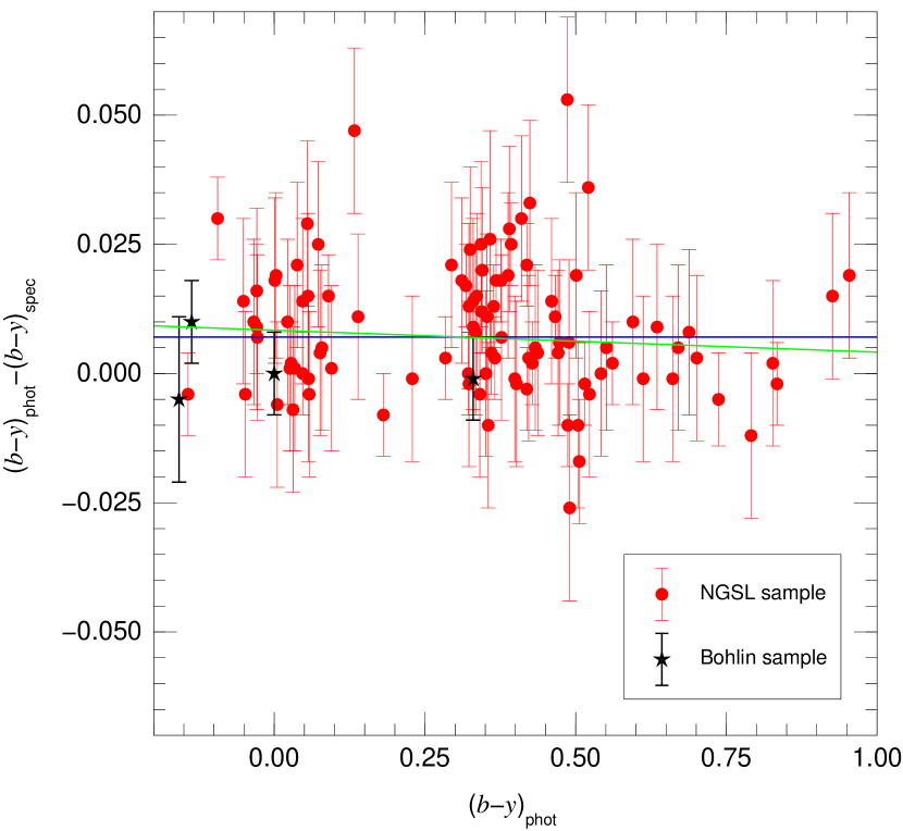
Figure 3: Comparison between photometric and spectrophotometric $b-y$ colors as a function of photometric $b-y$ for the NGSL + Bohlin samples. The error bars represent the photometric uncertainties and the horizontal blue line marks the proposed ZP_b-y. The green line shows the result of a weighted linear fit to the data.

As I did for $B_{\rm T}-V_{\rm T}$, the zero point was calculated using inverse variance weighting to obtain $\mbox{ZP${}_{b-y}$}=0.007\pm 0.001$. For the systematic uncertainties there are two sources, which I can calculate using the same techniques as for $B_{\rm T}-V_{\rm T}$. From the weighted linear fit of the data there is a 1-sigma uncertainty of 0.001 mag and from the uncertainty of 3 000 K in the white dwarf calibration I get 0.003 mag. Combining them in quadrature I obtain $\mbox{ZP${}_{b-y}$}=0.007\pm 0.001$ (random) $\pm 0.003$ (systematic) magnitudes.

4.3 $m_{1}$

The results for $m_{1}$ can be seen in Fig. 3, where I have chosen to represent in the $x$ axis the photometric $b-y$ instead of $m_{1}$. The reason for that choice is that $b-y$ is an almost monotonic function of the spectral slope in the optical range, which can be more easily used to detect discrepancies between the published and the real sensitivity curves. $m_{1}$, on the other hand, is barely sensitive to spectral slope (as it should be, since the physical variable that produces most of its variation is metallicity). $\varepsilon_{m_{1}}$ was iteratively determined to be 0.007 mag. The data shows a slight dependence with color and the slope of the corresponding weighted linear fit is $0.010\pm 0.005$ mag. Since I have already tested the validity of the sensitivity curves for $b$ and $y$, this result indicates that the sensitivity curve for $v$ (the other magnitude involved in $m_{1}$) may be slightly incorrect. Note, however, that the slope is only 2 sigmas away from zero, that the variation over the total useful $b-y$ range amounts only to $\pm 0.006$ magnitudes, and that no significant differences are seen between the NGSL and Bohlin samples. Therefore, the situation is similar to what happens for $B_{\rm T}-V_{\rm T}$ and I decided not to calculate any modifications in the $v$ sensitivity curve but to include the effect as a systematic uncertainty.

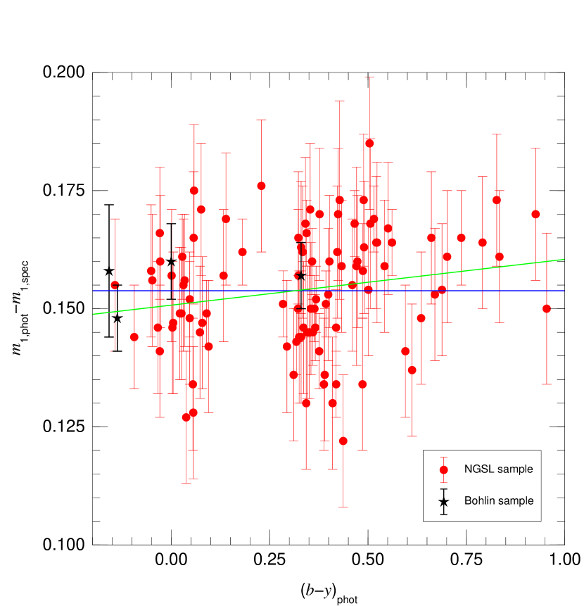
Figure 4: Comparison between photometric and spectrophotometric $m_{1}$ indices as a function of photometric $b-y$ for the NGSL + Bohlin samples. The error bars represent the photometric uncertainties and the horizontal blue line marks the proposed ZP${}_{m_{1}}$. The green line shows the result of a weighted linear fit to the data.

The zero point was calculated using inverse variance weighting to obtain $\mbox{ZP${}_{m_{1}}$}=0.154\pm 0.001$ mag. The difference between the zero point and the linear fits yields a 1-sigma systematic uncertainty of 0.003 mag and the uncertainty in the white dwarf calibration contributes with less than 0.001 magnitudes, as expected from the weak dependence of $m_{1}$ on temperature. The final result is then $\mbox{ZP${}_{m_{1}}$}=0.154\pm 0.001$ (random) $\pm 0.003$ (systematic) magnitudes.

4.4 $c_{1}$

I performed for $c_{1}$ an analysis similar to the one for $m_{1}$ using again the Matsushima (1969) sensitivity curves. The $(b-y)_{\rm phot}$ vs. $c_{1,{\rm phot}}-c_{1,{\rm spec}}$ plot in Fig. 5 clearly shows that a color term is present, with the bluer stars above the mean and the redder ones below it. The measured slope is $-0.045\pm 0.006$, which is 7.5 sigmas away from zero and the variation over the full range is $\pm 0.027$ magnitudes. Given the results I found for $b-y$ and $m_{1}$, I consider that variation too large to be tolerated as a systematic uncertainty. The likely culprit is one of the sensitivity curves and, given that I have previously determined that the Matsushima (1969) $b$ filter curve is correct and that the corresponding $v$ curve introduces only small errors in the synthetic magnitudes, I conclude that it is the $u$ curve definition the one that needs to be recalculated.

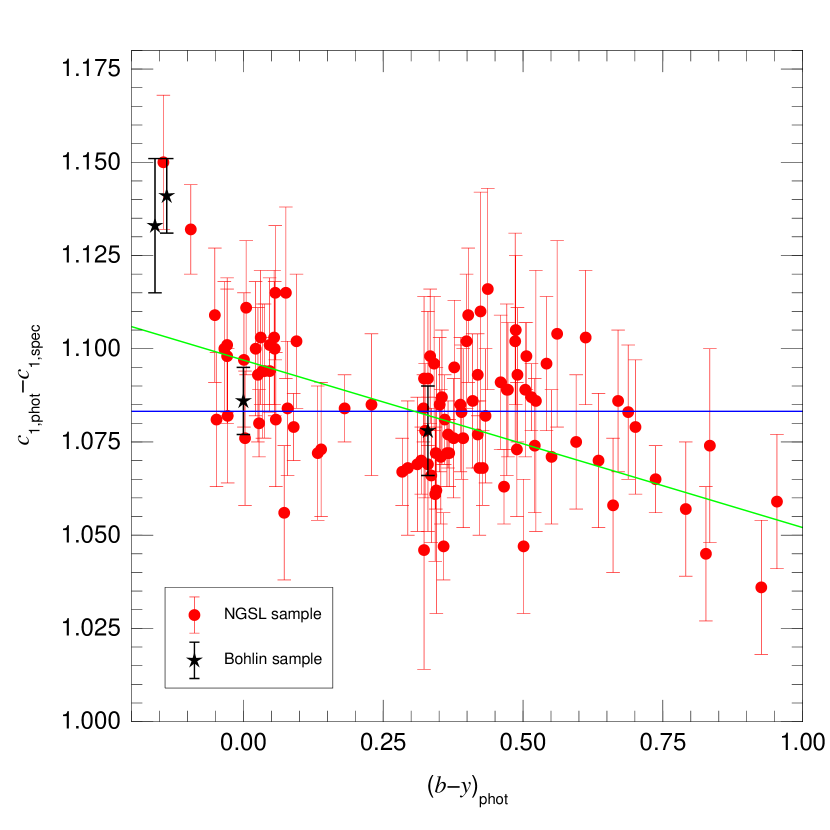
Figure 5: Comparison between photometric and spectrophotometric $c_{1}$ indices as a function of photometric $b-y$ for the NGSL + Bohlin samples using the Matsushima (1969) sensitivity curves. The error bars represent the photometric uncertainties and the horizontal blue line marks the weighted mean for the vertical coordinate. The green line shows the result of a weighted linear fit to the data.

A new Strömgren $u$ sensitivity curve was derived by $\chi^{2}$ minimization of $c_{1,{\rm phot}}-c_{1,{\rm spec}}$. I used a custom-made IDL code that includes the curve-fitting package written by Craig Markwardt, which allows for the fitting of an arbitrary function using $\chi^{2}$-minimization with restrictions on the parameters. I built the function in the following manner: (a) I selected 10 pivot wavelengths at 75 Å intervals between 3 150 Å and 3 825 Å. (b) The sensitivity at both extremes was fixed to be zero, given that we expect the result to be only slightly different from the Matsushima (1969) curve. (c) I placed additional constraints on the parameters to allow for a single-peaked function for the same reason. (d) This left nine free parameters to be fit, the sensitivity at the eight intermediate pivot wavelengths and ZP${}_{c_{1}}$. The initial guesses for the parameters were derived from the Matsushima (1969) $u$ curve. (e) The sensitivity curve between the pivot wavelengths was calculated using linear interpolation followed by smoothing with a box filter.

An initial run of the code produced a first estimate for both the sensitivity curve and ZP${}_{m_{1}}$, but the reduced $\chi^{2}$ was too large due to the underestimation of $\varepsilon_{c_{1}}$. The code was run several times, changing $\varepsilon_{c_{1}}$ until a value of 1.0 was reached for the reduced $\chi^{2}$. The sensitivity curve itself was found to change little between iterations. $\varepsilon_{c_{1}}$ was determined to be 0.009 mag and ZP${}_{c_{1}}$ (which here is one of the free parameters in the sensitivity-curve fitting procedure) to be $1.092\pm 0.002$ magnitudes. The old and new sensitivity curves for Strömgren $u$ are shown in Fig. 6, along with the sensitivity curves for Strömgren $v$ and $b$ and three selected spectra. The two curves for $u$ are found to be quite similar, with the only exception of the short-wavelength edge, which is redder by $\approx 35$ Å for the new result.

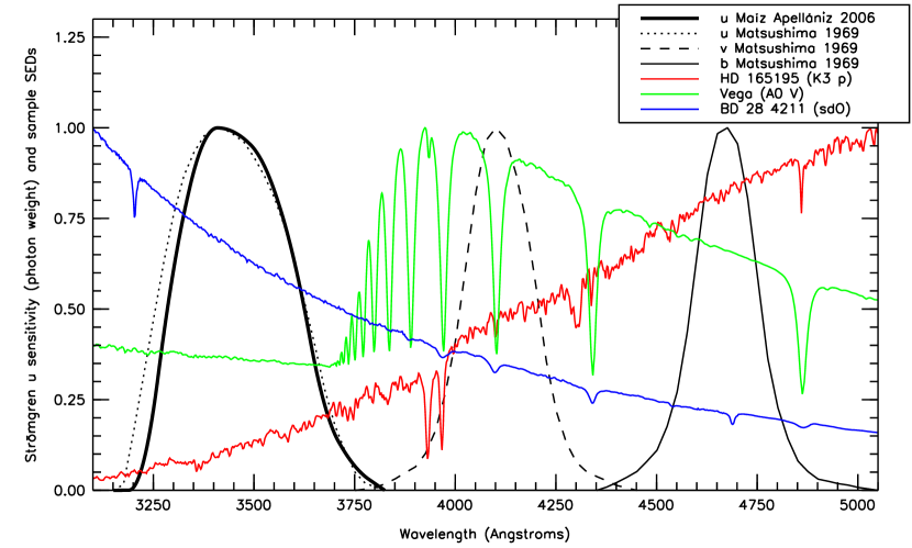
Figure 6: Matsushima (1969) photon-counting normalized sensitivity curves for the Strömgren $u$, $v$, and $b$ filters and the new curve for $u$ derived in this article. Three normalized SEDs from the two samples used to calibrate the Strömgren photometry are also shown as $f_{\lambda}$.

The new version of the $(b-y)_{\rm phot}$ vs. $c_{1,{\rm phot}}-c_{1,{\rm spec}}$ plot is shown in Fig. 7. As expected, the new curve does a much better job of fitting the data. The color term is now absent, as a weighted linear fit yields a slope of $-0.004\pm 0.006$, less than 1 sigma away from zero. Again, as for $b-y$ and $m_{1}$, no significant differences are perceived between the NGSL and Bohlin samples. The only outstanding issue is that the four bluest stars (two from the NGSL and two from the Bohlin samples) are still 1-3 sigmas above the zero point. In those cases the new sensitivity curve is a clear improvement (previously the same stars were 3-7 sigmas above the zero point) but the existence of such a residual systematic effect is likely a manifestation of the inherent difficulty of doing ground-based photometry to the left of the Balmer jump.

I can conclude that the new sensitivity curve does a better job of fitting the data than the old one (albeit not a perfect one). As for the error budget for the zero point, the slope of the fit contributes 0.001 mag to the systematic uncertainty and the uncertainty in the temperature scale (again, calculated from the different colors of high-gravity Kurucz models) adds 0.004 mag. Hence, I obtain $\mbox{ZP${}_{c_{1}}$}=1.092\pm 0.002$ (random) $\pm 0.004$ (systematic) magnitudes.

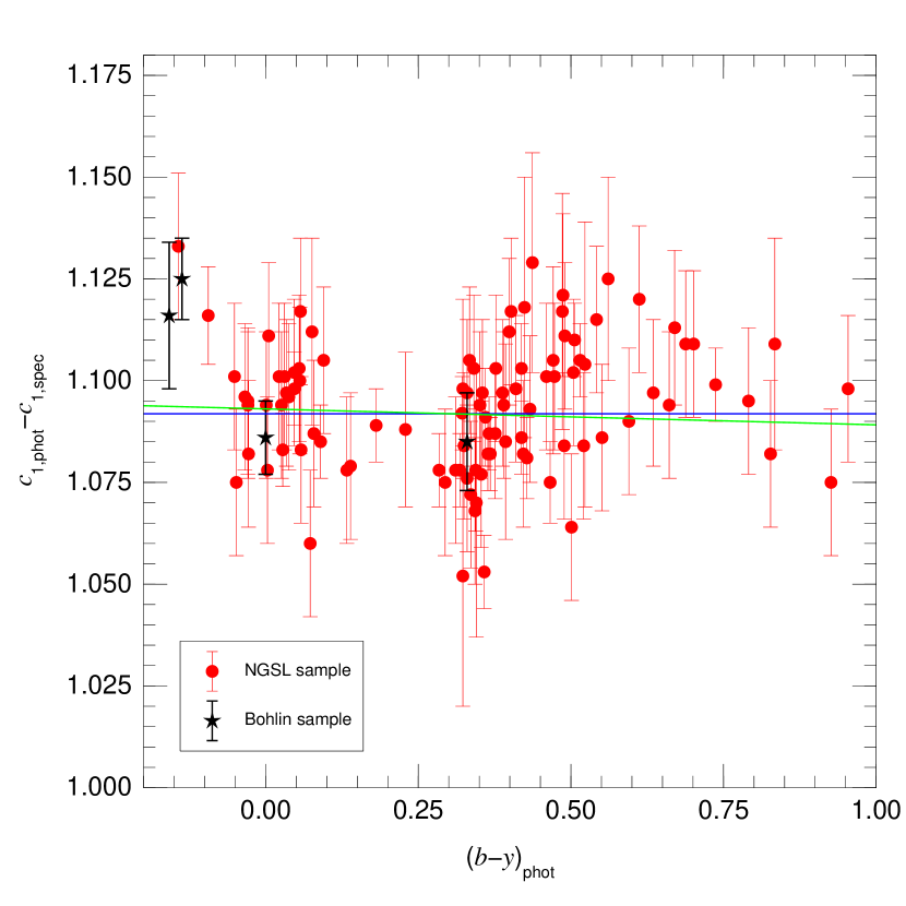
Figure 7: Comparison between photometric and spectrophotometric $c_{1}$ indices as a function of photometric $b-y$ for the NGSL + Bohlin samples using the sensitivity curves proposed in this article. The error bars represent the photometric uncertainties and the horizontal blue line marks the proposed ZP${}_{c_{1}}$. The green line shows the result of a weighted linear fit to the data.

5 Johnson $UBV$

5.1 Description and sample selection

The Johnson $UBV$ standard system (Johnson & Morgan, 1953) is the most commonly used broad-band optical photometry system. It covers a range of wavelengths similar to the Strömgren system but with only three filters. The quantities that are presented in most references are the $V$ magnitude and the two $B-V$ and $U-B$ colors. Both colors are a function mostly of temperature and extinction but metallicity and gravity effects are also present, especially at the lower stellar temperature end. $B-V$ is a rather monotonic function of temperature but for $T_{\rm eff}>20\,000$ K is almost degenerate. $U-B$ is more appropriate to measure temperatures for earlier spectral types, but the effect of the Balmer jump makes its dependence with temperature non-monotonic, especially for high-gravity stars.

A number of sensitivity curves for the $UBV$ system have been published over the years and a review can be found in Bessell (1990). That author found a relatively good agreement between different sources for the definitions of $B$ and $V$ but important differences in the definition of $U$. This can be seen by comparing the sensitivity functions proposed by Bessell (1990) with those of Buser & Kurucz (1978). The latter authors used the definitions for $B$ and $V$ by Ažusienis & Straižys (1969) and derived a new sensitivity function for $U$. As shown in Fig. 8, both sensitivity curves have similar red edges but the blue edge extends to considerably shorter wavelengths for the Bessell (1990) one.

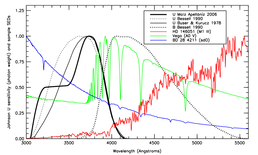
Figure 8: Bessell (1990) $U$ (UX) and $B$ (B) and Buser & Kurucz (1978) $U$ (U₃) photon-counting normalized sensitivity curves and the new curve for $U$ derived in this article. Three normalized SEDs from the two samples used to calibrate the Johnson photometry are also shown as $f_{\lambda}$.

Another important feature of both the Buser & Kurucz (1978) and Bessell (1990) studies is that two definitions for the $B$ sensitivity function are given depending on whether they are intended for computing $U-B$ or $B-V$. Hence, each of those papers gives four different sensitivity functions: Buser & Kurucz (1978) names them U₃, B₂, B₃, and V, with $\mbox{$U-B$}={\rm U}_{3}-{\rm B}_{2}$ and $\mbox{$B-V$}={\rm B}_{3}-{\rm V}$, while Bessell (1990) names them UX, BX, B, and V, with $\mbox{$U-B$}={\rm UX}-{\rm BX}$ and $\mbox{$B-V$}={\rm B}-{\rm V}$. This practice can be traced back to Ažusienis & Straižys (1969) as an attempt to correct for atmospheric extinction but it is quite obvious that it is unphysical: $B$ is $B$, independently of whether it is used to calculate $U-B$ or $B-V$.

In this section I test the sensitivity curves for the Johnson $UBV$ system. In order to build the photometric sample I used the GCPD and followed a selection procedure similar to the one in the previous section for the Strömgren system. The only relevant differences are:

1. I compiled one magnitude ($V$) and two colors ($B-V$ and $U-B$). For the four white dwarfs in Bohlin (2000) I used the values of $V$ in that reference and for Vega I used the value in Bohlin & Gilliland (2004b). The rest of the $V$ magnitudes and all of the colors are from the GCPD.

2. As opposed to Strömgren, the samples for $V$, $B-V$ and $U-B$ were built independently. However, the rules regarding the requirement of three data points for each star and the existence of 0.035 mag cutoffs in the random uncertainties were maintained.

3. The initial values for $\varepsilon_{V}$, $\varepsilon_{B-V}$, and $\varepsilon_{U-B}$ were set to zero.

After the selection process, 108, 111, and 101 stars were present in the $V$, $B-V$  and $U-B$ joint NGSL + Bohlin samples, respectively. 96 stars were present in the three samples and the 101 stars in the $U-B$ sample were also included in the $B-V$ sample. The numbers for $V$, $B$, and $B-V$ including only NGSL stars are 98, 104, and 96, respectively. The same numbers including only Bohlin stars are 10, 7, and 5, respectively.

5.2 $B-V$

The results for $B-V$ can be seen in Fig. 9. The plot uses the $B$ and $V$ sensitivity curves of Bessell (1990); I tried using the Buser & Kurucz (1978) and found that the results were very similar. $\varepsilon_{B-V}$ was iteratively determined to be 0.012 mag. The data does not show any significant trend with color, with a slope of the weighted linear fit of $-0.003\pm 0.003$, just 1 sigma away from zero. Also, no significant difference is observed between the NGSL and Bohlin samples. Therefore, I conclude that the Bessell (1990) sensitivity curves for $B$ and $V$ provide an accurate description for those filters.

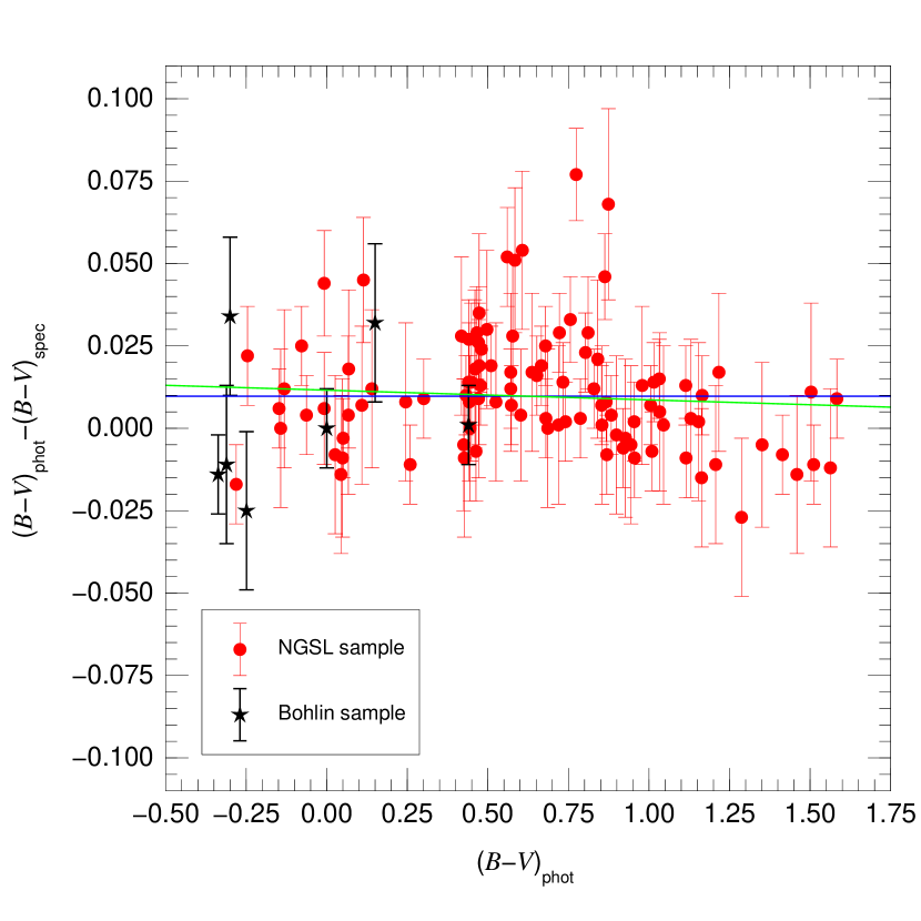
Figure 9: Comparison between photometric and spectrophotometric $B-V$ colors as a function of photometric $B-V$ for the NGSL and Bohlin $B-V$ samples. The error bars represent the photometric uncertainties and the horizontal blue line marks the proposed ZP_B-V. The green line shows the result of a weighted linear fit to the data.

The zero point was calculated using inverse variance weighting to obtain $\mbox{ZP${}_{B-V}$}=0.010\pm 0.001$ mag. For the systematic uncertainties I obtain 0.002 mag from the slope of the weighted linear fit and 0.003 mag from the temperature uncertainty in the white dwarf calibration. Therefore, I finally obtain $\mbox{ZP${}_{B-V}$}=0.010\pm 0.001$ (random) $\pm 0.004$ (systematic) magnitudes. It is interesting to point out that the photometric value for Vega itself compiled from the GCPD is $\mbox{$B-V$}=0.000\pm 0.012$ (with the uncertainty coming from $\varepsilon_{B-V}$), which is less than 1 sigma away from ZP_B-V. This is an additional confirmation of the consistency of the results.

5.3 $U-B$

I performed for $U-B$ an analysis similar to the one for $B-V$. Following the Strömgren $m_{1}$ and $c_{1}$ cases, I chose the equivalent of $b-y$ (i.e. $B-V$) as the comparison parameter since it provides a quasi-monotonic function of the spectral slope in the optical range. Given the differences between the Buser & Kurucz (1978) and Bessell (1990) $U$ sensitivity curves, the two cases were analyzed independently and the corresponding plots are shown in Fig. 10.

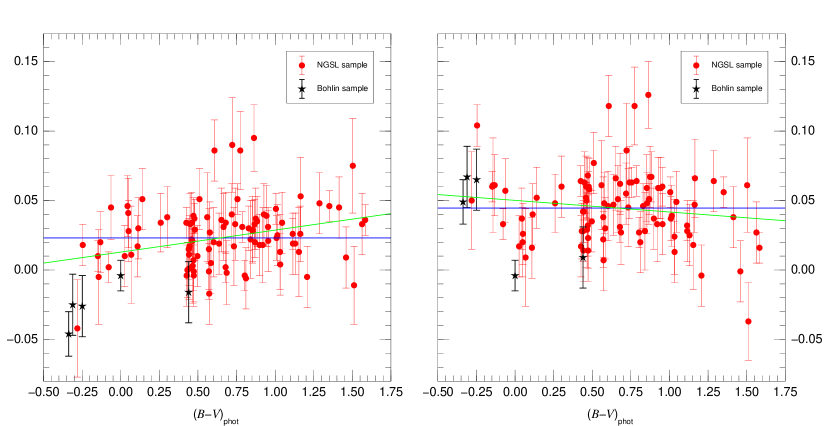
Figure 10: Comparison between photometric and spectrophotometric $U-B$ colors as a function of photometric $B-V$ for the NGSL and Bohlin $U-B$ samples. The left panel uses the sensitivity curve definitions of Buser & Kurucz (1978) and the right panel those of Bessell (1990). The error bars represent the photometric uncertainties and the horizontal blue line marks the weighted mean for the vertical coordinate in each panel. The green line shows the result of a weighted linear fit to the data in each panel.

The Buser & Kurucz (1978) plot (left panel of Fig. 10) shows a clear color term, with the bluer stars below the mean and the redder ones above it. The measured slope is $0.016\pm 0.004$, which is indeed 4 sigmas away from zero, leading to a variation over the full range of $\pm 0.016$ magnitudes, which is too much to be treated simply as a systematic error. Therefore, I conclude that the Buser & Kurucz (1978) sensitivity curves do not provide an adequate representation of the literature $U-B$ data.

The Bessell (1990) plot (right panel of Fig. 10) also shows a color term, though weaker and of the opposite sign as the Buser & Kurucz (1978), with the bluer stars above the mean and the redder ones below it. The measured slope is $-0.008\pm 0.004$, which is 2 sigmas away from zero and yields a variation over the full range of $\pm 0.008$ magnitudes. Such a variation is not very large but two additional issues exist. First, as previously mentioned, the calculation of the $U-B$ color using the Bessell (1990) definitions implies the unphysical use of a different sensitivity curve for $B$ than the one used for the same filter in the computation of the $B-V$ color. Second, the existence of a significant slope in the weighted linear fit to the data in the right panel of Fig. 10 is a manifestation of a more complex effect. As we go from left to right in the plot, we see first that the OB stars tend to be above the mean, then the A stars tend to be below it, the F and G again above it, and finally the K and M stars below it. This indicates that the considered $U$ sensitivity curve is not correctly assigning weights to the flux to the right and left of the Balmer jump. A consequence is that the derived ZP_U-B, 0.045, is very different from the photometric $U-B$ color for Vega, the reference star (A0 V), which is $-0.004$ magnitudes. Those arguments lead me to conclude that the Bessell (1990) sensitivity curves do not represent the literature $U-B$ data correctly, either.

The inadequacy of the existing $U$ sensitivity curves, which I previously discussed in Maíz Apellániz (2005b), led me to derive a new one using the same procedure I followed for Strömgren $u$. In this case I applied $\chi^{2}$ minimization to the $(\mbox{$U-B$})_{\rm phot}-(\mbox{$U-B$})_{\rm spec}$ data and used 12 pivot wavelengths at 100 Å intervals, setting the two extremes (where the sensitivity goes to zero) at 3 050 Å and 4 150 Å, respectively. Also, I eliminated the unphysical definition of an alternative $B$ filter and used the same one as for the $B-V$ zero point calculation. As it was the case for Strömgren $u$, several iterations with different values of $\varepsilon_{U-B}$ were required until a reduced $\chi^{2}$ of 1.0 was reached for $\varepsilon_{U-B}=0.011$.

The new $U$ sensitivity curve is shown in Fig. 8. As it happened for the Strömgren $u$ case, the red side of the curve is quite similar to the previous curves but the blue side is quite different. The function shows a steep rise around 3 100 Å followed by a plateau and a new rise around 3 600 Å. When the relative weights of the regions to the left and right of the Balmer jump are calculated, I find that the weight of the region to the left is smaller than for Bessell (1990) but larger than for Buser & Kurucz (1978). This is an expected effect, given the opposite slope of the weighted linear fits of the two plots in Fig. 10: a sensitivity curve with near-zero slope should lie at an intermediate point between the two previous ones. It should be pointed out that during the fitting procedure I found out that the exact shape of the sensitivity curve to the left of 3 600 Å is poorly constrained by the data, since alternative solutions (e.g. one with a small secondary peak maximum 3 300 Å) had similar values of $\chi^{2}$. This is also an expected result, since the 3 100-3 500 Å region contains little information in the form of strong absorption lines or edges. However, all of those alternative solutions had nearly constant integrated weights for the regions to the left and the right of the Balmer jump and, therefore, produced little variation in the derived synthetic $U-B$. Furthermore, it is important to remember that, as I mentioned in the introduction, it is likely that no single sensitivity curve can fit all the existing data: the purpose of this calculation is to find the sensitivity curve that minimizes systematic errors.

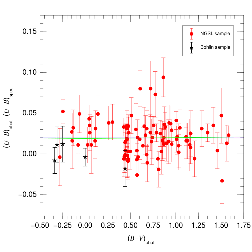
Figure 11: Comparison between photometric and spectrophotometric $U-B$ colors as a function of photometric $B-V$ for the NGSL and Bohlin $U-B$ samples using the sensitivity curve definitions proposed in this article. The error bars represent the photometric uncertainties and the horizontal blue line marks the proposed ZP_U-B. The green line shows the result of a weighted linear fit to the data.

The new version of the $(\mbox{$B-V$})_{\rm phot}$ vs. $(\mbox{$U-B$})_{\rm phot}-(\mbox{$U-B$})_{\rm spec}$ is shown in Fig. 11. As expected, the color term is absent, with the slope of the weighted linear fit being $0.001\pm 0.004$. The value for ZP_U-B, obtained from the sensitivity-curve $\chi^{2}$ minimization procedure, is $0.020\pm 0.006$ magnitudes. The systematic uncertainty from the fitted slope is very small ($<0.001$ mag) and the one from the uncertainty in the white dwarf temperature scale is 0.007 magnitudes. ZP_U-B is now considerably closer to the measured photometric $U-B$ color of Vega but, for $\varepsilon_{U-B}=0.011$, is still 2 sigmas away. Also, it should be noted that the five stars in the Bohlin sample appear to be shifted downward by $\approx 0.02$ magnitudes with respect to the mean locus of the NGSL sample in Fig. 11. It is unlikely that the source of the relative displacement is due to a problem with an incorrect relative calibration of spectrophotometry of the NGSL sample with respect to the Bohlin sample (as it was the case for Tycho-2 in Maíz Apellániz 2005a) since such a displacement should also show up in Fig. 7, given the similar wavelengths sampled by $U$ and $u$. The effect could simply be a case of small number statistics (the probability that all of five points in a Gaussian distribution lie at the same side of the mean is 1/16) but, to be conservative, I suggest that the systematic uncertainty be doubled to take into account the possibility that the difference between the results for the NGSL and the Bohlin samples is real. Therefore, the proposed value for ZP_U-B is $0.020\pm 0.006$ (random) $\pm 0.014$ (systematic) magnitudes.

5.4 $V$

Up until now I have dealt with the calibration of colors and indices but not of magnitudes themselves. In the first case the accuracy of the calibration depends ultimately on the parameters (fundamentally temperature) of the spectrophotometric standards and on the stability and knowledge of the observational photometric conditions. The same is true for magnitudes but there one also runs into the spectrophotometric absolute flux calibration. That issue has been tackled by Bohlin (2000) and Bohlin & Gilliland (2004b), who combined the 5 556 Å absolute flux of Vega of Mégessier (1995), Landolt $V$ photometry for the three white dwarfs used as primary calibrators, and STIS spectrophotometry to derive a $V$ value for Vega of $0.026\pm 0.008$ magnitudes.

Trying to use the Bohlin sample to derive a value for ZP_V using the same procedure as for e.g. $B-V$ would be falling into a logical inconsistency: the $V$ photometry of the white dwarf calibrators and their HST spectrophotometry are not independent, since the absolute calibration of the second has been derived using the first as input. Therefore, the fact that the $V_{\rm phot}-V_{\rm spec}$ values for the Bohlin sample in Fig. 12 show no trend with $V_{\rm phot}$ or $(\mbox{$B-V$})_{\rm phot}$ is simply a verification that the spectrophotometric calibration is self-consistent. A similar argument takes place with the value of ZP_V. In the Bohlin sample there are five stars where the $V$ magnitudes are taken from the two references above plus another four stars with accurate photometry in the GCPD (however, only six stars have also accurate $B-V$ photometric colors in our data). The weighted mean of $V_{\rm phot}-V_{\rm spec}$ yields 0.024, which is very close to the $V$ magnitude of Vega. And what about using the NGSL sample to calculate ZP_V? Unfortunately, there one runs into the same problem as for ZP${}_{V_{\rm T}}$ or ZP${}_{B_{\rm T}}$ in Paper I: the NGSL data cannot be used to directly calculate the zero point of a magnitude because they were obtained with the 52X0.2 slit, so significant light losses due to miscenterings are to be expected. Indeed, that effect is clearly seen in Fig. 12 in a similar manner to what happens in Fig. 4 in Paper I. Therefore, the most appropriate choice for ZP_V is the $V$ magnitude for Vega, $0.026\pm 0.008$, derived by Bohlin & Gilliland (2004b).

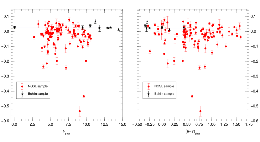
Figure 12: Comparison between photometric and spectrophotometric $V$ magnitudes as a function of the photometric values for $V$ (left) and $B-V$ (right) for the NGSL + Bohlin samples. The error bars represent the photometric uncertainties and the horizontal line marks the proposed ZP_V. The asymmetric scatter of values below the line is due to light loss at the slit due to poor centering.

5.5 A new look at the absolute calibration of Tycho-2 photometry

In Paper I the $V_{\rm T}$ filter was calibrated through the $B_{\rm T}$ photometry for the Bohlin sample and the ZP${}_{B_{\rm T}-V_{\rm T}}$ derived from the combination of the NGSL and Bohlin samples. Since the last term is now known to have been in error, a new value for ZP${}_{V_{\rm T}}$ needs to be calculated. If I use the four stars in the Bohlin sample with accurate $V_{\rm T}$ photometry and calculate the mean of $\mbox{$V_{\rm T}$}_{\rm phot}-\mbox{$V_{\rm T}$}_{\rm spec}$ using inverse variance weights I obtain $0.039\pm 0.008$ magnitudes (see right panel of Fig. 4 in Paper I). Note that the uncertainty originates in the Tycho-2 photometry, not in the the Vega $V$ magnitude. It is interesting to notice that if the absolute HST calibration were to be off by a multiplicative constant (let’s say 1%), it would not affect that measurement of ZP${}_{V_{\rm T}}$ because the zero point is measured by comparing two spectrophotometric fluxes on the same scale (e.g. the multiplicative constant would affect both the numerator and the denominator in Eq. A1). A different issue, of course, would be the absolute zero point as defined by Eq. B2.

The availability of the Johnson $V$ photometry allows me to perform an independent measurement of ZP${}_{V_{\rm T}}$. $V_{\rm T}$ and $V$ measure the flux in a similar wavelength range (Bessell, 2000) but are also different enough that $V_{\rm T}-V$ varies by $\approx 0.26$ magnitudes as we move along the unreddened main sequence. In any case, since the $V_{\rm T}$ and $V$ photometric measurements are independent, I can compile photometric $V_{\rm T}-V$ values and compare them with the computed spectrophotometric ones to derive ZP${}_{V_{\rm T}-V}$. The results are shown in Fig. 13. There is a color term present but the slope is quite small, $0.008\pm 0.004$, and is only 2 sigmas away from zero so, as I have done for other colors, the effect can be simply included as a systematic uncertainty. Using inverse variance weights I obtain $\mbox{ZP${}_{V_{\rm T}-V}$}=0.000\pm 0.002$ magnitudes. For the systematic uncertainty there are 0.005 magnitudes due to the color term and 0.001 magnitudes due to the uncertainty in the white dwarf temperature scale, leading to a final value of $\mbox{ZP${}_{V_{\rm T}-V}$}=0.000\pm 0.002$ (random) $\pm 0.005$ (systematic) magnitudes. ZP${}_{V_{\rm T}}$ can now be obtained by adding the ZP_V value from the previous subsection. Merging random and systematic uncertainties for simplicity, I get $\mbox{ZP${}_{V_{\rm T}}$}=0.026\pm 0.010$.

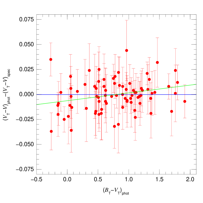
Figure 13: Comparison between photometric and spectrophotometric $V_{\rm T}-V$ magnitudes as a function of the photometric values $B_{\rm T}-V_{\rm T}$ (right) for the NGSL sample. The error bars represent the photometric uncertainties and the horizontal line marks the proposed ZP${}_{V_{\rm T}-V}$. The green line shows the result of a weighted linear fit to the data.

The measurements of ZP${}_{V_{\rm T}}$ in the two previous paragraph are independent and compatible, as they are just one sigma away ($[0.039-0.026]/\sqrt{0.008^{2}+0.010^{2}}=1.0$). Furthermore, since there are no systematic uncertainties in common in the two derivations, they can be combined using inverse variance weights to obtain a best value for ZP${}_{V_{\rm T}}$ of $0.034\pm 0.006$.

The value for ZP${}_{B_{\rm T}}$ derived in Paper I from the Bohlin sample is $0.078\pm 0.009$. If I combine this with the new value for ZP${}_{V_{\rm T}}$ (derived from the NGSL $V_{\rm T}-V$ colors and from Bohlin & Gilliland 2004b) I obtain an alternative measurement for ZP${}_{B_{\rm T}-V_{\rm T}}$ of $0.044\pm 0.011$ magnitudes, which is consistent with the result of $0.033\pm 0.001$ (random) $\pm 0.005$ (systematic) previously derived, thus providing an additional check on the validity of the zero points.

6 Summary and applications

I have analyzed the sensitivity curves for the Tycho-2, Strömgren, and Johnson photometric systems and have determined that for 7 of the 9 curves there are values in the literature consistent with the available photometry and HST spectrophotometry. The recommended photon-counting sensitivity curves are given in Tables 1, 2, and 3. The results for $B_{\rm T}$ and $V_{\rm T}$ are taken from Bessell (2000), for Strömgren $vby$ from Matsushima (1969), and for Johnson $BV$ from Bessell (1990) and have been converted in all cases into photon counting curves. The results for Strömgren $u$ and Johnson $U$ have been derived in this paper after finding that the published curves do not provide consistent results with both the photometry and the spectrophotometry. For those two cases, the differences between the literature and the new curves reside on the blue edge of a filter centered around 3 400-3 700 Å, which indicates that the likely culprit is an incorrect characterization of atmospheric extinction.

I show in Tables 4 and 5 the recommended zero points for the colors, indices, and magnitudes calculated in this article. All zero points use Vega as the reference spectrum. In Table 5 I also include the zero points for $y$ computed by Holberg & Bergeron (2006) and for the 2MASS system computed by Cohen et al. (2003).

Recently, Holberg & Bergeron (2006) have combined optical/IR photometry and SED models of very low extinction DA white dwarfs with the Bohlin (2000) HST flux calibration to derive results similar to the ones in this paper. Their color/index zero points for the Strömgren and Johnson systems are independent from the ones here because they are based on a largely different sample and because they use model SEDs instead of observed ones. Their values for ZP_b-y, ZP${}_{m_{1}}$, and ZP_B-V are 0.004, 0.154, and 0.007 magnitudes, respectively, all of which agree within 1 sigma with the ones in this paper. Since those authors do not attempt to fit Strömgren $u$ or Johnson $U$ sensitivity curves, it is not possible to compare their zero points for $c_{1}$ and $U-B$ directly with mine. However, the fact that their Strömgren data show the highest scatter for the $u$ band and that their Johnson filter with the largest dispersion is $U$ points in the same direction as my conclusion that new sensitivity curves are required in those two cases. Therefore, the results in the two articles are consistent.

   

Figure 14: Comparison between the photometric and spectrophotometric Strömgren values for the individual data points in the GCPD. The left, center, and right panels show $b-y$  $m_{1}$, and $c_{1}$, respectively. Gaussians with zero mean and $\sigma$ of 0.013, 0.014, and 0.018 magnitudes, respectively, are plotted for comparison.

 

Figure 15: Comparison between the photometric and spectrophotometric Johnson values for the individual data points in the GCPD. The left and right panels show $B-V$ and $U-B$, respectively. Gaussians with zero mean and $\sigma$ of 0.020 and 0.028 magnitudes, respectively, are plotted for comparison.

The most direct application of this work is the use of the zero points in Tables 4 and 5 and of the two new sensitivity curves for synthetic photometry. The latest version of CHORIZOS (Maíz Apellániz, 2004) at the time of this publication (2.0) incorporates them. Another application is to provide uncertainties for the Strömgren and Johnson colors and indices in the GCPD. To do the latter, I start with the photometry originally compiled in sections 4 and 5. For each data point for each star in the NGSL sample I can now compute the difference between the photometric and spectrophotometric values for each color and index and obtain the corresponding distributions. The total number of data points for each of the five colors/indices turns out to be between 662 and 871, much larger than the numbers used to test the sensitivity curves because now all stars in the sample are used and no average is done for each star; in this way one can obtain an estimate for the typical uncertainty associated with a literature value. The distributions are shown in Figs. 14 and 15 and can be well approximated by a Gaussian plus tails. The tails are defined as being more than 3.5 sigmas away from the mean, with the standard deviation calculated iteratively. The value of 3.5 sigmas is chosen because $1/[1-{\rm errorf}(3.5/\sqrt{2})]=2\,149$, implying that a sample of roughly three times the ones we have here are required for at least one data point to be at larger distances from the mean. For each color/index I find that 2-6% of the data points are in the tails and I take those objects to be either misidentifications or cases with incorrect data reductions. Hence, they are not considered for the subsequent analysis.

The mean for the distributions of $(\mbox{$b-y$})_{\rm phot}-(\mbox{$b-y$})_{\rm spec}$, $\mbox{$m_{1}$}_{\rm phot}-\mbox{$m_{1}$}_{\rm spec}$, and $\mbox{$c_{1}$}_{\rm phot}-\mbox{$c_{1}$}_{\rm spec}$ are all within 0.001 magnitudes of the corresponding zero points. The dispersions, which can be taken to be the estimates for the uncertainty associated with a single data point in the GCPD, are 0.013, 0.014, and 0.018 magnitudes, respectively. These results provide an additional check to the validity of the sensitivity curves and zero points calculated in this article and show that the typical precision for a single value of a Strömgren color or index in the literature is $1-2$%. In Tables 6, 7, and 8 the dispersions are given as a function of $V$ magnitude and $N$, the number of measurements used for an individual data point (Hauck & Mermilliod, 1998). The variation with $V$ and $N$ is in the expected direction (brighter stars or those with more measurements have lower dispersions) but the effect is very small, so using a single value for the photometric uncertainty should not be a bad approximation.

The mean for the distributions of $(\mbox{$B-V$})_{\rm phot}-(\mbox{$B-V$})_{\rm spec}$ and $(\mbox{$U-B$})_{\rm phot}-(\mbox{$U-B$})_{\rm spec}$ are 0.0016 and 0.0022 magnitudes larger than the respective zero points, slightly larger than for the Strömgren cases but still within the values expected from the uncertainties derived for ZP_B-V and ZP_U-B. The associated dispersions are 0.020 and 0.028 magnitudes, also slightly larger than in the Strömgren cases. The results in Tables 9 and 10 show a weak dependency of the dispersions with $V$ and a negligible dependence with $N$, so a single value for the photometric uncertainty should also be appropriate for Johnson photometry. I conclude that the typical precision for $B-V$ and $U-B$ values in the literature is in the $2-3$% range, slightly larger than for Strömgren.

Appendix A Photon- and energy-counting detectors

When computing synthetic magnitudes from spectrophotometry, one has to be careful with an aspect that has generated some confusion in the past. For a photon-counting detector, such as a CCD, given the total-system dimensionless sensitivity function $P(\lambda)$, the SED of the object $f_{\lambda}(\lambda)$, the SED of the reference spectrum $f_{\lambda{\rm,ref}}(\lambda)$, and the zero point ZP_P for filter $P$, the corresponding magnitude is given by:

$$m_{P}=-2.5\log_{10}\left(\frac{\int P(\lambda)f_{\lambda}(\lambda)\lambda\,d\lambda}{\int P(\lambda)f_{\lambda{\rm,ref}}(\lambda)\lambda\,d\lambda}\right)+{\rm ZP}_{P}.$$ (A1)

The $\lambda$ inside the integrals in Eq. A1 is present because $f_{\lambda}(\lambda)$ is in units of energy per time per unit area per wavelength and one needs to multiply by $\lambda/(hc)$ in order to convert from energy to photons (the $hc$ disappears because it is a constant that appears on both integrals). For an energy-counting (or energy-integrating) detector, the $\lambda$ is not present and the corresponding magnitude is given by:

$$m_{P}^{\prime}=-2.5\log_{10}\left(\frac{\int P^{\prime}(\lambda)f_{\lambda}(\lambda)\,d\lambda}{\int P^{\prime}(\lambda)f_{\lambda{\rm,ref}}(\lambda)\,d\lambda}\right)+{\rm ZP}^{\prime}_{P^{\prime}},$$ (A2)

where $P^{\prime}(\lambda)$ and ZP${}^{\prime}_{P^{\prime}}$ are the sensitivity function and the zero point, respectively.

It is easy to verify that one can use either Eq. A1 or Eq. A2 independently of the physical type of detector involved if the sensitivity function is changed accordingly. For example, suppose I want to use Eq. A1 with an energy-counting detector. If one multiplies and divides by $\lambda$ the quantities inside the two integrals in Eq. A2 and defines $P(\lambda)=P^{\prime}(\lambda)/\lambda$ and ZP_P = ZP${}^{\prime}_{P^{\prime}}$ to be the photon-equivalent sensitivity function and zero point, respectively, then Eq. A1 is recovered (this is the reason why previous works, such as Bessell et al. 1998, can be correct even though they use energy-integrating sensitivities).

The problem that has arisen sometimes is that Eq. A1 has been used with an energy-counting sensitivity function without first dividing it by $\lambda$ to convert it to a photon-equivalent sensitivity function. The likely origin of the confusion has been the old practice of defining sensitivity functions for photomultipliers as energy-counting combined with the present extensive use of “black-box” synthetic photometry codes such as synphot designed for photon-counting detectors.

Appendix B Absolute and relative zero points

ZP_P, the zero point used in the previous section is a relative zero point, since a reference spectrum is used to define it. In a number of magnitude systems (typically, those defined with synthetic photometry in mind), such as VEGAMAG, STMAG, or ABMAG (STScI, 1998), ZP${}_{P}=0.0$ by definition and the calibration information is contained in the reference spectrum alone. For other magnitude systems derived from standard stars, ZP_P is not exactly zero and has to be measured (that is one of the main purposes of this paper), although it is possible that if the right reference spectrum is used (e.g. Vega) ZP_P can be indeed approximately zero. However, one can also avoid altogether the reference spectrum in the definition of a magnitude system by using (for a photon-counting detector):

$$m_{P}=-2.5\log_{10}\left(\int P(\lambda)f_{\lambda}(\lambda)\lambda\,d\lambda\right)+{\rm AZP}_{P},$$ (B1)

where AZP_P is the absolute zero point for filter $P$, which is related to ZP_P by:

$${\rm AZP}_{P}=2.5\log_{10}\left(\int P(\lambda)f_{\lambda{\rm,ref}}(\lambda)\lambda\,d\lambda\right)+{\rm ZP}_{P}.$$ (B2)

Note that the quantities inside the parenthesis in Eqs. B1 and B2 are not dimensionless (they have dimensions of energy per time per length), so the units used must be specified when values for AZP_P are given.

Table 1: Recommended photon-counting sensitivity curves for the Tycho $B_{\rm T}$$V_{\rm T}$ system

$B_{\rm T}$			$V_{\rm T}$
$\lambda$ (Å)	$P(\lambda)$		$\lambda$ (Å)	$P(\lambda)$
3500	0.000		4550	0.000
3550	0.014		4600	0.022
3600	0.058		4650	0.115
3650	0.123		4700	0.302
3700	0.206		4750	0.532
3750	0.305		4800	0.740
3800	0.416		4850	0.873
3850	0.530		4900	0.944
3900	0.636		4950	0.977
3950	0.724		5000	0.994
4000	0.787		5050	1.000
4050	0.830		5100	0.995
4100	0.861		5150	0.979
4150	0.889		5200	0.953
4200	0.920		5250	0.920
4250	0.953		5300	0.882
4300	0.982		5350	0.840
4350	1.000		5400	0.797
4400	0.976		5450	0.752
4450	0.861		5500	0.707
4500	0.685		5550	0.661
4550	0.489		5600	0.614
4600	0.317		5650	0.567
4650	0.202		5700	0.520
4700	0.136		5750	0.473
4750	0.101		5800	0.426
4800	0.080		5850	0.381
4850	0.059		5900	0.336
4900	0.036		5950	0.294
4950	0.016		6000	0.255
5000	0.003		6050	0.219
5050	0.000		6100	0.187
$\cdots$	$\cdots$		6150	0.160
$\cdots$	$\cdots$		6200	0.136
$\cdots$	$\cdots$		6250	0.114
$\cdots$	$\cdots$		6300	0.097
$\cdots$	$\cdots$		6350	0.082
$\cdots$	$\cdots$		6400	0.069
$\cdots$	$\cdots$		6450	0.058
$\cdots$	$\cdots$		6500	0.047
$\cdots$	$\cdots$		6550	0.038
$\cdots$	$\cdots$		6600	0.028

Table 2: Recommended photon-counting sensitivity curves for the Strömgren $uvby$ standard system

$u$			$v$			$b$			$y$
$\lambda$ (Å)	$P(\lambda)$		$\lambda$ (Å)	$P(\lambda)$		$\lambda$ (Å)	$P(\lambda)$		$\lambda$ (Å)	$P(\lambda)$
3150	0.000		3750	0.000		4350	0.000		5150	0.000
3175	0.000		3775	0.003		4375	0.009		5175	0.013
3200	0.007		3800	0.008		4400	0.021		5200	0.033
3225	0.076		3825	0.018		4425	0.035		5225	0.054
3250	0.220		3850	0.031		4450	0.051		5250	0.079
3275	0.424		3875	0.048		4475	0.079		5275	0.136
3300	0.607		3900	0.064		4500	0.109		5300	0.199
3325	0.758		3925	0.100		4525	0.173		5325	0.296
3350	0.879		3950	0.162		4550	0.267		5350	0.452
3375	0.961		3975	0.268		4575	0.428		5375	0.637
3400	0.999		4000	0.410		4600	0.644		5400	0.793
3425	1.000		4025	0.609		4625	0.861		5425	0.879
3450	0.990		4050	0.813		4650	0.979		5450	0.926
3475	0.972		4075	0.960		4675	1.000		5475	0.964
3500	0.945		4100	1.000		4700	0.959		5500	1.000
3525	0.898		4125	0.970		4725	0.815		5525	0.982
3550	0.830		4150	0.878		4750	0.597		5550	0.872
3575	0.742		4175	0.748		4775	0.375		5575	0.672
3600	0.634		4200	0.568		4800	0.236		5600	0.479
3625	0.503		4225	0.367		4825	0.147		5625	0.302
3650	0.357		4250	0.224		4850	0.084		5650	0.193
3675	0.239		4275	0.135		4875	0.053		5675	0.127
3700	0.157		4300	0.080		4900	0.032		5700	0.080
3725	0.107		4325	0.053		4925	0.025		5725	0.048
3750	0.068		4350	0.039		4950	0.019		5750	0.026
3775	0.039		4375	0.027		4975	0.015		5775	0.018
3800	0.019		4400	0.014		5000	0.008		5800	0.015
3825	0.000		4425	0.007		5025	0.004		5825	0.008
$\cdots$	$\cdots$		4450	0.000		5050	0.000		5850	0.000

Table 3: Recommended photon-counting sensitivity curves for the Johnson $UBV$ standard system

$U$			$B$			$V$
$\lambda$ (Å)	$P(\lambda)$		$\lambda$ (Å)	$P(\lambda)$		$\lambda$ (Å)	$P(\lambda)$
3050	0.000		3600	0.000		4700	0.000
3100	0.237		3650	0.011		4750	0.004
3150	0.403		3700	0.033		4800	0.032
3200	0.489		3750	0.058		4850	0.084
3250	0.504		3800	0.144		4900	0.172
3300	0.508		3850	0.348		4950	0.310
3350	0.511		3900	0.601		5000	0.478
3400	0.513		3950	0.817		5050	0.650
3450	0.516		4000	0.958		5100	0.802
3500	0.528		4050	1.000		5150	0.913
3550	0.603		4100	0.995		5200	0.978
3600	0.741		4150	0.995		5250	1.000
3650	0.889		4200	0.994		5300	0.994
3700	0.985		4250	0.976		5350	0.977
3750	1.000		4300	0.950		5400	0.950
3800	0.965		4350	0.921		5450	0.911
3850	0.841		4400	0.888		5500	0.862
3900	0.648		4450	0.845		5550	0.806
3950	0.424		4500	0.792		5600	0.747
4000	0.231		4550	0.733		5650	0.690
4050	0.109		4600	0.673		5700	0.634
4100	0.035		4650	0.619		5750	0.579
4150	0.000		4700	0.569		5800	0.523
$\cdots$	$\cdots$		4750	0.519		5850	0.467
$\cdots$	$\cdots$		4800	0.467		5900	0.413
$\cdots$	$\cdots$		4850	0.414		5950	0.363
$\cdots$	$\cdots$		4900	0.362		6000	0.317
$\cdots$	$\cdots$		4950	0.315		6050	0.274
$\cdots$	$\cdots$		5000	0.272		6100	0.234
$\cdots$	$\cdots$		5050	0.232		6150	0.200
$\cdots$	$\cdots$		5100	0.193		6200	0.168
$\cdots$	$\cdots$		5150	0.155		6250	0.140
$\cdots$	$\cdots$		5200	0.121		6300	0.114
$\cdots$	$\cdots$		5250	0.096		6350	0.089
$\cdots$	$\cdots$		5300	0.075		6400	0.067
$\cdots$	$\cdots$		5350	0.054		6450	0.050
$\cdots$	$\cdots$		5400	0.034		6500	0.037
$\cdots$	$\cdots$		5450	0.018		6550	0.027
$\cdots$	$\cdots$		5500	0.007		6600	0.020
$\cdots$	$\cdots$		5550	0.001		6650	0.016
$\cdots$	$\cdots$		5600	0.000		6700	0.013
$\cdots$	$\cdots$		$\cdots$	$\cdots$		6750	0.012
$\cdots$	$\cdots$		$\cdots$	$\cdots$		6800	0.010
$\cdots$	$\cdots$		$\cdots$	$\cdots$		6850	0.009
$\cdots$	$\cdots$		$\cdots$	$\cdots$		6900	0.007
$\cdots$	$\cdots$		$\cdots$	$\cdots$		6950	0.004
$\cdots$	$\cdots$		$\cdots$	$\cdots$		7000	0.000

Table 4: Color/index zero points and associated uncertainties/errors.

	Tycho-2		Strömgren				Johnson
	$B_{\rm T}-V_{\rm T}$		$b-y$	$m_{1}$	$c_{1}$		$B-V$	$U-B$
zero point	0.033		0.007	0.154	1.092		0.010	0.020
random	0.001		0.001	0.001	0.002		0.001	0.006
systematic	0.005		0.003	0.003	0.004		0.004	0.014

Table 5: Magnitude zero points and associated uncertainties. The values for $y$ are from Holberg & Bergeron (2006) and those for the 2MASS filters from Cohen et al. (2003).

	Tycho-2		Strömgren		Johnson		2MASS
	$V_{\rm T}$		$y$		$V$		$J$	$H$	$K_{\rm s}$
zero point	0.034		0.014		0.026		$-$0.001	0.019	$-$0.017
uncertainty	0.006		0.010		0.008		0.005	0.007	0.005

Table 6: Dispersions for $(\mbox{$b-y$})_{\rm phot}-(\mbox{$b-y$})_{\rm spec}$ as a function of $V$ and $N$ for all the data points (excluding 3.5 sigma outliers).

	$N$
	$\leq 3$	$\geq 4$	All
$V\leq 6.0$	0.012	0.011	0.012
$V>6.0$	0.014	0.013	0.014
All	0.014	0.013	0.013

Table 7: Dispersions for $\mbox{$m_{1}$}_{,\rm phot}-\mbox{$m_{1}$}_{,\rm spec}$ as a function of $V$ and $N$ for all the data points (excluding 3.5 sigma outliers).

	$N$
	$\leq 3$	$\geq 4$	All
$V\leq 6.0$	0.013	0.012	0.012
$V>6.0$	0.015	0.013	0.014
All	0.014	0.013	0.014

Table 8: Dispersions for $\mbox{$c_{1}$}_{,\rm phot}-\mbox{$c_{1}$}_{,\rm spec}$ as a function of $V$ and $N$ for all the data points (excluding 3.5 sigma outliers).

	$N$
	$\leq 3$	$\geq 4$	All
$V\leq 6.0$	0.018	0.015	0.017
$V>6.0$	0.019	0.018	0.018
All	0.018	0.017	0.018

Table 9: Dispersions for $(\mbox{$B-V$})_{\rm phot}-(\mbox{$B-V$})_{\rm spec}$ as a function of $V$ and $N$ for all the data points (excluding 3.5 sigma outliers).

	$N$
	$\leq 3$	$\geq 4$	All
$V\leq 6.0$	0.017	0.018	0.018
$V>6.0$	0.020	0.024	0.022
All	0.019	0.020	0.020

Table 10: Dispersions for $(\mbox{$U-B$})_{,\rm phot}-(\mbox{$U-B$})_{,\rm spec}$ as a function of $V$ and $N$ for all the data points (excluding 3.5 sigma outliers).

	$N$
	$\leq 3$	$\geq 4$	All
$V\leq 6.0$	0.026	0.029	0.028
$V>6.0$	0.030	0.027	0.029
All	0.028	0.028	0.028

References

- Ažusienis & Straižys (1969) Ažusienis, A., & Straižys, V. 1969, Soviet Astronomy, 13, 316
- Bessell (1990) Bessell, M. S. 1990, PASP, 102, 1181
- Bessell (2000) —. 2000, PASP, 112, 961
- Bessell et al. (1998) Bessell, M. S., Castelli, F., & Plez, B. 1998, A&A, 333, 231
- Bianchi et al. (1999) Bianchi, L., et al. 1999, Mem. Soc. Astron. Ital., 70, 365
- Bohlin (2000) Bohlin, R. C. 2000, AJ, 120, 437
- Bohlin et al. (2001) Bohlin, R. C., Dickinson, M. E., & Calzetti, D. 2001, AJ, 122, 2118
- Bohlin & Gilliland (2004a) Bohlin, R. C., & Gilliland, R. L. 2004a, AJ, 128, 3053
- Bohlin & Gilliland (2004b) —. 2004b, AJ, 127, 3508
- Buser & Kurucz (1978) Buser, R., & Kurucz, R. L. 1978, A&A, 70, 555
- Cohen et al. (2003) Cohen, M., Wheaton, W. A., & Megeath, S. T. 2003, AJ, 126, 1090
- ESA (1997) ESA. 1997, The Hipparcos and Tycho Catalogues (ESA SP-1200)
- Gregg et al. (2004) Gregg, M. D., Silva, D., Rayner, J., Valdes, F., Worthey, G., Pickles, A., Rose, J. A., Vacca, W., & Carney, B. 2004, American Astronomical Society Meeting Abstracts, 205
- Hauck & Mermilliod (1998) Hauck, B., & Mermilliod, M. 1998, A&AS, 129, 431
- Holberg & Bergeron (2006) Holberg, J. B., & Bergeron, P. 2006, AJ (submitted)
- Johnson & Morgan (1953) Johnson, H. L., & Morgan, W. W. 1953, ApJ, 117, 313
- Kimble et al. (2000) Kimble, R. A., Goudfrooij, P., & Gilliland, R. L. 2000, in Proc. SPIE Vol. 4013, p. 532-544, UV, Optical, and IR Space Telescopes and Instruments, James B. Breckinridge; Peter Jakobsen; Eds., 532–544
- Lanz (1986) Lanz, T. 1986, A&AS, 65, 195
- Maíz Apellániz (2004) Maíz Apellániz, J. 2004, PASP, 116, 859
- Maíz Apellániz (2005a) —. 2005a, PASP, 117, 615
- Maíz Apellániz (2005b) Maíz Apellániz, J. 2005b, in Resolved Stellar Populations, D. Valls-Gabaud and M. Chávez (eds.), San Francisco: ASP (astro-ph/0506278)
- Matsushima (1969) Matsushima, S. 1969, ApJ, 158, 1137
- Mégessier (1995) Mégessier, C. 1995, A&A, 296, 771
- Mermilliod et al. (1997) Mermilliod, J.-C., Mermilliod, M., & Hauck, B. 1997, A&AS, 124, 349
- Mignard (2005) Mignard, F. 2005, in ESA SP-576: The Three-Dimensional Universe with Gaia, 5–14
- Proffitt (2005) Proffitt, C. 2005, in 2005 HST Calibration Workshop
- Skrutskie et al. (1997) Skrutskie, M. F., et al. 1997, in ASSL Vol. 210: The Impact of Large Scale Near-IR Sky Surveys, F. Garzón et al. (eds.) (Dordrecht: Kluwer Academic Publishers), 25
- Smith et al. (2002) Smith, J. A., et al. 2002, AJ, 123, 2121
- Stetson (2005) Stetson, P. B. 2005, PASP, 117, 563
- Strömgren (1966) Strömgren, B. 1966, ARA&A, 4, 433
- STScI (1998) STScI. 1998, Synphot User’s Guide, Howard Bushouse and Bernie Simon (eds.)
- York et al. (2000) York, D. G., et al. 2000, AJ, 120, 1579