The Victoria–Regina Stellar Models: Evolutionary Tracks and Isochrones for a Wide Range in Mass and Metallicity that Allow for Empirically Constrained Amounts of Convective Core Overshooting

Abstract

Seventy-two grids of stellar evolutionary tracks, along with the capability to generate isochrones and luminosity/color functions from them, are presented in this investigation. Sixty of them extend (and encompass) the sets of models reported by VandenBerg et al. (2000, ApJ, 532, 430) for 17 [Fe/H] values from $-2.31$ to $-0.30$ and $\alpha$-element abundances corresponding to [$\alpha$/Fe] $=0.0,0.3,$ and 0.6 (at each iron abundance) to the solar metallicity and to sufficiently high masses (up to $\sim 2.2{{\cal M}_{\odot}}$) that isochrones may be computed for ages as low as 1 Gyr. The remaining grids contain tracks for masses from 0.4 to 4.0 ${{\cal M}_{\odot}}$ and 12 [Fe/H] values between $-0.60$ and $+0.49$ (assuming solar metal-to-hydrogen number abundance ratios): in this case, isochrones may be calculated down to $\sim 0.2$ Gyr. The extent of convective core overshooting has been modelled using a parameterized version of the Roxburgh (1989, A&A, 211, 361) criterion, in which the value of the free parameter at a given mass and its dependence on mass have been determined from analyses of binary star data and the observed color-magnitude diagrams for several open clusters. Because the calculations reported herein satisfy many empirical constraints, they should provide useful probes into the properties of both simple and complex stellar populations.

1 Introduction

It has been known for well over a decade that stellar models for intermediate-mass and massive stars must allow for some degree of convective core overshooting (CCO) if they are to provide satisfactory representations of observed stars — see, e.g., Chiosi, Bertelli, & Bressan (1992) for a brief review of the landmark papers since the early 1970s that have contributed to this result and Chiosi (1999) for a recent summary of the consequences of CCO for stellar evolution. Despite the considerable progress that has been made in developing a theory for turbulent convection (e.g., Roxburgh 1989; Xiong, Cheng, & Deng 1997; Canuto & Dubovikov 1998; Canuto 1999; and references mentioned therein), it is still not possible to predict the sizes of convective cores in stars from first principles. This is due largely to the difficulty of predicting the rate of dissipation of turbulent kinetic energy. As a result, there has been little recourse but to use observations of, in particular, eclipsing binary stars (e.g., Andersen 1991; Schröder, Pols, & Eggleton 1997; Ribas, Jordi, & Giménez 2000; Guinan et al. 2000) and open clusters (e.g., Daniel et al. 1994; Kozhurina-Platais et al. 1997; Rosvick & VandenBerg 1998) to constrain the amounts of CCO that are assumed in the model computations.

Based on such empirical considerations, most of the large grids of evolutionary tracks and isochrones currently in use (e.g., those by Meynet et al. 1994; Girardi et al. 2000; Yi et al. 2001) have assumed that convective cores are enlarged by the equivalent of $\sim 0.2H_{P}$, where $H_{P}$ is the pressure scale height at the classical boundary of the convective core (i.e., as given by the Schwarzschild criterion). This enlargement is taken to be independent of mass, except between $\approx 1.5$ and $1.1{{\cal M}_{\odot}}$, where the amount of overshooting is generally assumed to decrease from $\sim 0.2$ to $0.0H_{P}$. Efforts are being made to determine whether this calibration, which has been inferred primarily from observations of binary stars and star clusters having close to the solar metallicity, applies to metal-poor, intermediate-age stars like those found in stellar systems belonging to the Large Magellanic Cloud (see Keller, Da Costa, & Bessell 2001; Bertelli et al. 2003; Woo et al. 2003). Although the uncertainties are still too large to preclude some dependence of the overshooting distance on metal abundance, models for metal-deficient stars that allow for $\sim 0.2H_{P}$ extensions of the convective core appear to fare quite well in explaining the color-magnitude diagrams (CMDs) of LMC clusters (also see Rich, Shara, & Zurek 2001).

In the present study, we have opted to use a physics-based criterion to predict the sizes of convective cores. By integrating the full equations of compressible fluid dynamics, under reasonable assumptions (see Zahn 1991), Roxburgh (1989) derived the following integral equation for the maximum size of a central convective zone, $r_{\rm max}$ (in the case that viscous dissipation is negligible):

$$\int\limits_{0}^{r_{\rm max}}(L_{\rm rad}-L){1\over T^{2}}{{d\,T}\over{d\,r}}d\,r=0~{}.$$ (1)

Here, $L_{\rm rad}$ and $L$ represent, in turn, the radiative luminosity and the total luminosity produced by nuclear reactions, while the other symbols have their usual meanings. If the viscous dissipation of energy is taken into account, then (as described by Roxburgh) a second integral is introduced and it is the radius where the difference between the two integrals vanishes that defines the actual boundary of a convective core, $r_{cc}$. Unfortunately, it is not yet possible to evaluate the dissipation term; consequently, we have chosen to represent the second integral as a fraction of the first integral and to derive $r_{cc}$ from

$$\int\limits_{0}^{r_{0}}F_{\rm over}(L_{\rm rad}-L){1\over T^{2}}{{d\,T}\over{d\,r}}d\,r+\int\limits_{r_{0}}^{r_{\rm cc}}(2-F_{\rm over})(L_{\rm rad}-L){1\over T^{2}}{{d\,T}\over{d\,r}}d\,r=0~{}.$$ (2)

This involves the free parameter $F_{\rm over}$, which must be calibrated using observations. [The integral constraint must be written this way because $L_{\rm rad}-L$ changes sign at the classical core boundary, $r_{0}$, whereas the dissipation term is always positive. Note, as well, that bigger values of $F_{\rm over}$ imply larger overshooting zones: it is apparent, for instance, that equation (1) is recovered when $F_{\rm over}=1$.] Granted, this approach is still quite ad hoc, but at least the evaluation of $1-F_{\rm over}$ provides a measure of the relative importance of the dissipation term in stars of different mass and chemical abundances — which may ultimately help to constrain convection theory.

Sufficient work has been carried out to date (by Dowler 1994; Rosvick & VandenBerg 1998; Gim et al. 1998; VandenBerg & Stetson 2004; and Dowler & VandenBerg 2004) to permit a calibration of $F_{\rm over}$ as a function of mass for stars having [Fe/H] $\approx 0.0$. This calibration is presented and discussed in §2 along with a suggestion of how that calibration might differ as a function of metallicity. The codes used to compute both the evolutionary tracks and the isochrones (as well as isochrone probability, luminosity, and color functions) are briefly described in §3. This section also contains a summary of the properties of the models for which evolutionary tracks have been generated. In §4 some additional tests of the models are presented, while brief concluding remarks are given in §5.

2 The Dependence of $F_{\rm over}$ on Mass and Metallicity

The open clusters M 67, NGC 6819, and NGC 7789 provide a particularly suitable set of clusters for the calibration of $F_{\rm over}$ as a function of stellar mass because (i) they are populous systems with well-defined CMDs, (ii) they span a fairly wide range in age (from $\approx 4$ Gyr to $\approx 1.7$ Gyr, see below), and (iii) their metal abundances appear to be the same to within $\delta\,$[Fe/H] $\approx 0.1$ dex. As discussed by VandenBerg & Stetson (2004), the metallicity of M 67 seems to be especially well established at [Fe/H] $=-0.04\pm 0.05$ (see, in particular, the high-resolution spectroscopic studies by Hobbs & Thorburn 1991; Tautvais̆ienė et al. 2000). The same value of [Fe/H] was recently obtained for NGC 7789 by Tautvais̆ienė et al. (2005) using very similar techniques as in their study of M 67. In the case of NGC 6819, the solar (or a slightly higher) metallicity is suggested by the latest findings (though earlier work indicated a preference for [Fe/H] $\approx-0.1$; see the discussion by Rosvick & VandenBerg 1998). Based on their extensive moderate-resolution spectra (for many open clusters), Friel et al. (2002) concluded that NGC 6819 is about 0.04 dex more metal rich than M 67, implying an [Fe/H] $\approx 0.0$. An even higher [Fe/H] value, by $\approx 0.1$ dex, was obtained by Bragaglia et al. (2001) from high-dispersion spectra.

It is generally accepted that the amount of CCO in the turnoff (TO) stars of M 67 is significantly less than that which occurs in the upper main-sequence (MS) stars of appreciably younger systems. For instance, Sarajedini et al. (1999) have found that stellar models which assume a $0.1H_{P}$ enlargement of the convective core (over that determined from the Schwarzschild criterion) provide a good match to the M 67 CMD, whereas this extension must be $\sim 0.2$–$0.25H_{P}$ in order to obtain comparable fits to the TO photometry of NGC 752 and NGC 3680 (see Kozhurina-Platais et al. 1997). Qualitatively similar results have been found using the parameterized form of the Roxburgh criterion described in §1. That is, (non-diffusive) isochrones are able to reproduce the detailed morphology of M 67’s turnoff only if they assume a much smaller value of $F_{\rm over}$ ($\approx 0.07$; VandenBerg & Stetson 2004) that that needed to fit the NGC 6819 ($\approx 0.5$; Rosvick & VandenBerg 1998) and NGC 7789 ($\approx 0.5$; Gim et al. 1998) CMDs. As NGC 6819 is only $\sim 1.5$ Gyr younger than M 67, these results imply that the extent of overshooting must increase very rapidly over a relatively small range in TO mass.

Indeed, the values of $F_{\rm over}$ that were derived in the aforementioned studies apply specifically to the most massive cluster stars that are still on the main sequence. For instance, the isochrones used by VandenBerg & Stetson (2004) to fit the M 67 CMD predict that the stars which are just about to exhaust hydrogen at their centers have masses of $\sim 1.25{{\cal M}_{\odot}}$. Only if $F_{\rm over}\approx 0.07$ in stars of this mass is it possible for the models to reproduce the observed turnoff morphology, including the luminosity of the gap (see their Fig. 1). Similarly, the value of $F_{\rm over}\approx 0.5$ derived by Rosvick & VandenBerg (1998) from their comparison of solar metallicity isochrones to the NGC 6819 CMD is applicable to the brightest MS stars in this system: according to the models, they have masses of $\approx 1.55{{\cal M}_{\odot}}$. By the same token, $F_{\rm over}\approx 0.5$ (or slightly larger, judging from the plots provided by Gim et al. 1998) must be adopted for $\sim 1.8{{\cal M}_{\odot}}$ stars in order to achieve the good agreement between theory and observations of NGC 7789 reported by Gim et al.

These results suggest that something like the relationship between $F_{\rm over}$ and mass shown in Figure 1 applies to stars having [Fe/H] $=-0.04$ (given that, as discussed above, two of the calibrating clusters have this metal abundance, while the third one appears to be only slightly more metal rich). At the moment, we have no basis for saying whether $F_{\rm over}$ remains constant at masses $\mathrel{\hbox{\raise 2.58334pt\hbox{$>$}\kern-7.3194pt\lower 2.15277pt\hbox{$\sim$}}}1.8{{\cal M}_{\odot}}$ or whether it slowly increases or decreases with increasing mass above $\approx 1.8{{\cal M}_{\odot}}$, but we have opted to assume that the overshooting parameter does not vary (i.e, $F_{\rm over}=0.55$) in MS stars of higher mass until observations tell us otherwise. Non-overshooting models predict that stars having [Fe/H] $=-0.04$ do not retain convective cores throughout their MS lifetimes if they are less massive than $1.137{{\cal M}_{\odot}}$. Setting $F_{\rm over}=0.0$ at this, and lower, masses would seem to be a reasonable assumption in view of the apparent steep dependence of $F_{\rm over}$ on mass above $\approx 1.2{{\cal M}_{\odot}}$.

This calibration of $F_{\rm over}$ probably does not apply to stars of different metallicity because the transition from stars which have radiative centers at the end of the MS phase to those which have convective cores until central H exhaustion occurs at a mass that is a function of metal abundance. Figure 2 illustrates how this transition mass varies with $Z$ in the range $-2.3\leq\log Z\leq-1.3$ (i.e., from $Z=0.005$ to 0.05). (These results, which assume solar number abundance ratios of the heavy elements, were derived from the “VRSS” grids that are presented and discussed in the next section.) We see that, especially for super-metal-rich stars, the higher the metallicity, the lower the mass at which convective cores persist throughout the main-sequence phase.

Obviously, it would not make any sense to assume that there is no overshooting in, e.g., a $Z=0.04$ star having a mass of $1.137{{\cal M}_{\odot}}$ (the limiting mass below which $F_{\rm over}=0.0$ if $Z=0.0173$; see Fig. 1) when, for this metallicity, stars more massive than $1.073{{\cal M}_{\odot}}$ are predicted to have sustained core convection during MS evolution (see Fig. 2). A much more reasonable hypothesis would be that the $F_{\rm over}$–Mass relationship plotted in Fig. 1 can be used at all metallicities, provided that its zero-point is adjusted, as appropriate, to take into account the $Z$-dependence of the transition mass. Hence, a shift of the locus plotted in Fig. 1 horizontally to the left by $0.064{{\cal M}_{\odot}}$ would, for instance, yield the relation between $F_{\rm over}$ and mass to be used for stars having $Z=0.04$. This is, in fact, the procedure that has been used in this investigation to determine the value of $F_{\rm over}$ that applies to MS stars of arbitrary mass and metal abundance.

Before confronting the models with other observational tests (see §4), it is important to verify that isochrones based on this calibration of $F_{\rm over}$ are just as capable of reproducing the CMDs of M 67, NGC 6819, and NGC 7789 as those derived from evolutionary tracks in which the same value of $F_{\rm over}$ is assumed for all masses. Recall that, in their study of M 67, VandenBerg & Stetson (2004) computed grids of evolutionary tracks for $F_{\rm over}=0.0,0.07,0.12$, and 0.20, and discovered that the isochrones for $F_{\rm over}=0.07$ did the best job of matching the photometric data. All of the tracks in each grid, for masses up to $1.5{{\cal M}_{\odot}}$, assumed the same value of the overshooting parameter. Similarly, Gim et al. (1998) found that the set of models in which each track, for masses ranging up to $2.0{{\cal M}_{\odot}}$, was computed on the assumption of $F_{\rm over}=0.55$ provided the best fit to the NGC 7789 CMD. There is clearly an inconsistency in assuming very different values of $F_{\rm over}$ for stars of the same mass in the two studies, but the key point here is that M 67 is much older than NGC 7789. Whereas, e.g., $1.25{{\cal M}_{\odot}}$ stars are just about to leave the MS in M 67, they are well below the turnoff in NGC 7789. As a consequence, the implications for the isochrones appropriate to NGC 7789 of assuming a value of $F_{\rm over}$ as high as 0.55 or as low as 0.07 for, say, $1.25{{\cal M}_{\odot}}$ stars are expected to be quite minor. This expectation is confirmed in the following plots.

As shown in Figure 3, isochrones derived from evolutionary tracks that employ the relation between $F_{\rm over}$ and mass plotted in Fig. 1 provide a superb match to the CMD of M 67 given by Montgomery, Marschall, & Janes (1993). Moreover, there are no obvious differences between the overlay of the models onto the MS, TO, and subgiant stars shown here and that reported by VandenBerg & Stetson (2004; see their Fig. 3e). Of course, the close agreement between theory and observations in this particular case is to be expected given that the same M 67 observations were used by VandenBerg & Clem (2003; hereafter VC03) to constrain their color–$T_{\rm eff}$ relations (which have been adopted throughout this investigation) for near solar abundance stars.

Figure 4 illustrates that a 1.7 Gyr isochrone for [Fe/H] $=-0.04$, which was interpolated from the same grid of evolutionary tracks used to generate the 4.0 Gyr isochrone in the previous figure, provides a very good match to the observations of NGC 7789 obtained by Gim et al. (1998). Because the reddening to this cluster is quite uncertain, with estimates ranging from $E(B-V)=0.22$ to 0.32 (see Table 1 in the Gim et al. paper), it is hard to say whether the observations have been fitted to the right isochrone. In our limited exploration of parameter space, we have found that it is possible to fit the turnoff data comparably well with either younger or older isochrones by $\sim\pm 0.2$ Gyr (provided that somewhat different reddenings and distances are assumed), though the best match to the entire MS, as well as to the RGB, was found only if the cluster parameters are close to those indicated in Fig. 4. (Very similar fits to the cluster CMD were reported by Gim et al. using isochrones for [Fe/H] $=0.0$. They did not consider stellar models for [Fe/H] $=-0.04$ in their investigation.)

The reddening of NGC 6819 seems to be quite well established at $E(B-V)=0.14$–0.15 mag (see Rosvick & VandenBerg 1998; Bragaglia et al. 2001), implying an apparent distance modulus of $\approx 12.35$ if derived from a main-sequence fit of the photometry reported by Rosvick & VandenBerg to our models for [Fe/H] $=0.0$ (see Figure 5). As discussed above, this cluster appears to be slightly more metal rich than the Sun according to the latest spectroscopic work. However, we find that a 2.5 Gyr isochrone for [Fe/H] $=-0.04$ actually provides the best match to the entire CMD — if $E(B-V)=0.15$ and $(m-M)_{V}=12.30$. It is evident from Fig. 5 that a solar-metallicity isochrone for 2.4 Gyr reproduces the cluster TO and MS data quite well, though the theoretical giant branch is slightly to the red of the observed one (possibly indicating a preference for a lower reddening). The discrepancies are even larger if we assume that [Fe/H] $=+0.13$, which is the next highest metallicity in our grids of stellar models. In any case, small differences in the adopted reddening or metallicity do not affect the quality of the isochrone fits in the vicinity of the turnoff. These indicate that the models are allowing for approximately the right amount of CCO.

The main conclusion to be drawn from Figs. 3–5 is that our simple prescription for $F_{\rm over}$ as a function of mass (see Fig. 1) works well for near solar abundance stars. Additional constraints on this calibration of CCO are discussed in §4, where, in particular, data for a few low-metallicity systems are examined to test our hypothesis concerning the probable dependence of the $F_{\rm over}$–Mass relation on metal abundance.

3 The Stellar Evolutionary Models and Isochrones

The code described by VandenBerg et al. (2000) has been used to compute all of the stellar evolutionary sequences that are presented in this investigation. Even though there have been some improvements to the basic physics of stars (notably, to the conductive opacities; see Potekhin et al. 1999), they have not yet been fully implemented in the Victoria code. In fact, since the main goal of the present paper is to extend the grids of models reported by VandenBerg et al. to sufficiently high masses that isochrones can be calculated for any age in the range of 1 to 16 Gyr, it is very important, for consistency reasons, that the same evolutionary program be used. Note that any models in the earlier work that had convective cores which lasted throughout the MS phase were recomputed, taking CCO into account according to the method described in §2. All other low-mass tracks from the previous study were appended to the new computations for higher masses, resulting in grids of evolutionary sequences that, for each assumed chemical composition, encompass a range in mass from 0.5 to $\sim 2.0$–$2.2{{\cal M}_{\odot}}$.

It should also be appreciated that diffusive processes have not been treated. However, models that allow for gravitational settling and radiative accelerations appear to be ruled out by recent observations of the chemical abundances in TO and lower RGB stars in GCs (see Gratton et al. 2001), and by the lack of any variation of Li abundance with $T_{\rm eff}$ in warm field halo dwarfs (see Ryan, Norris, & Beers 1999), unless some competing process, such as turbulence, is invoked (Richard et al. 2002; VandenBerg et al. 2002). Helioseismic studies (Christiansen-Dalsgaard, Proffitt, & Thompson 1993; Turcotte et al. 1998) notwithstanding, non-diffusive models are generally more consistent with both spectroscopic and photometric data for old star clusters than those that allow for diffusion (for reasons that are not currently understood). Thus, there is considerable justification to continue using the former in stellar population studies, and to simply reduce the ages inferred from them by $\sim 10$% (or less, if the object under consideration has near solar abundances; see Michaud et al. 2004) if the expected effects of diffusion on stellar ages, which are due mainly to the settling of helium in the cores of stars, are taken into account. (Otherwise, for instance, color–$T_{\rm eff}$ relations would have to be fine-tuned in order for diffusive isochrones to provide adequate fits to observed CMDs.)

The adopted chemical abundances for the model grids presented in this study are listed in Table 1. For each [Fe/H] value and mass-fraction abundance of helium, $Y$, listed in the first and second columns, respectively, $\alpha$-element abundances corresponding to [$\alpha$/Fe] $=0.0,0.3$, and 0.6 were assumed. [The $\alpha$ elements include O, Ne, Mg, Si, S, Ar, Ca, and Ti. The abundances of a few other elements (Na, Al, P, Cl, and Mn) were assumed to be either correlated or anticorrelated with those of the $\alpha$ elements to better represent their values in metal-poor stars. Some justification for the particular choices that have been made is provided by VandenBerg et al. (2000), who also tabulate (on the scale $\log\,{\rm N_{H}}=12.0$) the adopted heavy-element mixtures for each of the three cases considered.] The mass-fraction abundances of all elements heavier than helium, $Z$, are listed under the relevant [$\alpha$/Fe] heading, along with the name of the file containing the tracks in the form used by the interpolation software to generate isochrones, luminosity functions, and color functions. [Using an auxilliary code, the model sequences originally computed were divided into so-called “equivalent evolutionary phase” points. It is the output of that code; i.e., the “.eep” files that are used in the interpolation scheme and provided to interested users along with the interpolation software — see below and Bergbusch & VandenBerg (2001; hereafter BV01).] For instance, “vr0a-231.eep” contains the tracks for [Fe/H] $=-2.31$, assuming zero enhancement in the $\alpha$-element abundances with respect to the solar mix, while “vr2a-231.eep” and “vr4a-231.eep” contain the tracks for the same [Fe/H], but, in turn, with two and four times the solar $\alpha$/Fe number abundance ratio.

As VandenBerg et al. (2000) did not provide any models for [Fe/H] $>-0.30$, those listed in Table 1 for higher metallicities were newly computed for the entire mass range considered. For this study, we also decided to compute several sets of models that could be used for stars and stellar populations having metal abundances in the range $-0.6\leq$ [Fe/H] $\leq+0.5$ and ages from $\approx 200$ Myr to 18 Gyr. The adopted [Fe/H], $Y$, and $Z$ values, together with the names of the “.eep” files containing the tracks, are listed in Table 2. For these grids, the helium abundance varies with $Z$ according to $Y=0.23544+2.2\,Z$, and the heavy elements are assumed to have relative number fractions given by the Grevesse & Noels (1993) solar mix. Both the helium enrichment law and the adopted solar mix are slightly different for the [$\alpha$/Fe] $=0.0$ sets of models whose properties are summarized in Table 1 (see the VandenBerg et al. paper). Due to the effects of the different heavy-element mixtures (mainly on the opacity), the solar normalization for the sets of models listed in Tables 1 and 2 differ slightly. In the former case, the Standard Solar Model had $Y=0.2715$ and $\alpha_{\rm MLT}=1.89$, where $\alpha_{\rm MLT}$ is the usual mixing-length parameter, whereas the Standard Solar Model in the latter case required $Y=0.2768$ and $\alpha_{\rm MLT}=1.90$.

Before turning to a brief summary of the refinements that have been made to the interpolation software, it is worth pointing out that a forthcoming paper (P. D. Dowler & D. A. VandenBerg, in preparation) will review the main differences between overshooting and non-overshooting models, and discuss how overshooting models that use the parameterized Roxburgh criterion to estimate the amount of CCO in stars differ from those which simply extend the convective core by some fraction of a pressure scale-height, $\Lambda$. In particular, it will show that the assumption of a constant value for $F_{\rm over}$ implies an increasing value of $\Lambda$ over the course of a star’s main-sequence evolution; and hence, that the two parameters are not equivalent. (A more extensive analysis, than that provided here, of the need for CCO in intermediate-mass stars from observations of open clusters and binaries will also be presented.)

3.1 Isochrones and Luminosity/Color Functions

The software implemented to interpolate isochrones and, in conjunction with an assumed initial mass function, to predict the numbers of stars along them, uses the same general approach described by Bergbusch & VandenBerg (1992) and refined by Bergbusch & VandenBerg (2001; hereafter BV01), but with a few significant modifications. There are two fundamental reasons for this. The first is that the extension of the grids to higher masses introduces problems in identifying equivalent evolutionary phases (EEPs) in such a way that they define monotonic Mass–Age relations throughout each grid of tracks. [Recall that the interpolation scheme relies on the morphology of the temporal derivative of the effective temperature $d(\log T_{\rm eff})/d(\log t)$. The grids published in BV01 extended, at most, to tracks for $1.25{\cal M}_{\odot}$, so no extreme variations of derivative morphology were encountered.] The second is that, in some of the grids, even when the primary EEPs define a monotonic Mass–Age relation, Akima spline interpolation fails along the secondary EEPs that span the region just past the blue hook, shortly after it develops in the tracks. (Stars which maintain convective cores throughout the MS phase evolve rapidly to the blue when their core hydrogen is exhausted; and it is only after H shell burning is established, as a result of the concomitant core contraction, that their tracks reverse direction and the stars eventually become red giants. This blue hook morphology is not found in the tracks of stars that have radiative cores on the main sequence.)

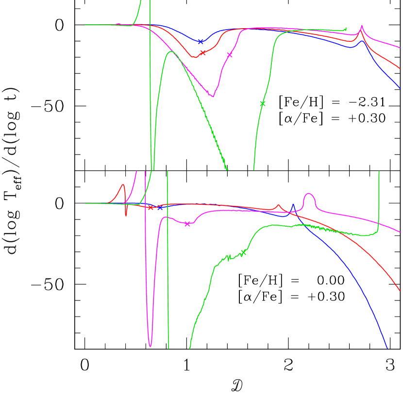
Figure 6: The derivative d$(\log T_{\rm eff})$/d$(\log t)$ is plotted as a function of distance along an evolutionary track for the abundances shown. The distance is calculated from ${\cal D}=\sum\Delta{d}$ where $\Delta{d}=[1.25\,(\Delta\log L)^{2}+10.0\,(\Delta\log T_{\rm eff})^{2}]^{1/2}$ with ${\cal D}=0.0$ at the lowest mass point on the isochrone; see BV01.) In the upper panel, the derivatives plotted correspond to those for 0.9 (blue), 1.1 (red), 1.5 (magenta) and $1.8{\cal M}_{\odot}$ (green) tracks; in the lower panel, the derivatives correspond to 0.9 (blue), 1.4 (red), 1.8 (magenta), and $2.4{\cal M}_{\odot}$ (green) tracks. The adopted location of the HZGP point is indicated by the symbol ${\bf\times}$ on each curve.

Consider first the morphology of the temperature derivative in the metal-poor tracks illustrated in the upper panel of Figure 6. On the $0.9{\cal M}_{\odot}$ track, the Hertzsprung gap point (HZGP) is easily identifiable at the local derivative minimum. However, on the $1.1{\cal M}_{\odot}$ track, the development of apparently anomalous morphology at the HZGP derivative minimum occurs even before the incipient blue hook becomes evident in the $1.5{\cal M}_{\odot}$ track, on which the morphology of the minimum is obviously different from that of the $0.9{\cal M}_{\odot}$ track. The fully developed blue hook is clearly evident in the $1.8{\cal M}_{\odot}$ track, which also shows a more extreme version of the transition to the giant branch. These differences imply that the the minima do not correspond to equivalent evolutionary phases: in the low-mass regime, the minimum is an artifact of the rather diffuse pp-chain processing in the hydrogen-burning core, whereas in the high-mass regime, it is an artifact of the more centrally concentrated CNO cycle processes (due to their much higher temperature sensitivity) that dominate the energy production. The primary EEPs at the Hertzsprung gap and near the base of the RGB (BRGB) bracket the bottom of the giant branch on the $0.9{\cal M}_{\odot}$ track; the equivalent HZGP point on the higher mass tracks is found at the inflection point in the derivative on the following side of the minimum.

The lower panel of Figure 6 illustrates that, in metal-rich grids, the transition occurs in a distinctly different way. In this instance, the well-defined derivative minimum in the $1.8{\cal M}_{\odot}$ track, does correspond to the HZGP EEP located at the local minimum in the $0.9{\cal M}_{\odot}$ track; the corresponding primary EEP in the $2.4{\cal M}_{\odot}$ track is the inflection point marked on the following edge.

One other adjustment that had to be made to the interpolation scheme was to manage the transition from stubby giant branches in the tracks of the more massive stars, which terminate near the location of the evolutionary pause (GBPS) that occurs when the H-burning shell contacts the chemical composition discontinuity caused by the first dredge-up, to fully developed RGBs in the lower mass tracks. This was accomplished by making the GBPS primary EEP degenerate with the RGB tip EEP for those tracks with stubby RGBs, such as the $1.8{\cal M}_{\odot}$ track illustrated in the upper panel of Figure 6, and in the $2.4{\cal M}_{\odot}$ track in the lower panel.

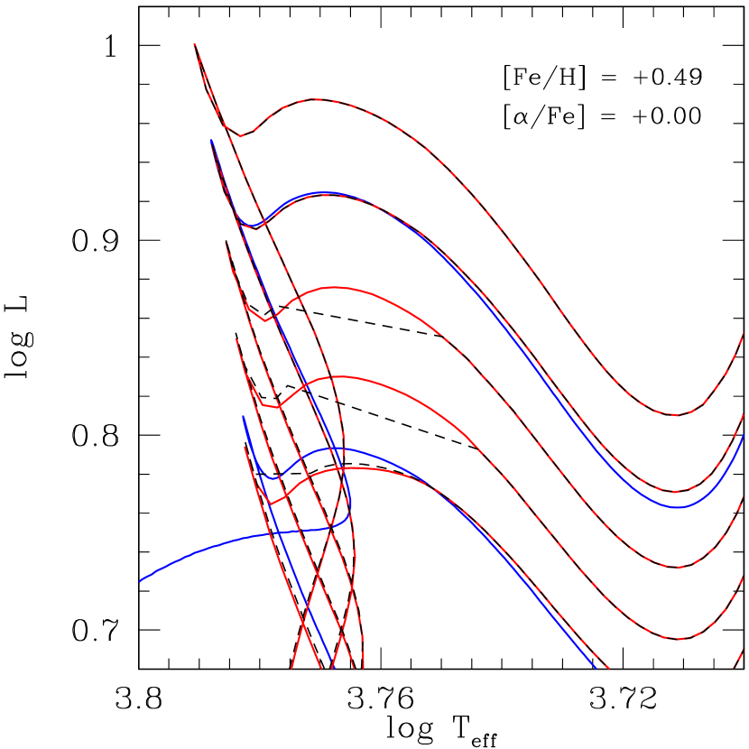
Figure 7: The central H exhaustion and subgiant segments of the evolutionary sequences for 1.4 and $1.5{\cal M}_{\odot}$ stars with the indicated abundances are plotted (solid blue lines) along with several isochrones. The dashed black lines represent the isochrones interpolated via the Akima spline for the ages 2.6, 2.8, 3.0, 3.2, and 3.4 Gyr; the solid red lines represent the same isochrones obtained via linear interpolation. The straight line segments just past the blue ends of the hook in the 3.0, 3.2, and 3.4 Gyr isochrones that were obtained using the Akima spline (the dashed black lines) indicate the existence of gaps in the point distributions. They correspond to mass differences of slightly more than $0.001{\cal M}_{\odot}$.

In Bergbusch & VandenBerg (1992), it was clearly demonstrated that linear interpolation works extremely well with the prescribed set of primary EEPs defined therein in the regime of low-mass stars. In BV01, Akima spline interpolation was introduced primarily to improve the calculation of isochrone probability functions (IPFs), luminosity functions, and color functions. However, in preparing the current set of grids, we noticed that isochrones in the age range of $\approx 2.8$–3.4 Gyr, derived via spline interpolation, occasionally exhibited gaps in the point distribution over the transition from the blue hook to the base of the RGB. As illustrated in Figure 7, the same isochrones derived via linear interpolation do not have these gaps. Our interpretation of this is that, even though the EEP Mass-Age relations defined by the primary and secondary EEPs at their locations on the evolutionary tracks remain monotonic, very small wobbles of the spline (corresponding to slightly more than $0.001{{\cal M}_{\odot}}$, at most) create “forbidden” regions in the interpolation relations between the tracks (i.e., zones where the age increases slightly with increasing mass). (Isochrone points interpolated by the two methods occupy slightly different locations only because of differences in the shape of the Mass–Age relations in the regions between the tracks. In both cases, the Akima spline was used to interpolate $\log L$ and $\log T_{\rm eff}$ between the tracks.)

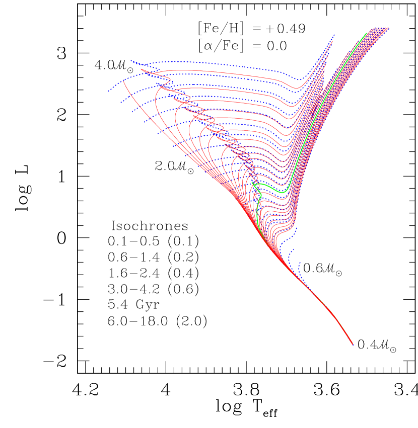
Figure 8: The complete grid of evolutionary tracks for the scaled solar, [Fe/H]$=+0.49$ grid are plotted with the dotted blue lines. The tracks are plotted at $0.1{\cal M}_{\odot}$ intervals from 0.4 up to $2.0{\cal M}_{\odot}$, then at $0.2{\cal M}_{\odot}$ intervals up to $2.4{\cal M}_{\odot}$, and at $0.3{\cal M}_{\odot}$ intervals up to $3.6{\cal M}_{\odot}$. There is an additional track at $1.031{\cal M}_{\odot}$, which is the transitional mass at which the blue hook appears. The grid is completed with a $4.0{\cal M}_{\odot}$ track. The isochrones span the range of ages from 0.1 to 18.0 Gyr (as indicated). Those plotted with solid red lines were derived via spline interpolation; the single green isochrone, with an age of 3 Gyr, was derived via linear interpolation.

The complete grid of evolutionary sequences from which the segments of the 1.4 and $1.5{{\cal M}_{\odot}}$ tracks plotted in the figure just discussed were taken is shown in Figure 8. Note that the spacing in mass is quite fine, as a total of 25 tracks span the range in mass from 0.4 to $4.0{{\cal M}_{\odot}}$. This includes one track for $1.031{{\cal M}_{\odot}}$, which is the mass (for this particular grid) at which a transition is made between stars that have radiative cores at central H exhaustion to those that maintain convective cores throughout the MS phase. (As a consequence of this transition, higher mass tracks have blueward hooks at their turnoffs.) Also plotted are several isochrones to illustrate both the range in age for which isochrones may be computed (0.2–18 Gyr) and the approximate region in the H–R diagram where they are obtained using linear interpolation to avoid the problem described in the preceding paragraph (i.e., in the vicinity of the 3.0 Gyr isochrone, which has been plotted in green). The main signatures of CCO are (i) a widening of the main-sequence band (the region between the ZAMS and the line connecting the red ends of the hook feature on each of the higher mass tracks), and (ii) a decrease in the mass at which a transition is made from an extended to a stubby RGB. In this particular grid, it occurs at $\approx 1.8{{\cal M}_{\odot}}$.

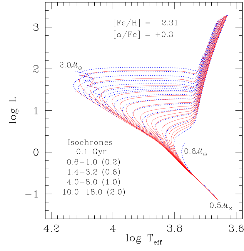
Figure 9: The complete grid of evolutionary tracks for the [Fe/H]$=-2.31$, $[\alpha/{\rm Fe}]=+0.3$ grid are plotted with the dotted blue lines. The tracks are spaced at $0.1{\cal M}_{\odot}$ intervals with an additional track at ${1.44\cal M}_{\odot}$, which is the transitional mass for the development of the blue hook. The isochrones, plotted as solid red lines, span the range of ages from 0.1 to 18.0 Gyr, as indicated.

All of the “VRSS” grids (see Table 2) encompass the same ranges in mass and age as that shown in Fig. 8. In the case of the grids that have been computed for [$\alpha$/Fe] $=0.0,0.3,$ and 0.6 (see Table 1), tracks have been computed from $0.5{{\cal M}_{\odot}}$ to that mass (within the range $2.0\leq{{\cal M}_{\odot}}\leq 2.2$) which enables isochrones to be computed down to $\sim 1$ Gyr. An example of the latter is given in Figure 9, which illustrates the evolutionary sequences that comprise the “VR2A-231” grid (i.e., that for [$\alpha$/Fe] $=0.3$ and [Fe/H] $=-2.31$), along with representative isochrones. Note that the transition between stars with, and without, blueward hooks at their turnoffs occurs at a much higher mass ($1.44{{\cal M}_{\odot}}$) than in the grid plotted in the previous figure.

4 Observational Tests of the Stellar Models

4.1 Metal-Deficient Star Clusters

In principle, the many young, metal-poor star clusters that populate the Large Magellanic Cloud (LMC) should provide especially tight constraints on the extent of overshooting in low-metallicity stars. However, in practice, this is not yet possible, mainly because current estimates of their chemical compositions are so uncertain. For instance, even though very well-defined CMDs are now available for NGC 2155, NGC 2173, and SL 556 (see Gallart et al. 2003), it is not at all clear which models should be compared with the photometric data when current [Fe/H] determinations for each of these systems vary by about 0.6 dex (typically from [Fe/H] $\sim-1.2$ to $\sim-0.6$; see the review of the properties of these clusters by Bertelli et al. 2003). All that one can reasonably do, until this situation improves, is ascertain whether it is possible to find an isochrone (or generate a synthetic CMD) that does a satisfactory job of matching an observed CMD on the assumption of a reddening, distance, and metal abundance within the ranges of their uncertainties. This is effectively what was done by Bertelli et al. and by Woo et al. (2003) in their studies of NGC 2155, NGC 2173, and SL 556.

How well are our isochrones able to fit the CMDs of these three clusters? It is certainly of some interest to know the answer to this question — and, as shown below, our models appear to fare quite well. Our approach is to adopt the line-of-sight reddenings from the Schlegel, Finkbeiner, & Davis (1998) dust maps and to assume, as a first approximation, that all three systems are at a distance corresponding to $(m-M)_{0}=18.50$, which is very close to the mean LMC modulus that has been derived using many different techniques (e.g., see Benedict et al. 2002). Having set the reddening and distance, there are no free parameters other than the metallicity (and age). The latter can be “determined” simply by overlaying the isochrones for different chemical compositions and ages onto an observed CMD and then selecting that isochrone which most closely matches the observations. (The metal abundance obtained in this way is obviously nothing more than a “prediction” and, as such, of limited usefulness only when, as in the case of the LMC clusters, metallicities are poorly known.) The result of this exercise is shown in Figure 10 and in the left-hand panel of Figure 11. [Note that $E(V-R)=0.59\,E(B-V)$ has been assumed; see, e.g., Bessell et al. (1998). Furthermore, [$\alpha$/Fe] $=0.3$ has been adopted simply because such an enhancement has been found in the majority of stars in the Milky Way with [Fe/H] $\mathrel{\hbox{\raise 2.58334pt\hbox{$<$}\kern-7.74998pt\lower 2.15277pt\hbox{$\sim$}}}-0.6$, whether in globular clusters (e.g., Carney 1996; Kraft et al. 1998) or in the field (e.g., Zhao & Magain 1990; Nissen & Schuster 1997). The accuracy of this assumption for the three LMC clusters considered has not yet been established.]

The level of agreement between theory and observations is actually surprisingly good (and quite comparable to the findings of Bertelli et al. 2003; Woo et al. 2003). [The most obvious discrepancy is the failure of the isochrones to match the $V-R$ colors of the upper RGB stars in NGC 2173 and SL 556. This may indicate that the inferred metallicities and/or distances should be revised slightly or that there is a problem with the model temperatures and/or the $(V-R)$–$T_{\rm eff}$ relations that we have used (from VC03) to transpose the isochrones to the observed plane. In fact, there is already some evidence to suggest that the $V-R$ colors given by the VC03 transformations are too blue for low-gravity stars — see the study of NGC 188 by VandenBerg & Stetson (2004). However, until the observational parameters are placed on a firmer footing, it would be premature to conclude that the latter explanation is the correct one. NGC 2155 would not show a similar mismatch between the predicted and observed giant branch if, e.g., the adopted distance or metallicity was too high. The fact that the MS segment of the isochrone used to fit the observations is too red does provide some indication that a lower metal abundance may be more appropriate, but we have found that our models for [Fe/H] $=-1.01$, which is the next lowest metallicity in our grids, are too blue. This suggests some preference for models with [Fe/H] $\sim-0.9$.]

The inferred [Fe/H] values are all well within the ranges of uncertainty encompassing current photometric and spectroscopic metallicity estimates and, in fact, are close to the metal abundances deduced or assumed by Bertelli et al. and Woo et al. Even our derived ages are similar to those found by the latter: what differences exist can be attributed mostly to the different assumptions that have been made regarding the cluster reddenings and distances. Indeed, until much tighter constraints are placed on the cluster metal abundances, it is not possible to say whose interpretations of the observed CMDs are the most accurate ones. Certainly, from our perspective, it is very encouraging that NGC 2155, NGC 2173, and SL 556 do not appear to pose any serious difficulties for the isochrones presented in this investigation, which is really the main point of including a brief analysis of data for these systems in this investigation.

A much better test of the overshooting models is provided by the metal-poor Galactic cluster NGC 2243. Fortunately, Anthony-Twarog, Atwell, & Twarog (2005) have just carried out a very thorough analysis of $uvby\,Ca\,H_{\beta}$ photometry for this system, from which they found $E(B-V)=0.055$ and [Fe/H] $=-0.57$. Their reddening estimate is consistent with that derived from the Schlegel et al. (1998) dust maps, which give $E(B-V)=0.074$. As Anthony-Twarog et al. point out, the latter provides a line-of-sight upper limit, though it should be close to the value appropriate for NGC 2243 given that this cluster lies above the Galactic plane. Moreover, from their examination of the work that has been carried out on this cluster to date, they suggest that both photometric and spectroscopic metallicity determinations seem to be converging to an [Fe/H] value of $\approx-0.55\pm 0.1$.

As illustrated in the right-hand panel of Fig. 11, an overshooting isochrone for 3.1 Gyr, [Fe/H] $=-0.61$, and [$\alpha$/Fe] $=0.3$ provides an excellent match to the CMD obtained by Bergbusch, VandenBerg, & Infante (1991). This metallicity differs from the Anthony-Twarog et al. (2005) best estimate by $<0.1$ dex, and the assumed reddening is approximately midway between the $E(B-V)$ value derived by Anthony-Twarog et al. and that from the Schlegel et al. (1998) dust maps. Insofar as the $\alpha$-element abundances are concerned, Gratton & Contarini (1994) obtained [$\alpha$/Fe] $\approx 0.1$ (if [Fe/H] $=-0.48$) from high resolution spectroscopy of two cluster giants. The adoption of an iron abundance lower by $\sim 0.1$ dex would imply an increase in the [$\alpha$/Fe] value by the same amount. Importantly, Gratton & Contarini have concluded that a scaled-solar composition is not favored by their data. Indeed, they do not find any significant differences in the chemical compositions of NGC 2243 and field stars of the same [Fe/H].

One could, of course, get similar fits of isochrones to the observed CMD on the assumption of slightly lower or higher reddenings, but the derived distance moduli from the main-sequence fitting technique and the ages would also differ slightly. (Our impression is that the best match to the observations is obtained for the adopted parameter values.) NGC 2243 provides an especially important check of our calibration of $F_{\rm over}$ because it is a sufficiently old cluster that the upper MS stars have masses in the range where the overshooting parameter is a strong function of mass. The fact that the models are able to reproduce the morphology of the cluster turnoff so well provides good support for our $F_{\rm over}$–mass–metallicity relation.

4.2 The Binary TZ Fornacis

TZ For is one of a very small group of binaries with sufficiently well-determined masses, radii, effective temperatures, and metal abundances that they provide stringent tests of stellar models. Indeed, it has proven to be especially difficult for computed models, even those that allow for convective overshooting, to match the properties of TZ For (see Andersen et al. 1991; and, in particular, Lastennet & Valls-Gabaud 2002). According to Andersen et al., the components of this binary have masses of $1.95\pm 0.03$ and $2.05\pm 0.06{{\cal M}_{\odot}}$, radii of $3.96\pm 0.09$ and $8.32\pm 0.12{{\cal R}_{\odot}}$, and effective temperatures corresponding to $\log T_{\rm eff}=3.803\pm 0.007$ and $3.699\pm 0.009$, respectively. They also obtained [Fe/H] $=-0.1\pm 0.1$ from a direct spectroscopic determination of its metal abundance.

TZ For played no role in the calibration of the overshooting parameter, $F_{\rm over}$, so it is particularly pleasing to find that our models are able to provide quite a satisfactory fit to its components. The locations of these stars are plotted in Figure 12 on the ($M_{\rm bol},\,\log T_{\rm eff}$)–plane, together with evolutionary tracks that have been computed for the observed masses and two different metallicities, [Fe/H] $=0.0$ and $+0.13$. Taken at face value, the models suggest that the fainter component has a metal abundance close to [Fe/H] $=+0.06$, which is well within the uncertainty of the spectroscopically determined metallicity. If the actual iron abundance is somewhat higher or lower than this value, one could still obtain a precise fit to the luminosity and temperature of this star by adopting a helium abundance that differs somewhat from the assumed values (see Table 2).

According to the models, the $1.95{{\cal M}_{\odot}}$ star is nearing the end of its main-sequence phase, with an age in the range of 1.26 Gyr (if [Fe/H] $=0.0$) to 1.33 Gyr (if [Fe/H] $=+0.13$). Its companion is predicted to have an age at its observed luminosity between 1.12 and 1.19 Gyr (assuming [Fe/H] $=0.0$ and $+0.13$, respectively) if it is a first-ascent red-giant-branch star. Their ages are not in perfect agreement, but the uncertainties in their masses, though small, are still large enough that identical ages could almost certainly be found for both stars if their masses are more nearly equal than observed (and remain within the observed $1\sigma$ mass limits). More likely is the possibility that the most massive component is in the core He-burning phase (see the discussion by Andersen et al. 1991), in which case there may not be an age problem. (Unfortunately, we do not yet have the means to test this hypothesis, but it goes without saying that the probability of finding a binary like TZ For is much higher if both of its components are in long-lived evolutionary phases.) In any case, we conclude from our analysis of this binary that an amount of overshooting equivalent to $F_{\rm over}\approx 0.55$ is required to model $\sim 2{{\cal M}_{\odot}}$ stars having metallicities close to that of the Sun.

4.3 Globular Cluster Giant Branches

Vandenberg et al. (2000) have already shown that their computed giant branches for $\sim 0.8{{\cal M}_{\odot}}$ metal-poor stars are in good agreement with those derived for Galactic globular clusters (GCs) on the $(\log T_{\rm eff},\,M_{\rm bol})$–plane by Frogel, Persson, & Cohen (1981) using infrared photometry. Moreover, BV01 have found that there is good consistency between the models and the $V-I,\,I$ RGB fiducials for several GCs that were determined by Da Costa & Armandroff (1990), if Schlegel et al. (1998) reddenings and distance moduli based on zero-age horizontal-branch (ZAHB) models are assumed. A very similar plot to that provided in the latter study is given in Figure 13, except that a wider range in [Fe/H] is considered and the recent determination by Bellazzini, Ferraro, & Pancino (2001) of the absolute $I$ magnitude of the RGB tip ($M_{I}^{\rm TRGB}$) of $\omega$ Centauri is shown (the open square). Their estimate of $M_{I}^{\rm TRGB}=4.04\pm 0.12$, which is based on extensive cluster photometry and the distance to $\omega$ Cen obtained by Thompson et al. (2001) from a detached eclipsing binary, provides the most accurate empirical zero-point for the $M_{I}^{\rm TRGB}$–[Fe/H] relationship that is currently available.

For the sake of clarity, the open square has been located at $(V-I)_{0}=1.48$, which is very close to the color of RGB tip stars having [Fe/H] $=-1.71$, according to the relation between $(V-I)_{0}^{\rm TRGB}$ and [Fe/H] determined by Bellazzini et al. (2001). (This will depend on the particular metallicity scale which is assumed.) Importantly, the absolute $I^{\rm TRGB}$ magnitudes predicted by the metal-poor isochrones plotted in Fig. 13 (indeed, by those for all [Fe/H] values less than $\sim-0.8$) agree very well with the empirical derivation of $M_{I}^{\rm TRGB}$. Comparable agreement is also found for the absolute $I^{\rm TRGB}$ magnitudes of M 15, NGC 6752, and NGC 1851 when distances based on VandenBerg et al. (2000) ZAHB loci are assumed (see VandenBerg 2000). This consistency adds to the support for these particular HB models found from recent studies of the pulsational properties of RR Lyraes in GCs (see De Santis & Cassisi 1999; Cacciari, Corwin, & Carney 2005). In fact, the ZAHB-based distance modulus for NGC 6752 is nearly identical with that derived from its white dwarfs by Renzini et al. (1996); specifically, $(m-M)_{V}=13.22\pm 0.1$ if $E(B-V)=0.056$ and $A_{V}=3.1\,E(B-V)$.

The absolute $I^{\rm TRGB}$ magnitude of 47 Tuc is slightly fainter than those of the other GCs considered in Fig. 13, but this is implied by several of the latest distance determinations. In particular, Zoccali et al. (2001) obtained $(m-M)_{V}=13.27\pm 0.14$ from the cluster white dwarfs, while the fit of the main-sequence of 47 Tuc to that defined by local Population II subdwarfs by Grundahl, Stetson, & Andersen (2002) yielded $(m-M)_{V}=13.33\pm 0.04\pm 0.1$. (Note that our estimate of the distance modulus of 47 Tuc assumes that the cluster has [Fe/H] $=-0.83$: if this were increased to $-0.71$, the ZAHB-based modulus would decrease to 13.30.) One possible implication of these results is that the variation of $M_{I}^{\rm TRGB}$ with [Fe/H] at higher metal abundances may be slightly steeper than that found by Bellazzini et al. (2001; their equation 4).

Perhaps the main concern with Fig. 13 is that the cluster metallicities, as inferred from the isochrones, tend to be on the low side of most estimates (see Table 3). It is not clear that this is necessarily a problem with the models, but it is certainly possible that either the predicted temperatures are too cool or the predicted colors are too red. Although, as noted above, the model $T_{\rm eff}$ scale is consistent with that derived for GCs from $V-K$ photometry, the uncertainties in the empirically determined temperatures are $\sim\pm 100$ K. This is easily more than enough to reconcile the models with the latest spectroscopic abundances for several of the clusters.

For instance, very close to the [Fe/H] values determined by Kraft & Ivans (2003) for NGC 6752, NGC 1851, and 47 Tuc would be implied by the superposition of the cluster fiducials onto the isochrones if the temperatures of the latter were increased by only 70 K. (Somewhat larger adjustments would be needed if the most accurate metallicities are those by Carretta & Gratton 1997). The difficulty with this solution is that the implied metallicity of M 15 would be $\approx-2.1$, in conflict with their spectroscopic value of $-2.42$ (see Table 3). Without any justification for doing so, it would not be very satisfying to correct the temperatures of the isochrones for some metal abundances, but not for others.

A more optimistic comment on the comparison between theory and observations presented in Fig. 13 is that the predicted [Fe/H] scale is consistent with that derived by Zinn & West (1984) to within $\approx 0.15$ dex. This is comparable to, if not smaller than, the uncertainties associated with most [Fe/H] determinations at the present time (e.g., compare the results listed in Table 3). Needless to say, it is going to be very difficult to say whether or not the colors derived from the VC03 color–$T_{\rm eff}$ relations are too red until much tighter constraints are placed on [Fe/H] and temperature measurements. Fortunately, model colors do not play a critical role in the interpretation of the CMDs for simple stellar populations, like open and globular star clusters. It is mainly to address the observations of those systems that have complicated star formation and chemical evolution histories (e.g., the LMC, dwarf spheroidal galaxies) that some calibration of the model colors is necessary (see the fairly extensive discussion of this matter by VandenBerg 2005).

We conclude this section with another example to show how well our isochrones, in conjunction with the VC03 color transformations, are able to reproduce extended RGBs; in this case, that of the metal-rich Bulge globular cluster, NGC 6528. To produce the plot shown in Figure 14, the observations of NGC 6528 obtained by Richtler et al. (1998) were tranposed to the [$(V-I)_{0},\,M_{V}$]–plane in the following way. First, the observed $V$ magnitudes were converted to absolute $V$ magnitudes by assuming that the cluster HB clump stars have a mean $M_{V}\approx 0.9$. This should be accurate to within $\pm 0.15$ mag for a GC having [Fe/H] $\approx-0.1$ (Zoccali et al. 2004) since, for instance, this is close to the mean $M_{V}$ of the HB stars in the younger, but slightly more metal rich, open cluster M 67 (see Fig. 3). Having set the $M_{V}$ scale, the reddening, $E(V-I)=0.62$, then follows from the horizontal shift between the observed $V-I$ colors and those predicted for the lower RGB portion of an isochrone for the cluster metallicity; i.e., that part which is fainter than the HB. (Because the location of the giant branch is not a very sensitive function of the assumed age, any isochrone within the range of, say, 8 to 16 Gyr could be used.)

This assumes that the models (for [Fe/H] $\approx 0.0$) are reliable, but there is ample justification for such an assumption. For one thing, the predicted $T_{\rm eff}$ scale has been precisely normalized using the Sun. For another, as shown by VC03, their color transformations are in excellent agreement with the best available empirical color–$T_{\rm eff}$ relations for dwarfs and giants, as well as with observed color–color diagrams. (Models for near solar metallicities are much more secure than those for metal-deficient or super-metal-rich stars.)

If $E(V-I)=1.33\,E(B-V)$, as assumed by Zoccali et al (2004; see Dean, Warren & Cousins 1978), then our estimate of $E(V-I)$ corresponds to $E(B-V)=0.47$, which is in very good agreement with the value adopted by Zoccali et al. ($0.46\pm 0.04$). Be that as it may, the main point that we wish to make here is that the upper RGB segment of the isochrone plotted in Fig. 14 provides quite a reasonable fit to the cluster giants all the way to $(V-I)\approx 4.0$. (As the metallicity is uncertain by at least $\pm 0.2$ dex, it is easy to obtain an even more extended RGB simply by assuming a slightly higher metal abundance. Recall that the $V-I$ colors and the bolometric corrections relevant to cool stars are extremely sensitive functions of temperature; see VC03). Thus, to within the uncertainties of the many factors at play, our computations do a satisfactory job of reproducing the giant branches of Galactic GCs over the entire range of their metallicities.

Despite the encouraging agreement of our models with observations (also see VandenBerg et al. 2000; BV01, VC03, Clem et al. 2004), it should be kept in mind that the uncertainties associated with “observed” temperatures, chemical compositions, and distances, as well as the photometric data themselves (see VandenBerg 2005), permit considerable latitute in the models. Indeed, coupled with our poor understanding of, in particular, convection in stellar envelopes and the physical process (or processes) that are apparently operating to inhibit diffusion in GC stars, one should not expect, e.g., perfect agreement between synthetic and observed CMDs.

5 Conclusions

This investigation presents a total of 72 grids of stellar evolutionary tracks along with the software needed to generate isochrones for any age within the ranges encompassed by the tracks, and to predict the numbers of stars along them (isochrone probability functions, LFs, CFs). This includes 60 grids in which enhancements in the $\alpha$-elements are treated explicitly; i.e., for each of 20 [Fe/H] values between $-2.31$ and $0.0$, model sequences are provided for [$\alpha$/Fe] $=0.0,0.3$, and 0.6. In each of these cases, isochrones extending to the RGB tip may be computed for ages from 1 to 18 Gyr. The remaining 12 grids are for [Fe/H] values from $-0.60$ to $+0.49$, on the assumption of [$\alpha$/Fe] $=0.0$ (in each case) and ranges in mass that are sufficient to permit the calculation of isochrones down to 0.2 Gyr.

Diffusive processes have not been considered in these computations. In fact, as discussed in §3, models that take diffusion into account are not able to explain either the spectroscopic data or the photometric observations of old star clusters as well as those that neglect this physics. (As already mentioned, it is generally thought that there are competing processes at work in the surface layers of stars that limit the efficiency of diffusion. However, our understanding is still in a fairly primitive state.) The novel feature of the present models is that convective core overshooting has been treated using a parameterized form of the Roxburgh criterion, in which the free parameter, $F_{\rm over}$, is assumed to be a function of both mass and metal abundance. All of the tests that we have conducted thusfar (including those considered by P. D. Dowler & D. A. VandenBerg, in preparation) support our calibration of $F_{\rm over}$. Indeed, our overshooting models are able to reproduce the turnoff morphologies of cluster CMDs very well, irrespective of their age and metallicity. They also satisfy the constraints provided by the binary TZ For, which has proven to be especially difficult for non-overshooting and overshooting computations to date (see Lastennet & Valls-Gabaud 2002). (The data for several other binaries and open clusters are examined in detail by Dowler & VandenBerg, who also compare the present models with overshooting calculations in which convective cores are extended by some fraction of a pressure scale-height.) It is our intention to extend the models in the coming year to include, in particular, the core He-burning phase.

Figure 1: The variation of $F_{\rm over}$ with mass that has been assumed in the computation of evolutionary tracks for stars having the indicated chemical abundances.

Figure 2: Plot, as a function of $\log Z$, of the mass at which a transition is made between lower mass stars, on the one hand, and higher mass stars, on the other, that have radiative and convective cores, respectively, when they reach the end of the main-sequence phase. These results are based on the “VRSS” grids discussed in §3, which were computed for values of $Z$ in the range $0.005\leq Z\leq 0.05$. (Although not shown, similar loci were computed for the sets of tracks having [Fe/H] values from $-2.31$ to 0.0 and [$\alpha$/Fe] $=0.0$, 0.3, and 0.6.)

Figure 3: Main-sequence fit of a 4.0 Gyr isochrone for [Fe/H] $=-0.04$ to the $BV$ photometry of M 67 by Montgomery et al. (1993), on the assumption of the indicated reddening and apparent distance modulus.

Figure 4: Main-sequence fit of a 1.75 Gyr isochrone for [Fe/H] $=-0.04$ to the $VI$ photometry of NGC 7789 by Gim et al. (1998), on the assumption of the indicated reddening and apparent distance modulus.

Figure 5: Main-sequence fit of a 2.4 Gyr isochrone for [Fe/H] $=0.0$ to the $BV$ photometry of NGC 6819 by Rosvick & VandenBerg (1998), on the assumption of the indicated reddening and apparent distance modulus.

Figure 10: Overlay of those isochrones for the indicated [Fe/H] values and ages that best reproduce the CMDs of the LMC clusters NGC 2173 and SL 556 (Gallart et al. 2003) on the assumption of the reddening and apparent distance modulus given in the upper left-hand corner of each panel (see the text). The abundances of the $\alpha$-elements are assumed to be enhanced by [$\alpha$/Fe] $=0.3$.

Figure 11: Similar to the previous figure, except that isochrones are compared with Gallart et al. (2003) $VR$ observations of NGC 2155 (left-hand panel), also in the LMC, and with $BV$ photometry for the Galactic open cluster NGC 2243 (right-hand panel) by Bergbusch et al. (1991). In the latter case, the adopted distance modulus was derived from a main-sequence fit of the observed CMD to the models on the assumption of the indicated reddening (see the text). In both cases, enhanced abundances of the $\alpha$-elements by [$\alpha$/Fe] $=0.3$ has been assumed.

Figure 12: Comparison of computed evolutionary tracks for the observed masses of TZ Fornacis and for metallicities [Fe/H]$=0.0$ (solid curves) and $+0.13$ (dashed curves) with the observed parameters of the binary (filled circles and $1\sigma$ error parallelograms) obtained by Anderson et al. (1998). From spectroscopic observations of TZ For, the latter determined an [Fe/H]$=+0.1\pm 0.1$. (A parallelogram is a more accurate representation of the error boxes than a rectangle, as is often used, because the uncertainty in $M_{\rm bol}$ at a given $\log T_{\rm eff}$ is due only to the uncertainty in the stellar radius.)

Figure 13: Overlay of the fiducial sequences derived by Da Costa & Armandroff (1990) for M 15, NGC 6752, NGC 1851, and 47 Tucanae, on the assumption of the indicated reddenings and apparent distance moduli, onto the giant-branch segments of 13 Gyr isochrones for [Fe/H] values ranging from $-2.31$ to $-0.40$, assuming [$\alpha$/Fe] $=0.3$ in each case. Note that, as shown by VandenBerg (2000), turnoff ages close to 13 Gyr are consistent with the adopted $(m-M)_{V}$ values only for M 15 and NGC 6752: somewhat younger ages ($\approx 11.5$ Gyr) are obtained for NGC 1851 and 47 Tuc. The large open square, with error bars, gives the absolute $I$ magnitude of the RGB tip stars in $\omega$ Centauri determined by Bellazzini et al. (2001); see the text.

Figure 14: Comparison of a 12 Gyr isochrone for [Fe/H] $=-0.11$ and [$\alpha$/Fe] $=0.0$ with the CMD of NGC 6528 by Richtler et al. (1998) when the indicated values of $E(V-I)$ and $(m-M)_{V}$ are assumed. The adopted metal abundances are close to those derived by Zoccali et al. (2004), who obtained [Fe/H] $=-0.1$ and [$\alpha$/Fe] values between 0.0 (for Ca, Ti) and 0.1 (for O, Mg, Si) from their spectroscopic study of NGC 6528.

Table 1: Initial Chemical Abundances for the VR0A, VR2A, and VR4A Grids of Stellar Models that have [$\alpha$/Fe] $=0.0,0.3,$ and 0.6, respectively

			[$\alpha$/Fe] $=0.0$			[$\alpha$/Fe] $=0.3$			[$\alpha$/Fe] $=0.6$
[Fe/H]	$Y$		$Z$	File Name		$Z$	File Name		$Z$	File Name
$-2.31$	0.2352		1.000E$-04$	vr0a-231		1.690E$-04$	vr2a-231		3.070E$-04$	vr4a-231
$-2.14$	0.2353		1.500E$-04$	vr0a-214		2.540E$-04$	vr2a-214		4.610E$-04$	vr4a-214
$-2.01$	0.2354		2.000E$-04$	vr0a-201		3.380E$-04$	vr2a-201		6.140E$-04$	vr4a-201
$-1.84$	0.2356		3.000E$-04$	vr0a-184		5.070E$-04$	vr2a-184		9.210E$-04$	vr4a-184
$-1.71$	0.2358		4.000E$-04$	vr0a-171		6.760E$-04$	vr2a-171		1.230E$-03$	vr4a-171
$-1.61$	0.2360		5.000E$-04$	vr0a-161		8.450E$-04$	vr2a-161		1.540E$-03$	vr4a-161
$-1.53$	0.2362		6.000E$-04$	vr0a-153		1.014E$-03$	vr2a-153		1.840E$-03$	vr4a-153
$-1.41$	0.2366		8.000E$-04$	vr0a-141		1.352E$-03$	vr2a-141		2.450E$-03$	vr4a-141
$-1.31$	0.2370		1.000E$-03$	vr0a-131		1.690E$-03$	vr2a-131		3.070E$-03$	vr4a-131
$-1.14$	0.2380		1.500E$-03$	vr0a-114		2.540E$-03$	vr2a-114		4.610E$-03$	vr4a-114
$-1.01$	0.2390		2.000E$-03$	vr0a-101		3.380E$-03$	vr2a-101		6.140E$-03$	vr4a-101
$-0.83$	0.2410		3.000E$-03$	vr0a-083		5.060E$-03$	vr2a-083		9.150E$-03$	vr4a-083
$-0.71$	0.2430		4.000E$-03$	vr0a-071		6.750E$-03$	vr2a-071		1.220E$-02$	vr4a-071
$-0.61$	0.2450		5.000E$-03$	vr0a-061		8.430E$-03$	vr2a-061		1.520E$-02$	vr4a-061
$-0.52$	0.2470		6.000E$-03$	vr0a-052		1.010E$-02$	vr2a-052		1.820E$-02$	vr4a-052
$-0.40$	0.2510		8.000E$-03$	vr0a-040		1.345E$-02$	vr2a-040		2.410E$-02$	vr4a-040
$-0.30$	0.2550		1.000E$-02$	vr0a-030		1.676E$-02$	vr2a-030		2.991E$-02$	vr4a-030
$-0.20$	0.2600		1.250E$-02$	vr0a-020		2.090E$-02$	vr2a-020		3.715E$-02$	vr4a-020
$-0.11$	0.2645		1.500E$-02$	vr0a-011		2.500E$-02$	vr2a-011		4.425E$-02$	vr4a-011
$0.00$	0.2715		1.880E$-02$	vr0a000		3.125E$-02$	vr2a000		5.490E$-02$	vr4a000

Table 2: Initial Chemical Abundances for the VRSS Grids of Stellar Models that have Scaled-Solar Abundances of the Heavy Elements

[Fe/H]	$Y$	$Z$	File Name
$-0.60$	0.24644	0.0050	vrss-060
$-0.52$	0.24864	0.0060	vrss-052
$-0.39$	0.25304	0.0080	vrss-039
$-0.29$	0.25744	0.0100	vrss-029
$-0.19$	0.26294	0.0125	vrss-019
$-0.11$	0.26844	0.0150	vrss-011
$-0.04$	0.27350	0.0173	vrss-004
$+0.00$	0.27680	0.0188	vrss000
$+0.13$	0.29044	0.0250	vrss013
$+0.23$	0.30144	0.0300	vrss023
$+0.37$	0.32344	0.0400	vrss037
$+0.49$	0.34544	0.0500	vrss049

Table 3: Globular Cluster [Fe/H] Determinations from Different Sources

Name	Zinn & West (1984)	Carretta & Gratton (1997)	Kraft & Ivans (2003)
M 15	$-2.15$	$-2.12$	$-2.42$
NGC 6752	$-1.54$	$-1.42$	$-1.57$
NGC 1851	$-1.36$	$\ldots$	$-1.19$
47 Tuc	$-0.71$	$-0.70$	$-0.70$

References

- Andersen (1991) Andersen, J. 1991, A&AR, 3, 91
- Andersen et al. (1991) Andersen, J., Clausen, J. V., Nordström, B., Tomkin, J., & Mayor, M. 1991, A&A, 246, 99
- Anthony-Twarog, Atwell, & Twarog (2005) Anthony-Twarog, B. J., Atwell, J., & Twarog, B. A. 2005, AJ, 129, 872
- Bell & Gustafsson (1989) Bell, R. A., & Gustafsson, B. 1989, MNRAS, 236, 653
- Bellazzini, Ferraro, & Pancino (2001) Bellazzini, M., Ferraro, F. R., & Pancino, E. 2001, ApJ, 556, 635
- Benedict et al. (2002) Benedict, G. F., et al. 2002, AJ, 123, 473
- Bertelli et al. (2003) Bertelli, G., Nasi, E., Girardi, L., Chiosi, C., Zoccali, M., & Gallart, C. 2003, AJ, 125, 770
- Bergbusch & VandenBerg (1992) Bergbusch, P. A., & VandenBerg, D. A. 1992, ApJS, 81, 163
- Bergbusch & VandenBerg (2001; hereafter BV01) Bergbusch, P. A., & VandenBerg, D. A. 2001, ApJ, 556, 322 (BV01)
- Bergbusch, VandenBerg, & Infante (1991) Bergbusch, P. A., VandenBerg, D. A., & Infante, L. 1991, AJ, 101, 2102
- Bessell, Castelli, & Plez (1998) Bessell, M. S., Castelli, F., & Plez, B. 1998, A&A, 333, 231
- Bragaglia et al. (2001) Bragaglia, A., et al. 2001, AJ, 121, 327
- Cacciari, Corwin, & Carney (2005) Cacciari, C., Corwin, T. M., & Carney, B. W. 2005, AJ, 129, 267
- Canuto (1999) Canuto, V. 1999, ApJ, 524, 311
- Canuto & Dubovikov (1998) Canuto, V., & Dubovikov, M. 1998, ApJ, 493, 834
- Carney (1996) Carney, B. W. 1996, PASP, 108, 900
- Carretta & Gratton (1997) Carretta, E., & Gratton, R. G. 1997, A&AS, 121, 95
- Castelli (1999) Castelli, F. 1999, A&A, 346, 564
- Chiosi (1999) Chiosi, C. 1999, in Theory and Tests of Convection in Stellar Structure, eds. A. Gimenez, E. P. Guinan, & B. Montesinos, ASP Conf. Ser., 173, 9
- Chiosi, Bertelli, & Bressan (1992) Chiosi, C., Bertelli, G., & Bressan, A. 1992, ARA&A, 30, 235
- Christiansen-Dalsgaard, Proffitt, & Thompson (1993) Christiansen-Dalsgaard, J., Proffitte, C. R., & Thompson, M. J. 1993, ApJ, 403, L75
- Clem et al. (2004) Clem, J. L., VandenBerg, D. A., Grundahl, F., & Bell, R. A. 2004, AJ, 127, 1227
- Da Costa & Armandroff (1990) Da Costa, G. S., & Armandroff, T. E. 1990, AJ, 100, 162
- Daniel et al. (1994) Daniel, S. A., Latham, D. W., Mathieu, R. D., & Twarog, B. A. 1994, PASP, 106, 281
- Dean, Warren & Cousins (1978) Dean, J. F., Warren, P. R., & Cousins, A. W. J. 1978, MNRAS, 183, 569
- De Santis & Cassisi (1999) De Santis, R., & Cassisi, S. 1999, MNRAS, 308, 97
- Dowler (1994) Dowler, P. D. 1994, M.Sc. thesis, University of Victoria
- Dowler & VandenBerg (2004) Dowler, P. D., & VandenBerg, D. A. 2005, in preparation
- Friel et al. (2002) Friel, E. D., Janes, K. A., Tavarez, M., Scott, J., Katsanis, R., Lotz, J., Hong, L., & Miller, N. 2002, AJ, 124, 2693
- Frogel, Persson, & Cohen (1981) Frogel, J. A., Persson, S. E., & Cohen, J. G. 1981, ApJ, 246, 842
- Gallart et al. (2003) Gallart, C., et al. 2003, AJ, 125, 742
- Gim et al. (1998) Gim, M., VandenBerg, D. A., Stetson, P. B., Hesser, J. E., & Zurek, D. 1998, PASP, 110, 1318
- Girardi et al. (2000) Girardi, L, Bressan, A., Bertelli, G., & Chiosi, C. 2000, A&AS, 141, 371
- Gratton et al. (2001) Gratton, R. G., et al. 2001, A&A, 369, 87
- Gratton & Contarini (1994) Gratton, R. G., & Contarini, G. 1994, A&A, 283, 911
- Grevesse & Noels (1993) Grevesse, N., & Noels, A. 1993, Physica Scripta, T47, 133
- Grundahl, Stetson, & Andersen (2002) Grundahl, F., Stetson, P. B., & Andersen, M. I. 2002, A&A, 395, 481
- Guinan et al. (2000) Guinan, E. F., Ribas, I., Fitzpatrick, E. L., Giménez, A., Jordi, C., McCook, G., & Popper, D. M. 2000, AJ, 544, 409
- Hobbs & Thorburn (1991) Hobbs, L. M., & Thorburn, J. A. 1991, AJ, 102, 1070
- Hubbard & Lampe (1969) Hubbard, W. B., & Lampe, M. 1969, ApJS, 18, 297
- Keller, Da Costa, & Bessell (2001) Keller, S. C., Da Costa, G. S., & Bessell, M. S. 2001, AJ, 121, 905
- Kozhurina-Platais et al. (1997) Kozhurina-Platais, V., Demarque, P., Platais, I., Orosz, J. A., & Barnes, S. 1997, AJ, 113, 1045
- Kraft & Ivans (2003) Kraft, R. P., & Ivans, I. I. 2003, PASP, 115, 143
- Kraft et al. (1998) Kraft, R. P., Sneden, C., Smith, G. H., Shetrone, M. D., & Fulbright, J. 1998, AJ, 115, 1500
- Lastennet & Valls-Gabaud (2002) Lastennet, E., & Valls-Gabaud, D. 2002, A&A, 396, 551
- Meynet et al. (1994) Meynet, G., Maeder, A., Schaller, G., Schaerer, D., & Charbonnel, C. 1994 A&AS, 103, 97
- Michaud et al. (2004) Michaud, G., Richard, O., Richer, J., & VandenBerg, D. A. 2004, ApJ, 606, 452
- Montgomery, Marschall, & Janes (1993) Montgomery, K. A., Marschall, L. A., & Janes, K. A. 1993, AJ, 106, 181
- Nissen & Schuster (1997) Nissen, P. E., & Schuster, W. J. 1997, A&A, 326, 751
- Potekhin et al. (1999) Potekhin, A. Y., Baiko, D. A., Haensel, P., & Yakovlev, D. G. 1999, A&A, 346, 345
- Renzini et al. (1996) Renzini, A., et al. 1996, ApJ, 465, L23
- Ribas, Jordi, & Giménez (2000) Ribas, I., Jordi, C., & Giménez, A. 2000, MNRAS, 318, L55
- Richard et al. (2002) Richard, O., Michaud, G., Richer, J., Turcotte, S., Turck-Chièze, S., & VandenBerg, D. A. 2002, ApJ, 568, 979
- Rich, Shara, & Zurek (2001) Rich, R. M., Shara, M. M., & Zurek, D. 2001, AJ, 122, 842
- Richtler et al. (1998) Richtler, T., Grebel, E. K., Subramaniam, A., & Sagar, R. 1998, A&AS, 127, 167
- Rosvick & VandenBerg (1998) Rosvick, J. M., & VandenBerg, D. A. 1998, AJ, 115, 1516
- Roxburgh (1978) Roxburgh, I. W. 1978, A&A, 65, 281
- Roxburgh (1989) Roxburgh, I. W. 1989, A&A, 211, 361
- Ryan, Norris, & Beers (1999) Ryan, S. G., Norris, J. E., & Beers, T. C. 1999, ApJ, 523, 654
- Sarajedini et al. (1999) Sarajedini, A., von Hippel, T., Kozhurina-Platais, V., & Demarque, P. 1999, AJ, 118, 2894
- Schlegel, Finkbeiner, & Davis (1998) Schlegel, D. J., Finkbeiner, D. P., & Davis, M. 1998, ApJ, 500, 525
- Sekiguchi & Fukugita (2000) Sekiguchi, M., & Fukugita, M. 2000, AJ, 120, 1072
- Schröder, Pols, & Eggleton (1997) Schröder, K.-P., Pols, O. R., & Eggleton, P. P. 1997, MNRAS, 285, 696
- Tautvais̆ienė et al. (2005) Tautvais̆ienė, G., Edvardsson, B., Puzeras, E., & Ilyin, I. 2005, A&A, 431, 933
- Tautvais̆ienė et al. (2000) Tautvais̆ienė, G., Edvardsson, B., Tuominen, I., & Ilyin, I. 2000, A&A, 360, 499
- Thompson et al. (2001) Thompson, I. B., Kaluzny, J., Pych, W., Burley, G., Krzeminski, W., Paczynski, B., Persson, S. E., & Preston, G. W. 2001, AJ, 121, 3089
- Turcotte et al. (1998) Turcotte, S., Richer, J., Michaud, G., Iglesias, C. A., & Rogers, F. J. 1998, ApJ, 504, 539
- van Belle et al. (1999) van Belle, G. T., et al. 1999, AJ, 117, 521
- VandenBerg (2000) VandenBerg, D. A. 2000, ApJS, 129, 315
- VandenBerg (2005) VandenBerg, D. A. 2005, in Resolved Stellar Populations, eds. D. Valls-Gabaud & M. Chavez, ASP Conf. Ser., in press
- VandenBerg & Clem (2003; hereafter VC03) VandenBerg, D. A., & Clem, J. L. 2003, AJ, 126, 778 (VC03)
- VandenBerg et al. (2002) VandenBerg, D. A., Richard, O., Michaud, G., & Richer, J. 2002, ApJ, 571, 487
- VandenBerg & Stetson (2004) VandenBerg, D. A., & Stetson, P. B. 2004, PASP, 116, 997
- VandenBerg et al. (2000) VandenBerg, D. A., Swenson, F. J., Rogers, F. J., Iglesias, C. A., & Alexander, D. R. 2000, ApJ, 430, 452
- Woo et al. (2003) Woo, J.-H., Gallart, C., Demarque, P., Yi, S., & Zoccail, M. 2003, ApJ, 125, 754
- Xiong, Cheng, & Deng (1997) Xiong, D. R., Cheng, Q. L., & Deng, L. 1997, ApJS, 108, 529
- Yi et al. (2001) Yi, S., Demarque, P., Kim, Y.-C., Lee, Y.-W., Ree, C. H., Lejeune, T., & Barnes, S. 2001, ApJS, 136, 417
- Zahn (1991) Zahn, J.-P. 1991, A&A, 252, 179
- Zhao & Magain (1990) Zhao, G., & Magain, P. 1990, A&A, 238, 242
- Zinn & West (1984) Zinn, R., & West, M. J. 1984, ApJS, 55, 45
- Zoccali et al. (2001) Zoccali, M., et al. 2001, ApJ, 553, 733
- Zoccali et al. (2004) Zoccali, M., et al. 2004, A&A, 423, 507