Emission Line Properties of Seyfert 2 Nuclei

Abstract

This is the third paper of a series devoted to the study of the global properties of Joguet’s sample of 79 nearby galaxies observable from the southern hemisphere, of which 65 are Seyfert 2 galaxies. We use the population synthesis models of Paper II to derive ‘pure’ emission-line spectra for the Seyfert 2’s in the sample, and thus explore the statistical properties of the nuclear nebular components and their relation to the stellar populations. We find that the emission line clouds suffer substantially more extinction than the starlight, and confirm the correlations between stellar and nebular velocity dispersions and between emission line luminosity and velocity dispersions, although with substantial scatter. Nuclear luminosities correlate with stellar velocity dispersions, but Seyferts with conspicuous star-forming activity deviate systematically towards higher luminosities. Removing the contribution of young stars to the optical continuum produces a tighter and steeper relation, $L\propto\sigma_{\star}^{4}$, consistent with the Faber-Jackson law.

Emission line ratios indicative of the gas excitation such as [OIII]/H$\beta$ and [OIII]/[OII] are statistically smaller for Seyferts with significant star-formation, implying that ionization by massive stars is responsible for a substantial, and sometimes even a dominant, fraction of the H$\beta$ and [OII] fluxes. We use our models to constrain the maximum fraction of the ionizing power that can be generated by a hidden AGN. We correlate this fraction with classical indicators of AGN photo-ionization: X-ray luminosity and nebular excitation, but find no significant correlations. Thus, while there is a strong contribution of starbursts to the excitation of the nuclear nebular emission in low-luminosity Seyferts, the contribution of the hidden AGN remains elusive even in hard X-rays.

1 Introduction

The emission-line fluxes and profiles of active galactic nuclei (AGNs) carry, at least in principle, all the information necessary to study the properties of both the broad-line (BLR) and the narrow-line (NLR) regions, such as ionization and excitation, extinction, metallicity, kinematics, and AGN power (Heckman et al., 1981; Osterbrock & Shuder 1982; Wilson & Nath 1990; Whittle 1992a,b,c; Nelson & Whittle 1996; Ho et al. 2003; Hao et al. 2005).

An important and unavoidable issue in the study of the emission-line spectra, however, is contamination by the underlying stellar populations, particularly for the Balmer lines. Historically, McCall, Rybski, & Shields (1985) recommended an empirical absorption correction of 2 Å to the equivalent widths (EWs) for H$\alpha$, H$\beta$ and H$\gamma$, which, of course, is rather coarse. Nowadays, with available high spectral resolution stellar population synthesis models, such as Bruzual & Charlot (2003), or González Delgado et al (2005) for example, it is possible to fit the observed absorption lines and emission-line-free continua simultaneously and thus to obtain the pure emission-line spectra after subtraction of the synthesized stellar components (Tremonti 2003; Kauffmann et al. 2003a,b; Hao et al. 2005; Cid Fernandes et al. 2005).

This is the purpose of the present paper, the third of a series devoted to the study of the stellar populations in the nuclear regions of Seyfert 2 galaxies of Joguet’s sample of nearby galaxies. The sample comprises 79 southern galaxies ($\delta<15^{\deg}$) classified as Seyfert 2’s with redshifts lower than z=0.017. A full description of the sample is presented in Joguet et al. (2001; Paper I). After a careful inspection of the data set including a revision of the data in the literature we found in Paper II that of the 79 sample galaxies, one is a type 1 Seyfert, 65 are bona-fide Seyfert 2’s, 4 are LINER’s, 4 are starburst/HII nuclei, and the remaining 5 are normal galaxies showing no nuclear emission lines.

We found in Cid Fernandes et al. (2004; Paper II) that the nuclear regions of the true Seyfert galaxies in the sample present remarkably heterogeneous star formation histories where young starbursts, intermediate age, and old stellar populations all appear in significant, but widely variable proportions. We also found that a significant fraction of the nuclei show a strong featureless continuum (FC) component, but that this component is not always an indication of a hidden AGN; it could also betray the presence of young dusty starbursts (Storchi-Bergmann et al. 2000; Gonzalez Delgado et al. 2001 and Cid Fernandes et al. 2001).

The present paper, the last of the series dealing with Joguet’s (2001) sample, is devoted to the study of the emission line properties of the 65 Seyfert 2 nuclei in the sample and their relation with the stellar components. In Section 2 we measure the emission line fluxes from the pure emission line spectra and derive the nebular extinction from Balmer decrements. Section 3 presents the relation between stellar and nebular velocity dispersion and Faber-Jackson relation for Seyfert 2 galaxies. The implications and discussion of the results are given in Section 4 and conclusions in Section 5.

2 The data

By subtracting the synthetic stellar components we were able in Paper II to obtain remarkably clean pure emission line spectra. Examples of these ‘residual’ spectra were presented in Figures 2-10 of Paper II. Using standard tools within IRAF we measured the strengths of the most prominent emission features in the residual spectra, including line fluxes and measurement errors, line widths, and equivalent widths using the continua from the synthetic spectra. The results are presented in Table 1 including estimates for the measurement errors derived from the photon statistics. Since many of our nuclei show faint, broad non-Gaussian wings, the widths were measured using two methods: fitting single Gaussians to the [OIII]$\lambda 5007$ line, and manually measuring the widths at half-intensity. The two measurements agree to better than 10% so it is safe to interpret the line widths as true velocity dispersions. The velocity dispersion from the Gaussian fits and the associated errors obtained using (ngaussfit in IRAF) are given in the Table 1 where for completeness we also tabulate the stellar velocity dispersions ($\sigma_{\star}$) from Paper II. While our population synthesis code (Paper II) does not provide estimates of the internal errors associated with the stellar velocity dispersions, a comparison with published results from other groups using different techniques, indicates that the typical errors in our values are $\sim 20km/s$. The absorption-corrected hard X-ray luminosities (2-10 keV) collected from the literature and the references to the corresponding publications are given in the last two columns of Table 1. The lower-limits correspond to Compton-thick sources – column densities larger than 10${}^{24}cm^{-2}$ – for which the direct hard X-ray continua are completely absorbed.

Table 1: Emission line properties of Seyfert 2 galaxies

Galaxy	[OII]a	H$\delta^{a}$	H$\gamma^{a}$	HeIIa	H$\beta^{a}$	O[III]a	$\rm\sigma_{\rm[OIII]}$	$\rm\sigma_{*}$	LX	Ref
	3727	4101	4340	4686	4861	5007	km s-1	km s-1	erg s-1
ESO 103-G35	135.3 $\pm$ 8.5	10.1 $\pm$ 2.4	18.2 $\pm$ 3.1	4.8 $\pm$ 1.5	44.8 $\pm$ 5.2	430.3 $\pm$ 15.6	259 $\pm$ 8.1	114	42.79	1
ESO 104-G11	45.7 $\pm$ 5.0	6.9 $\pm$ 1.8	12.3 $\pm$ 2.5	7.6 $\pm$ 1.6	26.7 $\pm$ 3.6	279.8 $\pm$ 12.4	177 $\pm$ 2.8	130
ESO 137-G34	719.0 $\pm$ 19.2	66.3 $\pm$ 5.7	107.0 $\pm$ 7.4	55.3 $\pm$ 5.1	240.0 $\pm$ 11.1	2541.0 $\pm$ 36.0	239 $\pm$ 3.8	133
ESO 138-G01	902.3 $\pm$ 21.5	107.5 $\pm$ 7.4	197.0 $\pm$ 10.1	120.0 $\pm$ 7.9	433.0 $\pm$ 15.1	3693.0 $\pm$ 44.5	135 $\pm$ 1.8	80	$>$41.46b	2
ESO 269-G12	45.0 $\pm$ 4.9	3.3 $\pm$ 1.3	4.8 $\pm$ 1.6		7.8 $\pm$ 1.9	58.6 $\pm$ 5.5	150$\pm$ 11.3	161
ESO 323-G32	80.1 $\pm$ 6.3	10.7 $\pm$ 2.8	15.3 $\pm$ 2.6	13.7 $\pm$ 2.4	36.8 $\pm$ 4.1	460.6 $\pm$ 15.6	132 $\pm$ 1.6	131
ESO 362-G08	48.0 $\pm$ 5.1	15.6 $\pm$ 2.8	22.5 $\pm$ 2.6	13.3 $\pm$ 3.2	38.4 $\pm$ 4.4	286.2 $\pm$ 12.2	161 $\pm$ 2.3	154
ESO 373-G29	186.6 $\pm$ 9.7	40.0 $\pm$ 4.4	65.0 $\pm$ 5.7	25.1 $\pm$ 3.6	142.3 $\pm$ 8.5	751.0 $\pm$ 19.9	78 $\pm$ 1.3	92
ESO 381-G08	444.7 $\pm$ 15.2	62.8 $\pm$ 5.9	127.5 $\pm$ 8.5	39.5 $\pm$ 4.8	301.0 $\pm$ 13.1	1942.0 $\pm$ 32.7	206 $\pm$ 3.8	100
ESO 383-G18	80.0 $\pm$ 6.3	9.4 $\pm$ 2.2	18.2 $\pm$ 3.0		42.5 $\pm$ 4.7	360.9 $\pm$ 13.6	105 $\pm$ 1.6	92
ESO 428-G14	910.5 $\pm$ 21.7	93.1 $\pm$ 7.4	187.4 $\pm$ 9.8	126.8 $\pm$ 7.8	397.0 $\pm$ 14.6	5198.0 $\pm$ 52.3	187 $\pm$ 2.2	120	$>$40.64b	3
ESO 434-G40	118.8 $\pm$ 7.9	28.9 $\pm$ 3.6	37.6 $\pm$ 4.1	32.7 $\pm$ 3.8	84.5 $\pm$ 6.8	913.4 $\pm$ 22.0	106 $\pm$ 1.4	145	43.06	1
Fairall 334	26.9 $\pm$ 3.7	3.5 $\pm$ 1.3	6.4 $\pm$ 1.7	$\pm$	14.3 $\pm$ 2.7	85.6 $\pm$ 6.8	130 $\pm$ 2.8	104	42.95	4
Fairall 341	40.0 $\pm$ 4.3	7.7 $\pm$ 1.6	9.7 $\pm$ 2.2	8.8 $\pm$ 2.1	25.1 $\pm$ 3.4	279.2 $\pm$ 12.1	120 $\pm$ 1.6	122	43.03	4
IC 1657	34.3 $\pm$ 4.2		4.7 $\pm$ 1.5	$\pm$	9.7 $\pm$ 2.2	25.7 $\pm$ 3.6	148 $\pm$ 6.5	143
IC 2560	175.9 $\pm$ 9.6	40.5 $\pm$ 4.5	61.9 $\pm$ 5.6	49.2 $\pm$ 5.0	135.0 $\pm$ 8.0	1250.0 $\pm$ 25.8	135 $\pm$ 1.6	144	$>$40.94b	5
IC 5063	247.4 $\pm$ 11.4	22.7 $\pm$ 3.5	41.5 $\pm$ 4.7	15.6 $\pm$ 2.6	106.0 $\pm$ 7.5	911.4 $\pm$ 22.2	183 $\pm$ 2.7	182	42.87	1
IC 5135	305.2 $\pm$ 12.4	34.6 $\pm$ 4.7	80.0 $\pm$ 6.7	32.8 $\pm$ 4.0	191.6 $\pm$ 10.5	1108.0 $\pm$ 24.6	316 $\pm$ 8.5	143	$>$41.40b	6
F11215-2806	51.8 $\pm$ 5.2	4.6 $\pm$ 1.7	8.1 $\pm$ 2.1	6.5 $\pm$ 1.9	22.5 $\pm$ 3.6	243.2 $\pm$ 11.9	184 $\pm$ 2.4	98
M+01-27-20	65.4 $\pm$ 5.7	9.2 $\pm$ 2.1	15.7 $\pm$ 2.8	6.4 $\pm$ 1.7	39.9 $\pm$ 4.5	157.0 $\pm$ 9.0	103 $\pm$ 2.1	94
M-03-34-64	310.3 $\pm$ 13.1	62.8 $\pm$ 6.1	130.4 $\pm$ 8.7	145.3 $\pm$ 8.2	320.9 $\pm$ 14.0	4434.0 $\pm$ 47.2	461 $\pm$ 7.6	155	42.53	1
Mrk 897	101.7 $\pm$ 7.1	23.6 $\pm$ 3.7	44.9 $\pm$ 4.7		103.0 $\pm$ 7.1	55.8 $\pm$ 5.6	154 $\pm$ 34.5	133
Mrk 1210	212.1 $\pm$ 10.8	55.1 $\pm$ 6.0	131.9 $\pm$ 8.7	54.3 $\pm$ 5.8	282.0 $\pm$ 13.0	2847.0 $\pm$ 40.9	275 $\pm$ 3.9	114	$>$41.96b	1
Mrk 1370	49.5 $\pm$ 5.1	5.1 $\pm$ 1.5	8.5 $\pm$ 1.9		19.6 $\pm$ 3.2	128.8 $\pm$ 8.4	188 $\pm$ 3.9	86
NGC 424	455.2 $\pm$15.7	147.2 $\pm$ 9.1	288.8 $\pm$ 12.9	204.1 $\pm$ 10.8	766.0 $\pm$ 21.1	4267.0 $\pm$ 47.1	298 $\pm$ 5.3	143	$>$41.50b	2
NGC 788	99.2 $\pm$ 7.1	10.4 $\pm$ 2.3	17.3 $\pm$ 2.9	8.8 $\pm$ 2.0	31.6 $\pm$ 4.0	364.8 $\pm$ 13.7	101 $\pm$ 1.5	163
NGC 1068	3379.0 $\pm$ 43.0	744.8 $\pm$ 20.5	1106.0 $\pm$28.3	1102.0 $\pm$25.9	3194.0 $\pm$43.3	3.558e+04$\pm$135.4	561 $\pm$ 9.0	144	$>$40.98b	1
NGC 1125	86.3 $\pm$ 6.7	7.9 $\pm$ 2.0	16.0 $\pm$ 2.8	6.3 $\pm$ 1.8	35.1 $\pm$4.3	227.9 $\pm$ 11.3	186 $\pm$ 3.2	105
NGC 1667	38.7 $\pm$ 4.6		7.8 $\pm$ 1.8		10.5 $\pm$2.2	91.3 $\pm$ 6.9	174 $\pm$ 3.1	149	$>$42.34b	1
NGC 1672	97.8 $\pm$ 7.2	17.9 $\pm$ 3.4	46.8 $\pm$ 4.8		111.1 $\pm$7.3	83.3 $\pm$ 6.7	129 $\pm$ 42.3	97	41.46	1
NGC 2110	944.5 $\pm$ 22.3	55.6 $\pm$ 6.5	98.5 $\pm$ 7.5	19.2 $\pm$ 3.0	167.1 $\pm$9.5	751.9 $\pm$ 20.7	199 $\pm$ 7.1	242	42.57	1
NGC 2979	34.6 $\pm$ 4.4	4.8 $\pm$ 1.8	7.5 $\pm$ 2.0		11.6 $\pm$ 2.4	109.7 $\pm$ 7.6	170 $\pm$ 2.9	112
NGC 2992	125.6 $\pm$ 8.1	13.2 $\pm$ 2.8	24.4 $\pm$ 3.9	10.7 $\pm$ 2.2	63.8 $\pm$ 6.2	519.9 $\pm$ 17.4	164 $\pm$ 2.2	172	41.71	1
NGC 3035	37.4 $\pm$ 4.3		7.8 $\pm$ 1.9		19.7 $\pm$ 3.6	171.2 $\pm$ 9.5	121 $\pm$ 1.9	161
NGC 3081	288.8 $\pm$ 12.2	46.6 $\pm$ 4.8	78.0 $\pm$ 6.4	75.1 $\pm$ 6.0	172.3 $\pm$ 9.6	2109.0 $\pm$ 33.6	93 $\pm$ 1.4	134	41.91	1
NGC 3281	25.7 $\pm$ 3.6	5.1 $\pm$ 1.5	6.4 $\pm$ 1.8	5.4 $\pm$ 1.6	17.4 $\pm$ 2.9	129.4 $\pm$ 8.2	141 $\pm$ 3.2	160	42.79	1
NGC 3362	57.9 $\pm$ 5.6	6.0 $\pm$ 1.7	10.4 $\pm$ 2.5	6.4 $\pm$ 1.9	30.5 $\pm$ 3.9	237.2 $\pm$ 11.5	179 $\pm$ 3.8	104
NGC 3393	568.4 $\pm$ 17.3	72.1 $\pm$ 6.0	122.3 $\pm$ 8.1	76.9 $\pm$ 6.1	270.5 $\pm$ 12.0	2680.0 $\pm$ 37.9	184 $\pm$ 2.4	157	$>$41.08b	1
NGC 3660	23.9 $\pm$ 3.5	5.5 $\pm$ 1.6	13.2 $\pm$ 2.9	7.1 $\pm$ 1.6	39.8 $\pm$ 5.2	105.2 $\pm$ 7.4	90 $\pm$ 6.3	95
NGC 4388	501.9 $\pm$ 16.1	30.6 $\pm$ 3.9	56.4 $\pm$ 5.5	31.9 $\pm$ 4.0	145.1 $\pm$ 8.8	1621.0 $\pm$ 29.6	152 $\pm$ 2.0	111	42.76	1
NGC 4507	1022.0 $\pm$ 23.5	134.6 $\pm$ 8.7	262.0 $\pm$ 12.3	100.4 $\pm$ 7.5	578.8 $\pm$ 18.5	4455.0 $\pm$ 51.7	213 $\pm$ 3.6	144	43.28	1
NGC 4903	52.3 $\pm$ 4.8	8.2 $\pm$ 2.2	10.3 $\pm$ 2.4	8.8 $\pm$ 1.8	28.7 $\pm$ 3.7	262.0 $\pm$ 11.6	158 $\pm$ 1.8	200
NGC 4939	250.5 $\pm$ 11.2	39.8 $\pm$ 4.4	61.0 $\pm$ 5.6	52.1 $\pm$ 4.9	138.5 $\pm$ 8.6	1599.0 $\pm$ 29.0	163 $\pm$ 1.8	155	41.96	1
NGC 4941	276.5 $\pm$ 11.9	27.7 $\pm$ 3.7	47.5 $\pm$ 5.0	36.7 $\pm$ 3.8	114.4 $\pm$ 7.8	1426.0 $\pm$ 27.9	119 $\pm$ 2.2	98	40.90	1
NGC 4968	40.5 $\pm$ 4.7	10.3 $\pm$ 2.3	14.5 $\pm$ 2.7	9.1 $\pm$ 2.3	36.7 $\pm$ 4.5	434.4 $\pm$ 15.5	176 $\pm$ 1.9	121	$>$40.87b	1

Table 1: Emission line properties of Seyfert 2 galaxies (continued)

Galaxy	[OII]a	H$\delta^{a}$	H$\gamma^{a}$	HeIIa	H$\beta^{a}$	O[III]a	$\rm\sigma_{\rm[OIII]}$	$\rm\sigma_{*}$	LX	Ref
	3727	4101	4340	4686	4861	5007	km s-1	km s-1	erg s-1
NGC 5135	133.1 $\pm$ 8.3	21.0 $\pm$ 3.2	41.0 $\pm$ 4.5	20.6 $\pm$ 2.8	99.6 $\pm$ 7.3	363.6 $\pm$ 14.5	155 $\pm$ 4.4	143	$>$40.86b	1
NGC 5252	186.6 $\pm$ 9.8	12.2 $\pm$ 2.5	21.7 $\pm$ 3.4	4.6 $\pm$ 1.2	40.8 $\pm$ 4.6	268.1 $\pm$ 12.0	195 $\pm$ 6.9	209	43.07	1
NGC 5427	38.0 $\pm$ 4.5	7.0 $\pm$ 1.9	8.3 $\pm$ 1.9	3.9 $\pm$ 1.3	20.0 $\pm$ 3.3	205.4 $\pm$ 11.1	161 $\pm$ 2.1	100
NGC 5506	513.6 $\pm$ 16.2	38.0 $\pm$ 4.7	79.5 $\pm$ 6.5	28.3 $\pm$ 3.8	206.8 $\pm$ 10.7	1614.0 $\pm$ 29.8	203 $\pm$ 3.0	98	42.89	1
NGC 5643	753.7 $\pm$ 19.8	57.4 $\pm$ 5.6	104.9 $\pm$ 7.4	61.7 $\pm$ 5.7	224.3 $\pm$ 10.8	2393.0 $\pm$ 36.0	154 $\pm$ 2.4	93	$>$40.60b	1
NGC 5674	21.6 $\pm$ 3.3	3.3 $\pm$ 1.3	4.7 $\pm$ 1.6	1.2 $\pm$ 0.7	9.3 $\pm$ 2.3	62.7 $\pm$ 5.9	145 $\pm$ 4.4	129	43.18	1
NGC 5728	253.1 $\pm$ 11.3	29.0 $\pm$ 3.8	50.0 $\pm$ 4.9	28.5 $\pm$ 3.8	124.9 $\pm$ 7.9	1154.0 $\pm$ 25.0	210 $\pm$ 4.1	155
NGC 5953	121.4 $\pm$ 7.8	17.6 $\pm$ 3.5	37.7 $\pm$ 4.7	8.1 $\pm$ 1.2	74.8 $\pm$ 6.1	222.2 $\pm$ 10.9	180 $\pm$ 13.7	93
NGC 6221	201.5 $\pm$ 10.1	83.6 $\pm$ 6.9	168.1 $\pm$ 9.4	7.6 $\pm$ 2.5	385.7 $\pm$ 14.6	249.5 $\pm$ 11.7	244 $\pm$ 22.0	111
NGC 6300	55.3 $\pm$ 5.3	4.9 $\pm$ 1.6	6.0 $\pm$ 1.8	6.0 $\pm$ 1.8	15.5 $\pm$ 2.8	234.6 $\pm$ 11.3	121 $\pm$ 4.7	100	41.23	7
NGC 6890	64.2 $\pm$ 5.9	14.5 $\pm$ 2.5	19.2 $\pm$ 3.3	19.1 $\pm$ 3.2	50.2 $\pm$ 5.2	720.7 $\pm$ 20.1	204 $\pm$ 3.0	109
NGC 7172	4.8 $\pm$ 1.6				3.2 $\pm$ 1.1	15.5 $\pm$ 2.8	132 $\pm$ 19.9	190
NGC 7212	476.3 $\pm$ 15.8	49.5 $\pm$ 5.1	100.8 $\pm$ 7.3	53.3 $\pm$ 5.3	242.1 $\pm$ 11.6	2890.0 $\pm$ 39.1	205 $\pm$ 2.5	168	42.24	6
NGC 7314	22.0 $\pm$ 3.3	3.7 $\pm$ 1.5	8.5 $\pm$ 2.1	6.8 $\pm$ 1.8	19.1 $\pm$ 3.3	216.4 $\pm$ 10.5	100 $\pm$ 1.4	60	42.22	1
NGC 7496	135.1 $\pm$ 8.3	32.0 $\pm$ 3.9	58.4 $\pm$ 5.4		150.3 $\pm$ 8.9	96.4 $\pm$ 7.3	205 $\pm$ 21.0	101	41.66	4
NGC 7582	140.7 $\pm$ 8.5	49.9 $\pm$ 5.3	98.3 $\pm$ 7.2	29.8 $\pm$ 3.5	276.0 $\pm$ 12.0	570.1 $\pm$ 17.2	127 $\pm$ 5.0	132	42.16	1
NGC 7590	55.1 $\pm$ 5.3	7.6 $\pm$ 2.4	9.8 $\pm$ 2.2	5.9 $\pm$ 1.4	24.0 $\pm$ 3.3	112.2 $\pm$ 7.5	73 $\pm$ 8.7	99	40.81	1
NGC 7679	147.0 $\pm$ 8.7	24.0 $\pm$ 3.4	48.0 $\pm$ 4.8	8.0 $\pm$ 2.8	114.0 $\pm$ 7.8	154.5 $\pm$ 9.9	176 $\pm$ 11.7	96	42.47	8
NGC 7682	262.0 $\pm$ 11.6	18.4 $\pm$ 3.0	32.6 $\pm$ 4.2	17.8 $\pm$ 2.9	71.6 $\pm$ 6.3	729.2 $\pm$ 20.0	139 $\pm$ 2.3	152	42.86	4
NGC 7743	83.1 $\pm$ 6.7	7.6 $\pm$ 2.2	8.5 $\pm$ 2.3		15.7 $\pm$ 2.8	79.2 $\pm$ 6.6	160 $\pm$ 31.0	95	39.51	9

^a emission line flux in units of $10^{-16}$ erg cm${}^{-2}s^{-1}$. ^b Compton-thick source with column density $\geq 10^{24}cm^{-2}$. Notes: sources of X-ray luminosity - (1) Bassani et al. 1999; (2) Collinge & Brandt 2000; (3) Maiolino et al. 1998; (4) Polletta et al. 1996; (5) Iwasawa, Maloney & Fabian 2002; (6) Risaliti et al. 2000; (7) Matsumoto et al. 2004; (8) Della Ceca et al., 2001; (9) Terashima et al. 2002.

Figure 1: Extinction of the stellar component ($A_{V}^{*}$) as a function of the nebular extinction ($A_{V}^{Balmer}$) derived from the Balmer decrements assuming Case B recombination and the standard reddening law. Only H$\beta$ and H$\gamma$ are used to compute $A_{V}^{Balmer}$. The dashed line represents x = y. The open symbols correspond to Seyfert 2s with direct evidence for hidden broad-line regions (HBLR) from spectropolarimetric observations.

Figure 2: The stellar velocity dispersion $\sigma_{*}$ derived from the population synthesis models as a function of the velocity width of the emission lines obtained from the [OIII]5007 line profile. The uncertainty in $\sigma_{*}$ is typically 20 km s^-1, and the measurement error in $\sigma_{[OIII]}$ is estimated by a single Gaussian fitting. The solid line shows a ordinary least square (OLS) bisector fit to the data of slope $0.84\pm 0.08$ and the Spearman rank-order correlation coefficient ($R_{S}$) is 0.26. Symbols have the same meaning as in Fig. 1.

Figure 3: Luminosity - velocity dispersion (L - $\sigma$) relation for the nuclear regions of Seyfert 2 galaxies. The correlations of [OIII]$\lambda$5007 luminosity with the width of the nebular emission lines ($\sigma_{\rm[OIII]}$ - left panel) and with the stellar velocity dispersion $\sigma_{*}$ (right panel) are shown. Symbols have the same meaning as in Fig. 1, and the lines show ordinary least square (OLS) bisector fits to the data.

2.1 Derived parameters

Before deriving physical parameters from the emission line strengths we performed the standard sanity check of computing the ratio of [OIII]$\lambda 5007$ to [OIII]$\lambda 4959$ which, under all but the most extreme physical conditions, should be equal to 3.0 (e.g. Rosa 1985). Using only the 62 objects for which [OIII]4959 is detected with good S/N we find a mean value of $3.00\pm 0.08$. Therefore, we conclude that our data are not affected by unpleasant instrumental effects (such as saturation or non-linearities) which could compromise the reliability of the line ratios.

In order to analyze the emission line spectra, and for lack of a better option, we will assume that the nuclear nebulae of type-2 Seyferts are similar to giant HII regions and use the classical approach (e.g. Peimbert & Torres-Peimbert, 1981).

2.1.1 Extinction

Assuming Case B recombination theory and a standard reddening law (Cardelli, Clayton & Mathis 1989), one obtains the logarithmic reddening correction at H$\beta$, C(H$\beta$), from the Balmer decrements (in our data from H$\gamma$ and H$\delta$; see e.g. Torres-Peimbert, Peimbert & Fierro 1989), which are

$$C(H\beta)=-7.41\times\log(\frac{F_{H\gamma}/F_{H\beta}}{I_{H\gamma}/I_{H\beta}}),\ \ \ for\ \ H\gamma$$ (1)

$$C(H\beta)=-4.95\times\log(\frac{F_{H\delta}/F_{H\beta}}{I_{H\delta}/I_{H\beta}}),\ \ \ for\ \ H\delta$$ (2)

Where $F_{H\gamma}/F_{H\beta}$, $F_{H\delta}/F_{H\beta}$ and $I_{H\gamma}/I_{H\beta}$, $I_{H\delta}/I_{H\beta}$ are the observed and intrinsic Balmer line ratios, respectively. In this paper we adopt the intrinsic ratios to be 0.466 and 0.256, respectively (Osterbrock 1989). One then compares the two values which for properly exposed and calibrated data should not differ by more than a few percent. In our case, even after subtraction of the stellar component, H$\delta$ is detected with good S/N for 42 objects, out of which 9 have unphysical Balmer ratios (i.e. $F_{H\delta}/F_{H\beta}>$ 0.256). H$\gamma$ are detected with good S/N for all objects except NGC 7172, and 14 Seyfert 2s have unphysical Balmer ratios (i.e. $F_{H\gamma}/F_{H\beta}>$ 0.466). For 33 objects with both good S/N and physical Balmer ratios for H$\gamma$ and H$\delta$, we obtain an average difference between the two Balmer decrements of $\Delta$C(H$\beta$)$=0.02\pm 0.27(\sigma)$, which indicates that it is probably safe to use the Balmer decrements to infer the value of the extinction for these objects. In the following of this paper, we will simply use $F_{H\gamma}/F_{H\beta}$ and Equation (1) to calculate C(H$\beta$) for Seyfert 2 galaxies and exclude NGC 7172 from further analysis. For objects with unphysical Balmer decrements we will assume C(H$\beta$)=0.

We can investigate this further by comparing the nebular extinction to the stellar extinction (A${}_{V}^{\star}$) from our population synthesis models. Figure 1 shows the run of $A_{V}^{\star}$ versus $A_{V}^{Balmer}=0.884\times 2.5\times C(H\beta)$. The nebular extinction is always larger as expected since the stellar population is a mix of unredenned old stars with reddened young stars in varying proportions (Calzetti, Kinney & Storchi-Bergmann 1994; Mas-Hesse & Kunth 1999). The open symbols represent objects where the spectropolarimetric observations detected the polarized broad emission lines, mainly from the compilation by Gu & Huang (2002) plus new observations by Lumsden, Alexander & Hough (2004; see also Paper II). In what follows we will correct our emission line data for extinction using the Balmer decrements, but we note that none of our conclusions actually depend on the reddening corrections.

3 RESULTS

3.1 Kinematics

Our stellar population synthesis code uses a Gaussian broadening function to match the synthetic stellar populations to the observed galaxy spectra, and thus provides reliable estimates of the stellar velocity dispersion $\sigma_{*}$ for each galaxy. We showed in Paper II that our dispersions are in good agreement with results obtained using other methods and by other authors (mostly Nelson & Whittle 1995; but see also Garcia-Rissmann et al., 2005). We have used the results of Paper II to correct the emission line widths for instrumental broadening as $\sigma_{\rm[OIII]}=\sqrt{\sigma_{obs}^{2}-\sigma_{inst}^{2}}$, where $\sigma_{inst}=62~{}\rm kms^{-1}$. In what follows we will always use the corrected velocity dispersions in our analysis of the data.

Figure 2 presents a plot of (corrected) stellar versus nebular velocity dispersions. The solid line is the best fit to the data by means of the ordinary least squares (OLS) bisector method (Isobe et al. 1990), $\log\sigma_{*}=(0.84\pm 0.08)\log\sigma_{\rm[OIII]}+(0.24\pm 0.17)$. Figure  2 also quotes the Spearman rank-order correlation coefficient ($R_{S}$, Press et al. 1992) to be 0.26, and a probability of $P_{null}=0.03$ for the null hypothesis of no correlation between $\sigma_{*}$ and $\sigma_{\rm[OIII]}$. Our data thus confirms the findings of Nelson & Whittle (1996) and Jimenez-Benito et al. (2000) of a correlation between nebular and stellar velocity dispersions, albeit with a very significant scatter. In general we expect the emission line-profile widths to be due to the combination of hydrodynamical effects (winds, jets) and the motions of individual line emitting clouds in the gravitational potential of the nuclear regions. Thus, if the nebular and the stellar components feel the same gravitational field, then the emission lines should be systematically broader than the stellar lines. In fact, 18 of our Seyfert 2’s show stellar velocity dispersions larger than the nebular ones, although only for 7 of these, (ESO 434-G40, NGC 788, NGC 2110, NGC 3035, NGC 4903, NGC 7172 and NGC 7590), the differences are larger than the typical errors in stellar velocity dispersion (20km/s). For NGC 7172, the difference is due to the low signal-to-noise of the spectrum, while 4 of the remaining 6 have clearly non-Gaussian emission lines with real widths significantly broader than the single Gaussian fits. Thus, for only two objects in our sample - NGC 788 and NGC 3035 - the stellar lines appear to be significantly broader than the nebular lines.

Figure 4: The relationship between monochromatic continuum luminosity ($L_{H\beta}^{cont}$) and stellar velocity dispersion for Seyfert 2 galaxies. Upper panel: the continuum luminosity is estimated from the total 4861 Å continuum emission; Lower panel: Continuum luminosity is estimated using only the luminosity from the old contribution. Squares (triangles) indicate Seyfert 2s with W${}_{K}<10$Å( ($\geq$ 10 Å). The y-axis are in units of $ergs^{-1}\AA^{-1}$.

Figure 5: Relation between gaseous excitation (Upper: [OIII]/H$\beta$ and Lower: [OII]/[OIII]) and equivalent width of CaII K (a good indicator of the age of nuclear stellar populations) from population synthesis models. Symbols have the same meaning as in Fig. 1. Objects with HBLRs (open symbols) are not systematically different from the rest of the sample in these plots.

It is well known that [OIII] luminosity is a good tracer of the strength of the nuclear activity (Mulchaey et al. 1994; Kauffmann et al. 2003b), Figure 3 shows the relations between $L_{\rm[OIII]}$ and the velocity dispersions of the nebular and stellar components. We remark that, although our extinction-corrected [OIII] luminosities have been observed and reduced in a homogeneous way, there is still an intrinsic source of scatter arising from the fact that, as a function of distance, our spectrograph slit encompasses different fractions of the total nuclear emission for different objects. The lines show ordinary least square (OLS) bisector fits to the data of slopes $3.8\pm 0.4$ if we use $\sigma_{\rm[OIII]}$, and $4.1\pm 1.0$ for $\sigma_{*}$. The Spearman rank-order correlation coefficients, $R_{S}$, are 0.46 and 0.34 and $P_{null}$ $<10^{-4}$ and 0.007, respectively. Two features of these plots will be important in the discussion: (1) the correlation is clearly better for the nebular velocity dispersions, and (2) the objects with indications of hidden broad line regions lie predominantly above the best fit line in the $\rm L_{[OIII]}-\sigma_{\rm[OIII]}$ plot.

The Faber-Jackson relation (Faber & Jackson 1976) is the correlation between bulge (continuum) luminosity ($L_{Bulge}$) and central (stellar) velocity dispersion. Since we do not have $L_{Bulge}$, we will use the monochromatic continuum luminosity at $\lambda=4861$Å, $L_{H\beta}^{{cont}}$, as a proxy. Figure 4 (upper panel) shows the relation between the $L_{H\beta}^{{cont}}$ and $\sigma_{\star}$. We have used different symbols to parametrize the nuclear stellar populations by means of W_K – the equivalent width of the CaII K absorption line – which is a very good indicator of the mean age of the stellar population (e.g. Cid Fernandes et al. 2001; and Paper II). Thus, triangles represent young objects ( W${}_{\rm K}<10$Å) and squares galaxies with W${}_{\rm K}\geq 10$Å  corresponding to objects whose continuum is dominated by old populations. The plot is quite scattered, but shows interestingly (top panel) that Seyfert 2s with $W_{\rm K}<10$Å lie systematically above the best fit line, indicating lower M/L ratios. If we use the continuum from the old populations only, $L_{H\beta}^{cont}\times x_{old}$, where $x_{old}$ is the fraction of stars older than 10⁹ yrs from our stellar population synthesis models (Paper II), the scatter is significantly reduced and the ‘young’ objects are more symmetrically distributed around the best fit line (lower panel). Furthermore, the slope changes from 3.0 $\pm$ 0.5 (top panel) to 4.7 $\pm$ 0.5 (lower panel), closer to the actual Faber-Jackson relation. We confirm, therefore, that starburst activity distorts the Faber-Jackson relation of Seyfert galaxies as originally proposed by Nelson & Whittle (1996) and Gu et al. (1998).

3.2 Physical conditions of the nebular gas

The excitation of the nebular gas provides us with a further test of the link between the source of ionizing photons and the nuclear stellar populations. Figure 5 plots two indicators of nebular excitation ([OIII]$\lambda$5007/H$\beta$ and [OII]$\lambda$3727/[OIII]$\lambda$5007) as a function of $W_{K}$ described above. The Spearman tests gives R_S 0.22 and -0.58 (P_null 0.09 and $<10^{-4}$), respectively. The trend of younger nuclei having lower excitation and vice versa is clearly seen in [OII]/[OIII], but the separation is less clear in [OIII]/H$\beta$. This is probably due to circum-nuclear starburst activity that powers a substantial fraction of the H$\beta$ emission, but little of the [OIII] and HeII fluxes in nuclei with low $W_{K}$. This would result in a dilution of the line ratios relative to the more extreme values attained by AGN without conspicuous star-formation (large $W_{K}$; c.f. Cid Fernandes et al.  2001). The fact that [OII]/[OIII] shows a clear trend suggests that [OII] has a significant contribution from circumstellar HII regions. A similar result was found in composite low luminosity QSO spectra from the 2dF/6dF surveys (Croom et al 2002; but see Ho 2005).

There is also a relation between the nuclear population ages and H$\beta$ luminosity, as shown in Figure 6, which also shows that younger objects are more luminous in H$\beta$. It can be verified using the data in Table 1 that these trends hold even at fixed velocity dispersions. That is, for a given value of $\sigma_{\star}$, younger objects tend to be systematically above the correlation line shown in Figure 3, thus indicating that trends in luminosity with age reflect real changes in the stellar mix.

Figure 6: Relation of H$\beta$ luminosity as a function of 3 indicators of the mean age of the nuclear stellar population: $W_{K}$, mean age (log t), and fraction of the total continuum emitted by young stars to the featureless (non thermal) continuum $x_{Y/FC}$. Symbols have the same meaning as in Fig. 1.

4 Discussion

4.1 Starbursts as sources of ionizing photons

The young stellar components detected in many Seyfert 2s are bound to contribute to the ionization of the surrounding gas. One should thus expect a proportionality between the optical continua associated with these components and the H$\beta$ luminosity. This is confirmed in Figure 7, where we plot the observed H$\beta$ emission line fluxes as functions of the ionizing stellar and featureless continua at 4861Å, both corrected for the extinction derived from the synthesis models of Paper II (see also Cid Fernandes et al. 2001). The lines correspond to constant equivalent widths of 10Å, 100Å, and 1000Å in each plot. From the left to the right panels of Figure 7, the Spearman ranks are 0.60, 0.71 and 0.84 respectively showing that the correlation gets much better when we only use the optical flux associated with the putative ionizing continua ($\rm x_{Y/FC}f_{H\beta}^{cont}$) instead of the total stellar continuum light.

Figure 7: Relation between the continuum at H$\beta$ and H$\beta$ emission line fluxes. The panels differ in which component of the continuum is used in the abscissa. (left) total observed continuum, (middle) only the continuum due to young components; (right) the continuum from young and FC components. All continua are given in units of erg s^-1cm${}^{-2}\AA^{-1}$. The dashed lines represent, from left to right, loci of constant equivalent widths of 10, 100 and 1000 Å. The objects with HBLRs (open symbols) are not segregated in these plots.

We can also use our stellar population synthesis results to predict the H$\beta$ luminosities from the number of Lyman continuum ionizing photons, $Q_{H}$, emitted by each stellar component using the theoretical values given by Bruzual & Charlot (2003) for each stellar base. Since the flux of Lyman continuum photons, $Q_{H}$, changes by more than one order of magnitude during the first few Myrs of a starburst, whereas the optical spectrum changes relatively little, the young (5 Myr) component of our models represents the optical light very well, but the corresponding $Q_{H}$ may be wrong by factors of 10 or more. Therefore we have calculated an extended grid of models adding two additional young components of 1 Myr and 3 Myr.

Figure 8(a) compares the observed $L_{H\beta}$ with the values predicted by our models using a single age of 5 Myr for the young stellar component, $L^{\star}_{H\beta}$. No clear correlation is seen, and in fact the observed luminosities are systematically larger than the predicted ones (the one-to-one correlation is indicated by the dashed line). As discussed above, $L^{\star}_{H\beta}$ depends strongly on the ages of the youngest components included in the synthesis models. This is illustrated in Figure 8(c) which shows the comparison between the predicted and observed luminosities obtained using the extended models.

The predicted luminosities, however, (Figure 8c) still do not include the FC component in the computation of $Q_{H}$. Figure 7 demonstrates that, regardless of its true nature (young stars or reflected light from a hidden AGN, Storchi-Bergmann et al. 2000; Gonzalez Delgado et al. 2001 and Cid Fernandes et al. 2001), the FC component is associated with ionizing photons, so it must be included in the calculation of $Q_{H}$, the question is how. Here we have converted the FC continuum luminosities from the models ($x_{FC}L^{cont}_{H\beta}$) to emission-line luminosities ( $L^{FC}_{H\beta}$) by assuming that photo-ionization by the FC component alone would result in an EW(H$\beta$) of 100Å, typical value for both starburst and Seyfert nuclei (Figure 7). This estimate is then added to $L^{\star}_{H\beta}$ to compute the total predicted H$\beta$ luminosity. The results are shown in panels (b) and (d) for the two stellar bases considered above. In both cases we obtain very good correlations, in particular when we use multiple young stellar components (d) for which the points are very well fitted by a line of slope one.

Figure 8: Predicted versus observed H$\beta$ luminosities (all in erg s^-1). $L^{\star}_{H\beta}=4.76\times 10^{-13}Q^{\star}_{H}$ is the H$\beta$ luminosity powered exclusively by the stellar components in the base. See text for the FC contribution to the rate of ionizing photons. (a) $L^{\star}_{H\beta}$ versus $L^{obs}_{H\beta}$ for the 5 Myr stellar base used in this paper. (b) Same as (a), but adding $L^{FC}_{H\beta}$ to $L^{\star}_{H\beta}$. (c) $L^{\star}_{H\beta}$ obtained with a larger stellar base (1, 3 and 5 Myr). (d) As (b), but for the enlarged base used in (c). As usual HBLR objects are plotted with open-squares. The 4 starburst galaxies in Joguet’s sample are shown as open stars.

In order to check the consistency of the models we have also plotted in Figure 8 the predictions for the 4 objects in Joguet’s original sample that are pure starbursts. These objects, shown as stars, lie exactly where the predicted and observed H$\beta$ luminosities are equal, thus validating the internal consistency of our models. It is interesting to notice that, while for 3 of these objects the synthesis yields a relatively small FC components (due to the younger starbursts), for one, NGC 3256, the inclusion of the FC increases the predicted H$\beta$ luminosity by a factor of $\sim 3$, which illustrates the ambiguity of the FC discussed above and in Paper II.

We can now use our models to calculate the fraction of the ionization flux that is produced only by the starburst components, $f_{SB}=L^{{obs}}_{H\beta}/L^{pred}_{H\beta}$, shown in Figure 9, where for $L^{pred}_{H\beta}$ we have summed all ionizing photons supplied by the stellar components in the base except for the FC component, though it could be due to a young dusty starburst. The median fraction of starburst ionizing power is 65%, while for only 20% of the sample the starburst contribution is less than 10% of the total power required to ionize the gas. These figures are lower-limits since with our data we cannot distinguish AGN from dusty starbursts, but, even if all the FC came from the AGN, the distribution is still consistent with 50% of the objects being fully powered by starbursts.

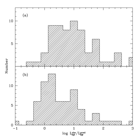
Figure 9: Histogram distribution of the ratio of the observed $L_{H\beta}$ to the values predicted by the stellar components in the base. (a): only one at 5 Myr; (b): 1, 3 and 5 Myr models.

To summarize, besides the presence of weak (scattered) broad-line components in some nuclei, our optical spectra do not provide us with reliable direct tracers of the properties, nor even of the existence, of the hidden AGN in the nuclear regions of nearby low-luminosity Seyfert 2 galaxies.

4.2 Starbursts versus Monsters

Within the ambiguities of the FC discussed above, the parameter $f_{AGN}=1-f_{SB}$ should provide us with at least a hint of the ionizing power of the elusive hidden AGN. Figure 10 plots the relation between $f_{AGN}$ and nebular excitation. In order not to crowd the plots we have left out the HeII lines for which we do not see any significant correlations, and which may be compromised by Wolf-Rayet features.

Figure 10: Relationships between the maximum Lyman ionization power produced by a hidden AGN component, $f_{AGN}$, and two indicators of the excitation of the nebular gas. As before, open squares correspond to objects with HBLRs.

While these plots show an intriguing structure, there is no obvious correlation between AGN fraction and excitation. Moreover, objects with putative HBLRs (open symbols) do not seem to stand out in these plots either. Since excitation is one of the classification criteria for Seyferts, these plots indicate that $f_{AGN}$ is not a very good starburst/monster discriminator. Another potentially powerful indicator of accretion power is hard X-ray luminosity. Figure 11 (left panel) shows the relation between $f_{AGN}$ and absorption-corrected hard X-ray luminosity. The lower-limits (arrows) correspond to Compton self-absorbed objects (hydrogen column densities $\rm>10^{24}cm^{-2}$) for which only reflected X-rays are observed. The right panel shows $L_{X}$ as a function of [OIII]/[OII].

Figure 11: Relationships between $f_{AGN}$, nebular excitation and hard X-ray luminosity. Arrows show Compton self-absorbed galaxies for which the X-ray luminosities are lower-limits. Galaxies with direct indications of a hidden BLRs are plotted as open squares.

There is no correlation between hard L_X and AGN fraction, but there is a clear trend of nebular excitation being higher for more X-ray luminous objects. These plots also show very clearly that nuclei with HBLRs have high X-ray luminosities, although the interpretation of this result is not straightforward since there may be a substantial contribution to the X-rays from off-nuclear sources (Jimenez-Bailón et al., 2003; Levenson et al., 2005). It is therefore relevant to examine the relation between X-ray luminosity and the global parameters of the sample: velocity dispersion and H$\beta$ luminosity. These relations are presented in Figure 12 where we see a weak trend of $L_{X}$ with $\sigma_{\rm[OIII]}$, but a significant correlation with L(H$\beta$) which is not a distance effect because it is also present in the fluxes. This is shown in Figure 13 where for clarity we have omitted the lower-limits. The line shows the OLS fit to the data of slope $1.1\pm 0.2$ ($R_{S}=0.19$) so, with large scatter, the X-ray power is roughly proportional to the Lyman ionizing power. Since we have no control over the spatial regions covered by the two data sets, we should be very careful about how to interpret this plot. Taken at face value it means that the bulk of the X-rays are produced by the same sources that photoionize the gas. This is consistent with the fact that the few objects with [OIII]/H$\beta<3$ (cf. Figure 10) lie below the best fitting line.

Figure 12: Correlations between (2-10keV) X-ray luminosity, nebular velocity dispersion ($\sigma_{\rm[OIII]}$), and H$\beta$ luminosity. As before, arrows correspond to Compton self-absorbed lower limits, and open symbols to galaxies with hidden BLRs.

Figure 13: 2-10keV X-ray flux against H$\beta$ flux. We have omitted the Compton self-absorbed sources for clarity. The line shows the best fitting line of slope unity.

Since even using deep high resolution X-ray (Chandra) and UV (HST) images it remains extremely difficult to see the AGN in nearby Seyfert 2’s ( e.g.. Jiménez-Bailón et al. 2003; Levenson et al. 2005), and since even when it is seen, there is still a significant contribution from circum-nuclear sources, the only way to answer the Starburst or Monsters question is to have deep high spatial resolution images of a substantial sample of nearby Seyfert 2 galaxies over a wide wavelength range. Until this is available, the interpretation of integrated observations will be plagued with the same uncertainties that we have confronted in the present work.

The INTEGRAL satellite has recently unveiled a putative new class of powerful, highly obscured, X-ray sources associated with massive stars: High Mass X-ray Binaries (HMXBs; Chaty and Filliatre, 2005). If HMXB’s represent a stage in the evolution of high-mass binaries, they could be very abundant in the circumnuclear starbursts presented in many Seyfert 2s, and thus potentially explain their X-ray morphologies.

5 Conclusions

We have presented a study of pure emission line spectra of a sample of 65 Seyfert 2 galaxies obtained by subtracting the synthetic stellar component from the observed spectra. Our main results are summarized as follows.

(i) For most Seyfert 2 galaxies, the gaseous nebular extinction deduced from the Balmer decrements appears to be systematically larger than the stellar extinction.

(ii) We compare the velocity dispersion of the stars and ionized gas, and confirm the existence of correlation between stellar and nebular velocity dispersion.

(iii) Seyfert 2 nuclei follow a Faber-Jackson like correlation between nuclear continuum luminosity and stellar velocity dispersion, but nuclei which also harbor star-formation deviate systematically from this relation. Removing the young stars from the continuum luminosity (using the synthesis results) strengthens the correlation substantially, and results in a slope more compatible with the actual Faber-Jackson relation.

(iv) There is a relation between ionized gas velocity dispersion and emission-line luminosities. We also find that Seyfert 2s with indication of broad lines either from the pure emission line spectrum or spectropolarimetric observations show larger [OIII] luminosities.

(v) We confirm our earlier inference that photoionization by young stars can explain a substantial fraction of the nuclear emission-line luminosities of Seyfert 2 nuclei, but neither the parameters derived from our optical spectra, nor the hard X-ray luminosities provide accurate indicators of the AGN contribution.

(vi) Albeit with substantial scatter, there is a correlation between hard (2-20keV) X-ray luminosity and H$\beta$ luminosity for our sample of low-luminosity AGN. The recent discovery of a new population of highly obscured luminous X-ray sources associated with high mass stars may yield some new clues to the interpretation of the properties of low-luminosity Seyfert galaxies. The off-nuclear X-ray sources detected by Chandra in some of these galaxies may, in the end, be powered by the same starbursts that are producing the bulk of the optical emission.

References

- [] Bassani L. et al. 1999, ApJS, 121, 473
- [] Bruzual G., Charlot S., 2003, MNRAS, 344, 1000
- [] Calzetti D., Kinney A., Storchi-Bergmann T., 1994, ApJ, 429, 582
- [] Cardelli J. A., Clayton G. C., Mathis J. S., 1989, ApJ, 345, 245
- [] Chaty, S., Filliatre, P., 2005, ApSS, 297, 235
- [] Cid Fernandes R., Heckman T., Schmitt H., González Delgado R.M., Storchi-Bergmann T., 2001, ApJ, 558, 81
- [] Cid Fernandes R., Gu Q., Melnick J., Terlevich E., Terlevich R., Kunth D., Rodrigues Lacerda R., Joguet B., 2004, MNRAS, 355, 273 (Paper II)
- [] Cid Fernandes R., Mateus A., Laerte S. Jr, Stasinska G., Gomes J. M., 2005, MNRAS, 358, 363
- [] Collinge M. J., Brandt W. N. 2000, MNRAS, 317, L35
- [] Croom S., Rhook K., Corbett E., et al. 2002, MNRAS, 337, 275
- [] Della Ceca R. et al., 2001, A&A, 375, 781
- [] Faber S. M., Jackson R. E. 1976, ApJ, 204, 668
- [] Garcia-Rissmann A., Vega L. R., Asari N. V., et al. 2005, MNRAS, 359, 765
- [] Gonzalez Delgado R.M., Heckman T., Leitherer C.,2001, ApJ, 546, 845.
- [] González Delgado R., Cerviño M., Martin L., Leitherer C., Hauschildt P.H., 2005, MNRAS, 357, 945
- [] Gu Q., Huang J., Ji L. 1998, ApSS, 260, 389
- [] Gu Q., Huang J., 2002, ApJ, 579, 205
- [] Hao L., Strauss M.A., Fan X., et al., 2005, AJ, 129, 1795
- [] Heckman T.M., Miley G.K., van Breugel W.J.M., Butcher H.R., 1981, ApJ, 247, 403
- [] Heckman T.M., González-Delgado R., Leitherer C., Meurer G.R., Krolik J., Wilson A.S., Koratkar A., Kinney A., 1997, ApJ, 482, 114
- [] Ho L. C.; Filippenko A. V.; Sargent W. L. W., 2003, ApJ, 583, 159
- [] Ho L. C. 2005, ApJ, 629, 680
- [] Isobe T., Feigelson E., Akritas M., Babu G., 1990, ApJ, 364, 104
- [] Iwasawa K., Maloney P. R., Fabian A. C. 2002, MNRAS, 336, L71
- [] Kauffmann G., Heckman T., White S., et al., 2003a, MNRAS, 341, 33
- [] Kauffmann G., Heckman T., Tremonti C., et al., 2003b, MNRAS, 346, 1055
- [] Jiménez-Benito L., Diaz A., Terlevich R., Terlevich E., 2000, MNRAS, 317, 907
- [] Jiménez-Bailón E., Santos-Lleó M., Mas-Hesse J.M., Guainazzi M., Colina L., Cerviño M., González Delgado R.M., 2003, ApJ, 593, 127
- [] Joguet B., 2001, PhD thesis, Inst. D’Astrophys. de Paris
- [] Joguet B., Kunth D., Melnick J., Terlevich R., Terlevich E., 2001, A&A, 380, 19. (Paper I)
- [] Levenson N.A., Weaver K.A., Heckman T.M., Awaki H., Terashima Y., 2005, ApJ, 618, 167
- [] Lumsden S. L., Alexander D. M., Hough J. H., 2004, MNRAS, 348, 1451
- [] Maiolino et al. 1998, A&A, 338, 781
- [] Mas-Hesse J.M., Kunth D., 1999, A&AS, 349, 765
- [] Matsumoto C., Nava A., Maddox L. A. et al. 2004, ApJ, 617, 930
- [] McCall M., Rybski P., Shields G., 1985, ApJS, 57, 1
- [] Mulchaey J. et al. 1994, ApJ, 436, 586
- [] Nelson C., Whittle M., 1995, ApJS, 99, 67
- [] Nelson C., Whittle M., 1996, ApJ, 465, 96
- [] Osterbrock D. E., 1989, Astrophysics of Gaseous Nebulae and Active Galactic Nuclei (Mill Valley: University Science Books)
- [] Osterbrock D. E., Shuder J. M., 1982, ApJS, 49, 149
- [] Peimbert M., Torres-Peimbert S., 1981, ApJ, 245, 845
- [] Polletta et al. 1996, ApJS, 106, 399
- [] Press W. H., Teukolsky S. A., Vetterling W. T., Flannery B. P., 1992, Numerical Recipes in Fortran, Cambridge University Press.
- [] Risaliti G., Gilli R., Maiolino R., Salvati M. et al. 2000, A&A, 357, 13
- [] Rosa M., 1985, Messenger, 39, 15
- [] Storchi-Bergmann T., Raimann D., Bica E.L.D., Fraquelli H. A., 2000, ApJ, 544, 747
- [] Terashima Y., Iyomoto N., Ho L., Ptak A. F. 2002, ApJS, 139 1
- [] Torres-Peimbert S., Peimbert M., Fierro J., 1989, ApJ, 345, 186
- [] Tremonti C., 2003, PhD thesis, John Hopkins University
- [] Whittle M., 1992a, ApJ, 387, 109
- [] Whittle M., 1992b, ApJ, 387, 121
- [] Whittle M., 1992c, ApJS, 79, 49
- [] Wilson A. S., Nath B., 1990, ApJS, 74, 731