Vertical Structure of Gas Pressure-Dominated Accretion Disks with Local Dissipation of Turbulence and Radiative Transport

Abstract

We calculate the vertical structure of a local patch of an accretion disk in which heating by dissipation of MRI-driven MHD turbulence is balanced by radiative cooling. Heating, radiative transport, and cooling are computed self-consistently with the structure by solving the equations of radiation MHD in the shearing-box approximation. Using a fully 3-d and energy-conserving code, we compute the structure of this disk segment over a span of more than five cooling times. After a brief relaxation period, a statistically steady-state develops. Measuring height above the midplane in units of the scale-height predicted by a Shakura-Sunyaev model, we find that the disk atmosphere stretches upward, with the photosphere rising to $\simeq 7H$, in contrast to the $\simeq 3H$ predicted by conventional analytic models. This more extended structure, as well as fluctuations in the height of the photosphere, may lead to departures from Planckian form in the emergent spectra. Dissipation is distributed across the region within $\simeq 3H$ of the midplane, but is very weak at greater altitudes. As a result, the temperature deep in the disk interior is less than that expected when all heat is generated in the midplane. With only occasional exceptions, the gas temperature stays very close to the radiation temperature, even above the photosphere. Because fluctuations in the dissipation are particularly strong away from the midplane, the emergent radiation flux can track dissipation fluctuations with a lag that is only 0.1–0.2 times the mean cooling time of the disk. Long timescale asymmetries in the dissipation distribution can also cause significant asymmetry in the flux emerging from the top and bottom surfaces of the disk. Radiative diffusion dominates Poynting flux in the vertical energy flow throughout the disk.

1 Context

If accretion disks radiate dissipated energy more quickly than their material moves inward, simple energy conservation determines their effective temperature as a function of radius $r$: it is

$$T_{\rm eff}=\left[\frac{3}{8\pi\sigma}\frac{GM\dot{M}R(r)}{r^{3}}\right]^{1/4},$$ (1)

where $\sigma$ is the Stefan-Boltzmann constant, the central mass is $M$, the accretion rate is $\dot{M}$, and $R(r)$ is a correction factor (close to unity at large radius) that accounts for the effect of the net angular momentum flux through the disk and relativistic corrections. Inside the disk, the temperature is often supposed to increase $\propto\tau^{1/4}$ (for optical depth from the surface $\tau$), in keeping with conventional local thermodynamic equilibrium (LTE) stellar atmosphere theory (e.g., as in Shakura & Sunyaev 1973). This guess about the internal temperature gradient is founded, however, upon the tacit assumption that the outgoing flux is created mostly near the midplane, which may or may not be true in real disks. Unfortunately, despite all the effort that has been expended upon accretion disk dynamics, there has been as yet only very limited attention given to their thermal structure (Brandenburg et al., 1995; Turner, 2004)

The true temperature profile matters in a number of ways. It is, of course, the fundamental parameter governing vertical hydrostatic balance, whether the pressure is dominated by gas or radiation. Thus, the disk’s thickness depends upon it. In addition, for known effective temperature (see equation 1), the spectrum emergent from any particular ring depends most strongly on the gravity at the photosphere. In thin disks, the vertical component of gravity increases linearly with height, so the temperature profile governs this quantity as well. Whether conventional plane-parallel, time-steady stellar atmosphere theory even applies to accretion disks also depends on whether the temperature (and density) structure is sufficiently homogeneous and stationary, one more open question.

Still another aspect of accretion disks for which knowledge of the vertical temperature profile is vital is the origin of hard X-ray emission. A very-nearly ubiquitous property of accretion disks around black holes, it appears on phenomenological grounds to find its origin in a “coronal” region somewhere near the disk surface. It is widely assumed that somehow the vertical temperature profile must accommodate a sharp upward rise above the photosphere, as the highest $T_{\rm eff}$ even in disks around relatively low-mass black holes ($\sim 10M_{\odot}$ is merely $\sim 10^{7}$ K, whereas the observed hard X-rays demand $T_{e}\sim 10^{9}$ K.

With the recognition that accretion is due to magnetohydrodynamic (MHD) turbulence driven by an underlying magneto-rotational instability (MRI: see, e.g., the review by Balbus & Hawley, 1998), the path toward answering these questions has been laid out, at least in principle: Track the dissipation that must occur at the short lengthscale end of the turbulent cascade; use known radiation physics to relate heat injection to photon production; compute photon transfer to the surface. The result of following this program will be a complete description of the disk equation of state and thermodynamics.

It is the object of this paper to report a step toward carrying out this project. As we will describe at greater length in the body of the paper, we have simulated a shearing-box section of a gas-dominated accretion disk in a manner that captures all numerically-dissipated energy. We suppose that this energy is transformed into local heating, and then solve the radiation transfer problem in the flux-limited diffusion (FLD) approximation. With this method, we are able to find the internal profiles of dissipation rate and temperature, as well as gas density and other interesting physical quantities. We are also able to study the character of fluctuations, both spatial and temporal.

Of all the many previous numerical studies of accretion disk properties that have been done to explore the consequences of MRI-driven MHD turbulence, the work by Miller & Stone (2000) is the one that most closely approached these questions before the present effort. In that paper, they explored the vertical structure of MHD turbulence within a shearing-box, but did so making a simplifying assumption about the gas thermodynamics: that the equation of state was isothermal. We will use their results as a standard of comparison in order to clarify which of our findings depend on explicit calculation of the gas’s thermodynamics, and which may be found on the basis of simpler arguments.

2 Calculation

The subject of our simulation is a radially thin slice of a gas-dominated accretion disk. We approximate the dynamics of this slice by a shearing box. That is, if we denote the radial coordinate by $x$, the azimuthal coordinate by $y$, and the vertical coordinate by $z$, we assume there are underlying (unsimulated) dynamics that produce an azimuthal velocity $v_{y}=-(3/2)\Omega x$, where $\Omega$ is the orbital frequency and the zero-point of $x$ is in the center of the box. Because this shearing-box is meant to approximate a section of an orbiting disk, we also assume a Coriolis force and appropriate gravitational tidal forces.

2.1 Basic Equations and their Solution

The equations we solve to describe the dynamics of this box are the frequency-averaged equations of radiation MHD in the FLD approximation:

$$\frac{\partial\rho}{\partial t}+\nabla\cdot\left(\rho\mbox{\boldmath$v$}\right)=0$$ (2)

$$\frac{\partial\rho\mbox{\boldmath$v$}}{\partial t}+\nabla\cdot\left(\rho\mbox{\boldmath$v$}\mbox{\boldmath$v$}\right)=-\nabla(p+q)+\mbox{\boldmath$j$}\times\mbox{\boldmath$B$}+\frac{\chi\rho}{c}\mbox{\boldmath$F$}$$

$$\qquad-2\rho\left(\Omega\hat{\mbox{\boldmath$z$}}\right)\times\mbox{\boldmath$v$}+3\rho\Omega^{2}x\hat{\mbox{\boldmath$x$}}-\rho\Omega^{2}z\hat{\mbox{\boldmath$z$}}$$ (3)

$$\frac{\partial E}{\partial t}+\nabla\cdot\left(E\mbox{\boldmath$v$}\right)=(4\pi B-cE)\kappa\rho-\nabla\mbox{\boldmath$v$}:\mathsf{P}-\nabla\cdot\mbox{\boldmath$F$}$$ (4)

$$\frac{\partial e}{\partial t}+\nabla\cdot\left(e\mbox{\boldmath$v$}\right)=-(4\pi B-cE)\kappa\rho-\left(\nabla\cdot\mbox{\boldmath$v$}\right)(p+q)+Q$$ (5)

$$\frac{\partial\mbox{\boldmath$B$}}{\partial t}+\nabla\times\mbox{\boldmath$E$}=0$$ (6)

$$\mbox{\boldmath$F$}=-\frac{c\Lambda}{\chi\rho}\nabla E$$ (7)

The quantities $\rho$, $e$, and $v$ are the density, internal energy, and velocity field of the gas. The pressure of the gas $p$ is related to the internal energy by $p=(\gamma-1)e$ with the adiabatic index $\gamma$ (here $\gamma=5/3$ is assumed). $q$ is the stress associated with a small artificial bulk viscosity employed, in the usual manner, to suppress post-shock ringing by capturing the shock’s entropy generation. $Q$ represents the rate at which the internal energy must be changed in order for total energy to be conserved (see Appendix A). $B$ is the magnetic field, $\mbox{\boldmath$j$}=\nabla\times\mbox{\boldmath$B$}/(4\pi)$ is the current density, and $\mbox{\boldmath$E$}=-\mbox{\boldmath$v$}\times\mbox{\boldmath$B$}$ is the electric field.

The radiation field is described by the energy density $E$, flux $F$, and pressure tensor $\mathsf{P}$. The equations are closed with the relation $\mathsf{P}=\mathsf{f}E$, where $\mathsf{f}$ is the Eddington tensor, which is defined in terms of the scalar Eddington factor $f$:

$$\mathsf{f}=(1/2)(1-f)\mathsf{I}+(1/2)(3f-1)\mbox{\boldmath$\hat{n}$}\mbox{\boldmath$\hat{n}$}.$$ (8)

The Eddington factor is in turn assumed to depend on the flux limiter $\lambda$ and the dimensionless opacity parameter $R\equiv|\nabla E|/(\chi\rho E)$ through the relation,

$$f=\lambda+\lambda^{2}R^{2}$$ (9)

(Turner & Stone, 2001), where $\lambda=(2+R)/(6+3R+R^{2})$ (Levermore & Pomraning, 1981). Assuming LTE, the radiation emission rate is simply the Planck function, $B$. Appropriately averaging the frequency-dependent free-free opacity, the Planck-mean opacity $\kappa$ depends on the other parameters as $3.7\times 10^{53}\sqrt{\rho^{9}/e^{7}}$ cm² g^-1 (one of the reasons we choose a comparatively small central mass, $6.62M_{\odot}$, for this simulation is to reduce the contribution of other mechanisms to the absorptive opacity). Both free-free absorption and Thomson scattering are included in the Rosseland-mean opacity $\chi$ ($=1.0\times 10^{52}\sqrt{\rho^{9}/e^{7}}+0.33$ cm² g^-1).

For the problem studied in this paper, the thermodynamics and vertical structure of a gas pressure-dominated disk, the radiation force term in equation 3 might seem superfluous. We retain it for two reasons. First, although in the conditions treated here the radiation force is relatively small, it still contributes at the tens of percent level. Second, one of our long-term goals in this effort is to study disks in which radiation forces are more important, so we wish to develop techniques capable of describing them.

It is also worth commenting that there are some problems in which the gas’s radiative losses could be treated more simply. If, for example, the ion temperature is elevated far above the electron temperature (Ichimaru, 1977; Rees et al., 1982; Narayan & Yi, 1994), the density in the disk can be so low that the optically thin limit can apply.

The tool we use to solve these equations is the latest version of the radiation/MHD code first described in Stone & Norman (1992a, b), and then successively modified by Turner & Stone (2001), Turner et al. (2003) and again by Turner (2004). We have further improved it. The most important change in terms of its applicability to this scientific problem is that it now conserves energy quite accurately by means of a special internal energy update scheme designed to ensure that all numerical losses of kinetic and magnetic energy are captured in the form of heat added to the gas internal energy (details in Appendix A). In this way, these equations mimic the much more complex physics of magnetic reconnection and other kinetic processes.

In addition, we have also made several technical improvements. Two are worth noting here. First, instead of the Alternating Direction Implicit (ADI) method used by Turner & Stone (2001) to solve the radiation diffusion equation, we now employ the Gauss-Seidel method accelerated by a full multi-grid method. When the ADI method was used with a shearing box boundary condition, maintaining stability restricted the time step $\Delta t$ to be shorter than the diffusion time step. Our code is free from this restriction because the Gauss-Seidel method solves the diffusion equation in a directionally unsplit way. The Courant number for the radiation diffusion can be as large as $\sim 10^{2}$ in our simulation.

Second, in every grid-based hydrodynamics simulation with explicit time-advance, the Courant condition puts an upper limit on the time-step that can be used. In this case, we evaluate this limit in terms of the time for an acoustic wave supported by gas, magnetic, and radiation pressure to cross a grid-zone. This time is much shorter in the low-density regions above the photosphere than in the midplane because the ratio of radiation pressure to density is very large there. Consequently, the time-step is governed primarily by the lowest-density zones. If the density there were permitted to be as small as the dynamics demanded, a prohibitive number of time-steps would be required in order to complete the simulation. In the closely-related work of Turner (2004), a lower bound of $2\times 10^{-3}$ of the maximum density in the initial state was placed on the density in order to prevent such a computational slow-down. However, invocation of the density floor effectively means injection of energy into the problem because the newly-created mass is given the local velocity and implicitly acquires the local potential energy. To enhance the quality of our energy conservation while still limiting the total computing time required to a reasonable amount, we set this floor at $10^{-5}$ of the midplane density. At this value, the total amount of energy injected due to the density floor is $\simeq 0.9\%$ of the total heat dissipation over the 60 orbits of the simulation. Further details about this procedure (and the smaller effects of some other variable caps) may be found in Appendix A.3.

2.2 Parameters

The physical conditions in such a slice are determined by three parameters: the central black hole mass $M$, the central radius of the slice $r$, and the surface density $\Sigma$. The values we have chosen for them are meant to be representative of conditions in an accretion disk around a Galactic black-hole binary relatively far from the black hole itself: $M=6.62M_{\odot}$, $r=300r_{g}$, and the surface density predicted by an $\alpha=0.03$ Shakura-Sunyaev disk model with an accretion rate $\dot{M}$ that would yield a total luminosity of $0.1L_{E}$ if the radiative efficiency in rest-mass units were 0.1. The effective temperature at the surface of such a disk segment is $5.3\times 10^{5}$ K. These parameters can be combined to define a characteristic scale-height $H$ after estimating the temperature rise toward the center of the disk. In such a model, the relation between surface density and accretion rate is

$$\Sigma_{0}=\left(\frac{\pi\sigma}{3\chi}\right)^{1/5}\left(\frac{\mu}{\pi\alpha k}\right)^{4/5}\dot{M}^{3/5}\Omega^{2/5}R^{3/5}(r).$$ (10)

The symbols $\mu$, $k$, and $\sigma$ in this expression are the mean mass per particle, the Boltzmann constant, and the Stefan-Boltzmann constant, respectively. Numerical values for these and a number of other parameters of interest are collected in Table 1 (note that in the shearing-box approximation, $R(r)\equiv 1$).

Table 1: Simulation Parameters

Parameter	Definition	Value	Comment
$M$	$6.62M_{\odot}$	$1.31\times 10^{34}$ g	mass of central black hole
$\dot{M}$	$0.1(L_{E}/c^{2})/\eta$	$7.52\times 10^{17}$ g s-1	estimated mass accretion rate
$\alpha$		$0.03$	estimated stress/pressure ratio
$r$	$300(GM/c^{2})$	$2.93\times 10^{8}$ cm	radius
$\Omega$	$\sqrt{GM/r^{3}}$	$5.90$ s-1	orbital frequency
$T_{\rm orb}$	$2\pi/\Omega$	$1.06$ s	orbital period
$H$	$c_{\rm g}/\Omega$	$3.53\times 10^{6}$ cm	disk scale-height
$F_{0}$	$(3\dot{M}\Omega^{2})/8\pi$	$3.12\times 10^{18}$ erg cm-2 s-1	estimated radiation flux at surface
$\Sigma_{0}$	eq.[10]	$9.89\times 10^{4}$ g cm-2	surface density
$\rho_{0}$	$\Sigma_{0}/(2H)$	$1.40\times 10^{-2}$ g cm-3	mean density

2.3 Initial Conditions

Our initial condition is (almost) the Shakura-Sunyaev equilibrium corresponding to our chosen parameters. In this equilibrium, the gas and the radiation are assumed to be in a planar hydrostatic and thermal equilibrium state everywhere below the photosphere. Our initial condition differs from the Shakura-Sunyaev assumptions in taking the local dissipation rate proportional to the logarithm of the column density to the surface, a dissipation profile adopted on the basis of some previous numerical experiments. Under these assumptions, the basic equations (3), (4)+(5), and (7) are reduced to

$$-\frac{dp}{dz}+\frac{\chi\rho}{c}F-\rho\Omega^{2}z=0$$ (11)

$$\frac{dF}{dz}=-\frac{F_{0}}{\ln\tau_{0}}\frac{d\ln\Sigma}{dz}$$ (12)

$$F=-\frac{c}{3\chi\rho}\frac{dE}{dz},$$ (13)

where $\tau_{0}\equiv\int_{0}^{z_{\rm surface}}\chi\rho dz=\chi\Sigma_{0}/2$ is the total optical depth and we assume the opacity is entirely Thomson scattering. The boundary condition on this set of equations is that the radiative flux at the photosphere ($\tau=1$) of the disk must match the total dissipation rate (eq.[1]), or $F_{0}$. Lastly, the gas is also assumed to be in thermal equilibrium with the radiation ($E=aT^{4}$).

Outside the photosphere, the flux is constant ($F=F_{0}$), the gas density is set to the density floor (see § 2.1), and its temperature is constant at the effective temperature, $4.8\times 10^{5}$ K. Because its total pressure is then very nearly constant with height, this gas has almost no support against gravity.

The shapes of the initial gas density and pressure profiles are displayed in Figures 1 and 2. As expected, the ratio of radiation pressure to gas pressure in the midplane is small, $0.039$ in the initial state, placing this equilibrium well within the gas-dominated regime. With such a large surface density, the disk is also very optically thick: its (half)-Thomson depth is $\tau_{0}=1.63\times 10^{4}$. Although the absorptive opacity is never more than $\simeq 6\%$ of the Rosseland mean, the effective optical depth to the midplane is also so large ($\int_{0}^{z_{\rm surface}}\sqrt{\kappa\chi}\rho dz=4.04\times 10^{3}$) that we expect the radiation to be well-coupled thermally to the gas except on very short lengthscales and at very high altitude. This expectation is strongly vindicated in the simulation (Fig. 3).

The initial configuration of the magnetic field is a twisted azimuthal flux tube of circular cross section with radius $0.75H$ whose center is placed at $x=z=0$. The field strength in the tube is uniform at $2.16\times 10^{6}$ G, and its maximum poloidal part is $5.40\times 10^{5}$ G, corresponding to an initial plasma $\beta\equiv p/(\mbox{\boldmath$B$}^{2}/8\pi)=24$. The corresponding maximum MRI wavelength in the midplane is $\lambda_{\rm max}\equiv(8\pi/\sqrt{15})(v_{A}/\Omega)=1.59\times 10^{6}$ cm, which is resolved with $7.2$ grid zones (Balbus & Hawley, 1998).

The calculation is begun with a small random perturbation in the poloidal velocity. The maximum amplitude of each velocity component is $1$% of the local magnetosonic speed $c_{s}$, in which we include radiation in the total pressure.

2.4 Grid and Boundary Conditions

The computational domain extends $2H$ along the radial direction, $8H$ along the orbit, and $8H$ on either side of the midplane. It is divided into $32\times 64\times 256$ cells ($x\times y\times z$) with constant grid size $\Delta x=\Delta z=H/16=\Delta y/2$. The grid is staggered, with scalar quantities ($e$, $E$, and $\rho$) defined at zone-centers and vector quantities ($v$, $B$, and $F$) defined on zone-surfaces.

The azimuthal boundaries are periodic and the radial boundaries are shearing-periodic in the local shearing-box approximation (Hawley, Gammie, & Balbus, 1995). We desire the vertical boundaries to be outflow (free) boundaries; that is, we endeavor to determine the values in the ghost cells so that mass, momentum and energy fluxes across the boundaries are the same as those across the adjacent cell surfaces. However, the vertical disk structure is approximately hydrostatic, so motions across the top and bottom boundaries are in general subsonic. Imperfections in the boundary conditions can therefore act as noise sources for perturbations able to travel into the problem area. We found in practise that many natural realizations of outflow boundary conditions for this problem suppressed noise-generation sufficiently well that little was seen for tens of orbits, but dramatically elevated values of one or more of the code variables would then suddenly appear in a small number of cells and disrupt the simulation. The particular version of outflow boundary conditions we present in the next few paragraphs was able to suppress such artifacts for the entire 60 orbit span of this simulation.

For solving advection equations (steps 4 to 7 in Appendix A), the usual approach—a constant (zero slope) projection of variables into the ghost cells—works well. For solving the radiation diffusion equation (step 3 in Appendix A), it is better to set $E$ in the ghost cells so that the diffusion flux $F_{z}=-c\Lambda/(\chi\rho)dE/dz$ is constant (details are described in Appendix B). We tried both time-explicit and time-implicit versions of this method and found that (somewhat surprisingly) the explicit version was less likely to cause problems.

To prevent energy inflows, we adopt two additional conditions: (a) the $z$-component of the velocity at the boundary surface is set to zero when it is negative (positive) at the top (bottom) boundary (see Appendix A.3). (b) the radiation energy in the ghost cell is set equal to that in the adjacent cell when the former becomes larger than the latter.

For the magnetic field, we build upon the usual scheme in which the electric field is extrapolated into the ghost cells and the induction equation (eqn. 6) is solved in those cells to find the magnetic field. This approach ensures that $\nabla\cdot\mbox{\boldmath$B$}=0$ even in the ghost cells (the CT algorithm ensures it is zero in the entire problem area). It does not, however, guarantee that the magnetic field varies smoothly across the boundaries. To forestall jumps in the magnetic field intensity across the boundary, we introduce a small but finite resistivity into the ghost cells. This device also prevents the development of field-strength discontinuities at the boundary large enough to cause code crashes. After some experimentation, we found that these goals could be achieved with a ghost-cell resistivity set to $0.13\times{\min({\Delta x}^{2},{\Delta y}^{2},{\Delta z}^{2})}/\Delta t$. Note that our electric field extrapolation does not restrict the sign of the Poynting flux across the boundary (see section 3.2.1).

3 Results

The simulation ran for 60 orbits. Transients persisted for 5–10 orbits, and thereafter most properties maintained a statistically steady state. For example, during the period from 10 to 60 orbits, the outgoing flux varied within a total range of a factor of two, with an rms fractional variation of only 14%. We therefore regard the structure as having achieved a well-defined steady-state, and we begin by describing its time-average properties. In the following, the time average is done for 50 orbits, from $t=10$ orbits to $t=60$ orbits.

3.1 Mean Vertical Profiles

Our initial condition is (almost) a conventional model for a gas pressure-dominated disk: a (nearly-) Gaussian profile of gas density with characteristic scale $H$. However, the time-averaged density profile is considerably shallower in slope (Fig. 1). From a height $|z|\simeq 2H$ out to $\simeq 8H$, it is better described by an exponential with a slowly changing length-scale: the density scale-height is $\simeq 0.3H$ for $H\lesssim z\lesssim 5H$ and stretches to $\simeq 0.4H$ at greater altitude. This result echoes what was found by Miller & Stone (2000), but is different in detail: we find a broader region of slowly-declining density near the midplane (presumably do to our higher temperature there) and slightly steeper exponential decline outside that region.

Because the density falls relatively gradually with height, the mean altitude of the photosphere (defined as the point where the Eddington factor $f=0.5$: see § 3.2.3 for a more detailed discussion) is almost at the top of the box, $|z|\simeq 7.3H$. Thus, although most of the mass is contained within $\pm 2H$ of the midplane, in other respects the disk should be thought of as considerably thicker.

Clearly, something other than thermal gas pressure must support this extended atmosphere. What that is is revealed in Figure 2, where we display the profiles of gas pressure ($p=2e/3$), magnetic pressure ($p_{\rm mag}\equiv\mbox{\boldmath$B$}^{2}/8\pi$), and radiation pressure ($p_{\rm rad}\equiv E/3$), as well as the contribution of each of them to support against gravity. Although both the radiation pressure and the magnetic pressure are small compared to the gas pressure throughout the initial condition, both become greater than the gas pressure above $\simeq 3H$ in the equilibrium, with the magnetic pressure generally a few times greater than the radiation pressure. Deep inside the disk, hydrostatic support is mostly due to gas pressure. Although at higher altitudes the radiation pressure is comparable to the magnetic pressure, and both are larger than the gas pressure, the dominant vertical force is magnetic. The reason is that near the photosphere, where the radiation pressure is relatively large, its gradient is small. Thus, we find that the disk possesses an extended sub-photospheric magnetically-dominated atmosphere whose thickness is more than twice that of the gas pressure-supported disk body.

Although the magnetic field dominates at higher altitudes, the radiation pressure grows to exceed the magnetic field energy density near the midplane. From its initial midplane ratio of $\simeq 0.04$, $p_{\rm rad}/p$ grows to $\simeq 0.2$ in the steady state, about a factor of 6 greater than $p_{\rm mag}/p$ at that location. Similarly, the plasma $\beta$ (which was 24 in the midplane initially) grows to $\simeq 40$ there, but declines steeply with height, reaching a low of about 0.03 at $|z|\simeq 7H$. If the pressure used in the plasma $\beta$ is redefined as the sum of radiation plus gas pressure, the minimum $\beta$ is $\simeq 0.15$. These values are very similar to those previously found by Miller & Stone (2000), a midplane $\beta\simeq 40$ and $\beta(7H)\simeq 0.01$.

The gas temperature declines from a peak of about $4.5\times 10^{6}$ K at the midplane to a minimum $\simeq 7\times 10^{5}$ K, achieved in the range $5H\lesssim|z|\lesssim 7H$ (Fig. 3). Within $\simeq 5H$ of the midplane, LTE is an excellent approximation, as the gas and radiation temperatures are very close. In the outer most of that zone, the $\tau^{1/4}T_{\rm eff}$ approximation is fairly close to the actual temperature, but it overestimates the temperature by $\simeq 20\%$ within $\simeq H$ of the midplane. This overestimate is due to the finite vertical spread in the dissipation distribution (see section 3.2.2). At large $|z|$, the radiation temperature approaches the effective temperature (as it must). The time-averaged effective temperature is $\simeq 5.3\times 10^{5}$ K, about 10% higher than the temperature predicted by the Shakura-Sunyaev model. However, the gas temperature between $\simeq 5H$ and $7H$ exceeds the radiation temperature by about 30%.

Above $\simeq 7H$, the gas temperature rises toward our outer boundary. It is hard for us to determine how much of that rise is physical, and how much is due to the guesses required to impose an outer boundary on the magnetic field. We are led to suspect that much of it is a numerical artifact because roughness in the magnetic field near the boundary creates a spike in the time-averaged vertical profile of the dissipation density per unit mass, likely leading to this abrupt rise in temperature. However, as Figure 3 also shows, the radiation temperature decouples from the gas temperature near the gas temperature minimum, so that the outgoing radiation flux is hardly affected by the gas temperature spike near the boundary.

Lastly, we turn to the time-averaged stress. Even after both horizontal- and time-averaging, the stress profile still shows small-scale fluctuations and a distinct asymmetry—the peak is at $z\simeq 2H$, and is about 50% higher than the level at $z\simeq-2H$ (Fig. 5). In fact, we find that at any given time the magnetic field intensity and stress tend to be asymmetric about the midplane, with both a few times greater in one half than in the other. These asymmetries last for periods $\sim 10$ orbits before flipping to the other direction.

Like many other quantities, there is also a sharp contrast between the stress in the disk body region ($|z|\lesssim 3H$) and in the corona. Within the disk body region, the stress distribution is roughly independent of $z$, but outside that region, it declines sharply. Virtually all the stress is created in the disk body, with only about 10% above $|z|=3H$ and just 1% more than $5H$ from the plane. This pattern is qualitatively similar to the results of Miller & Stone (2000), who also found an approximately flat-topped stress distribution that extended a few scale-heights from the midplane; the only contrast is that in their work the drop toward the outside was not as steep.

Averaged over the length of the simulation, the total stress in the problem area was large enough to drive an accretion rate of $1.1\times 10^{18}$ g s^-1, 44% greater than our initially estimated accretion rate. This is why $T_{\rm eff}$ is 10% higher than as predicted by the Shakura-Sunyaev model, of course. Phrased in terms of the traditional $\alpha$ measure (ratio of vertically-integrated stress to vertically-integrated total pressure), we find $\alpha\simeq 0.02$ (note that the time-averaged vertically-integrated pressure is greater than in the initial condition). In evaluating this finding, it should be borne in mind that global disk simulations Hawley & Krolik (2001) generally find rather larger mean $\alpha$ measures than shearing-box simulations like this one. In addition, we find that this stress is very non-uniformly distributed. Measuring it in pressure units, it rises from $\simeq 0.01$ in the midplane to $\simeq 1$ at $|z|>6H$.

3.2 Thermal balance

3.2.1 Net energy flow

The history of energy flows into and out of the shearing box is displayed in Figure 4. The only physical source of energy for the problem volume is the work done on the inner and outer radial surfaces by magnetic and Reynolds stresses (about 77% magnetic), but there is also a small non-physical injection of energy whenever the density floor, energy floor, and/or velocity cap is invoked (see Appendix A.3). Energy loss in the simulation is entirely physical, and may occur through any of three channels: radiation, matter, and Poynting flux. Of these, radiation diffusion flux completely dominates the others: the time-averaged fraction in each flux at the outer boundaries is 99.71% (radiation–diffusion), 0.14% (radiation–advection), 0.25% (matter), -0.10% (Poynting flux: it can be negative because we do not prohibit it in the boundary conditions; see section 2.4.) Given the complete dominance of radiation as the energy output channel, it should not be surprising that its history tracks very closely the history of work done on the box. The flux cannot precisely follow the work, however, because it takes a finite time ($\sim 1$ orbit) for work to be transformed into heat and because it takes more time (in this case up to $\sim 10$ orbits) for the photons to diffuse out. The “lightcurve” is therefore a delayed and smoothed version of the work (see the following subsection).

Although the vertical radiation flux is always much larger than either the Poynting flux or the energy flux carried by gas motions, the ratios between the fluxes of these three channels change systematically with height (Fig. 6). In the inner half of the disk (i.e., $|z|\lesssim 3H$–$5H$), Poynting flux is present at an interesting but low level—$\simeq 5$–8% of the radiation flux; at greater height, the Poynting flux becomes much weaker. By the time the edge is reached, the Poynting flux is so small that numerical uncertainties in the boundary conditions lead to its time-average turning weakly negative, that is, in net it brings energy into the box. Matter outflow never contributes significantly. There is also a striking asymmetry in the magnitude of the flux between the two sides of the disk; this will be discussed further in § 3.3.4.

These results stand in some contrast to the earlier work on stratified disks by Miller & Stone (2000), where the Poynting flux through the $|z|=2H$ surface in their fiducial (toroidal field) simulation was several times greater, about 25% of the rate at which stresses did work on the walls of the box. In that simulation there were also “implicit radiation losses” associated with their isothermal equation of state.

That the Poynting flux should always be rather smaller than the total dissipation rate follows from the character of hydrostatic equilibrium in disks. The Poynting flux may be thought of as arising from magnetic buoyancy, and so can be expected to have a magnitude $\sim fc_{s}|\mbox{\boldmath$B$}|^{2}/8\pi$, where the factor $f$ represents the departure from hydrostatic balance that permits the upward motion. On the other hand, the total dissipation rate is $\sim(3/2)\phi(z)\Omega sH\langle B_{r}B_{\phi}\rangle_{0}/4\pi$, where $\phi$ is a profile function that rises from zero in the midplane to unity once all the dissipation has been accomplished, at $\simeq sH$ (as shown in the following subsection, $s\simeq 3$ here). The subscript $0$ labels the mean stress in the central body of the disk. Thus, the Poynting flux fraction is

$$\sim\frac{\sqrt{2}}{3}{f\over\phi s}{|\mbox{\boldmath$B$}|^{2}(z)\over\langle B_{r}B_{\phi}\rangle_{0}}$$

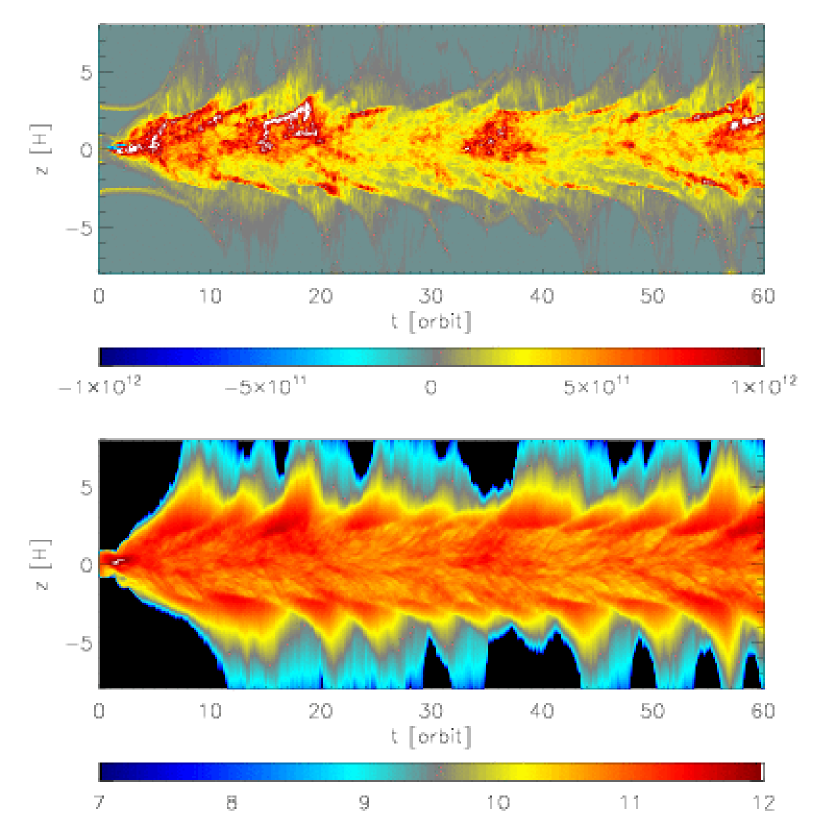
Figure 14: Top panel: Horizontally-averaged dissipation rate as a function of $z$ and $t$. Bottom panel: Horizontally-averaged magnetic field intensity.

because the scale-height $H\equiv c_{s}/(\sqrt{2}\Omega)$. In the central disk, the ratio of the magnetic field intensity to the stress is typically a few, making the Poynting flux fraction somewhat less than $\sim f$; at larger altitude, the ratio of the local magnetic field energy density to the stress in the central disk drops, and the Poynting flux becomes progressively less important. Thus, the maximum Poynting contribution is $\lesssim f$. In this simulation, we find that the mean rise speed of magnetic structures (as seen, e.g., in Fig. 14) is $\sim 0.1c_{s}$, indicating a maximum Poynting contribution $\sim 10\%$. It is possible that in other, less settled, circumstances $f$, and therefore the Poynting flux contribution, might be greater.

3.2.2 Dissipation rate

The energy brought into the problem volume by stresses on the radial surfaces is transformed into magnetic field energy and the kinetic energy of random fluid motions. As the turbulent cascade transfers this energy to smaller and smaller scales, eventually it is dissipated. A small part of this dissipation is associated with weak shocks (mostly at high altitude), but the great majority occurs on the grid-scale and is captured by our local energy conservation scheme, where it is transferred to gas internal energy. Because the step in our energy conservation scheme that captures magnetic energy dissipation also includes kinetic energy, we cannot fully separate which contributes how much to the total. What we can say is that in rough terms, 70% of the dissipation comes from the step that mixes the two, 20% is clearly associated with the loss of fluid kinetic energy, and 10% comes from our use of an artificial bulk viscosity. As we will shortly demonstrate, however, there is a strong correlation between dissipation rate and current density; this correlation suggests that much of the mixed-source 70% is due to magnetic energy. Two global measures of this dissipation are shown in Figures 5 and 7, its time- and horizontally-averaged vertical profile and its time-history.

The total dissipation rate varies by factors of several over time, but in the mean must result in an effective temperature at the surface as given by equation (1). As can be seen in the figure, its fluctuations follow very closely upon fluctuations in the total stress. Cross-correlating the two curves demonstrates that there is generally a lag of less than an orbit between stress and dissipation; that is, it takes no more than an orbit or so for energy injected by shear stresses at the boundary to traverse the turbulent cascade all the way to dissipation.

The mean vertical profile of the dissipation rate is, in rough terms, a “top-hat” stretching from $-3H$ to $+3H$. It is not coincidental that the dissipation rate drops sharply at the same place where magnetic pressure begins to exceed gas pressure. Dissipation is associated with sharp gradients, particularly in the magnetic field, driven by turbulence. At higher altitudes, the comparative strength of the field keeps its structure smooth and irons out sharp changes. For many of the same reasons, the vertical profile of the stress is very similar to that of the dissipation.

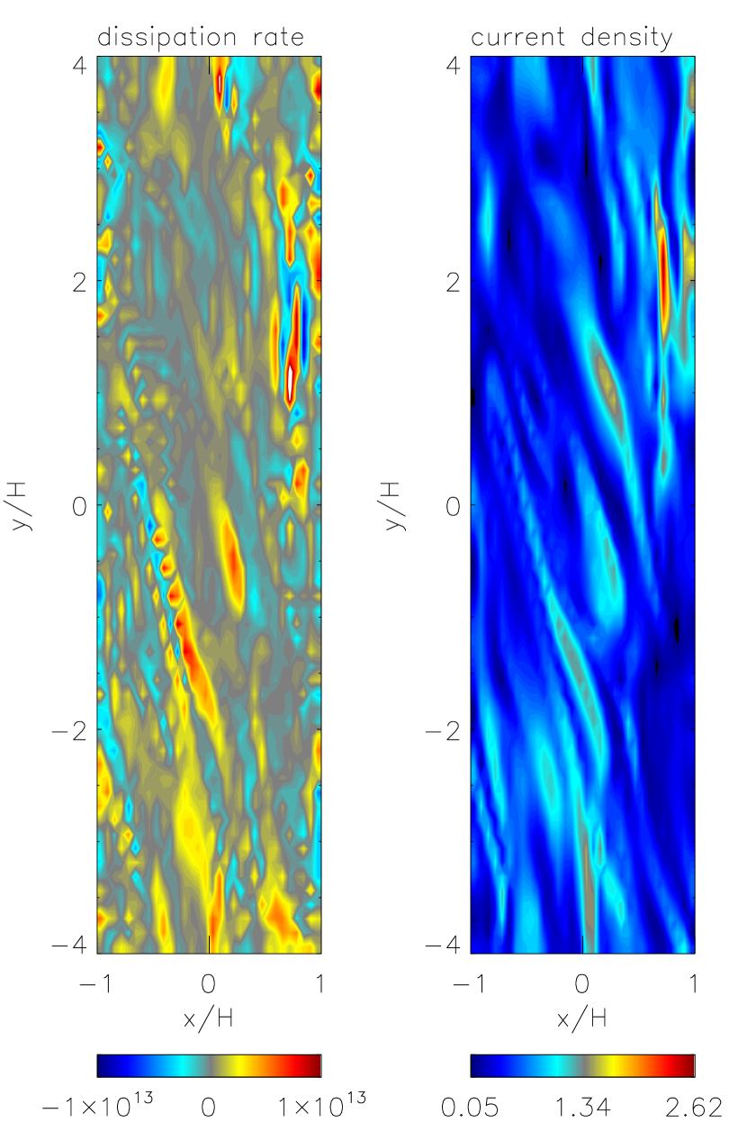
Figure 8: A horizontal slice at $z=0$ at $t=35$ orbits. Left panel: total dissipation rate (erg cm^-3 orbit^-1). Right panel: current density (esu cm^-2 s^-1).

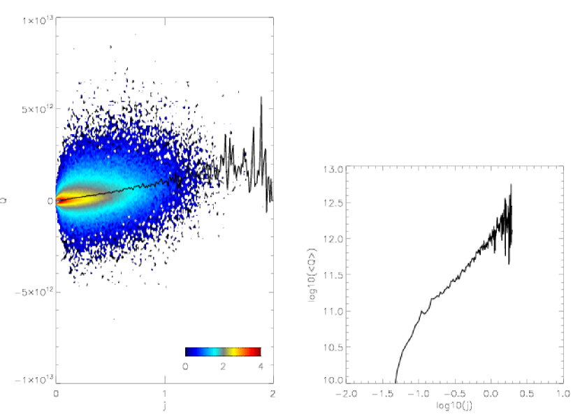
Figure 9: The relation between current density and dissipation. In the main panel, the color indicates (on a logarithmic scale) the number of cells having a given level of current density and dissipation rate at time $t=40$ orbits. The curve running through it (reproduced in the inset) shows $\langle Q\rangle$, the centroid of the dissipation distribution at fixed current density.

A different view of the distribution of dissipation is also instructive (Fig. 8). Although low-level dissipation can occur throughout the fluid due to numerical error, strong dissipation tends to be correlated with intense current, i.e., regions of large $|\nabla\mbox{\boldmath$B$}|$. A more quantitative view of the association between current density and dissipation can be seen in Figure 9, where we plot the number of cells $N$ having a given dissipation rate $Q$ and current density $|\mbox{\boldmath$J$}|$ at time $t=40$ orbits. At small values of the current density, a significant part of the local dissipation rate is due to random numerical errors. However, even when $|\mbox{\boldmath$J$}|$ is relatively small, there is always a bias to positive dissipation. Defining the centroid of the distribution by $\langle Q\rangle=\int\,dQ\,QN(Q,|\mbox{\boldmath$J$}|)/\int\,dQ\,N(Q,|\mbox{\boldmath$J$}|)$, we see that for the upper factor of 30 in its dynamic range, $\langle Q\rangle$ is well-described by a power-law $\propto|\mbox{\boldmath$J$}|^{1.13}$.

3.2.3 Cooling

The rate at which the heat content of the box equilibrates can be parameterized by the cooling time. In any accretion flow that radiates efficiently, conservation of angular momentum and energy require that $t_{\rm cool}\sim\alpha^{-1}P_{\rm orb}$. One way to evaluate it more quantitatively from the simulation data is to compute the ratio of the total energy content of the box to the energy flux leaving through its top and bottom surfaces. Using this approach, we find a cooling time of 11.4 orbits. In these terms, our simulation ran for a bit more than 5 cooling times, with 4 of them well after the erasure of initial transients.

However, another way to examine the delay between the creation of heat and its loss is to study the cross-correlation between the volume-integrated dissipation and the flux out of the box. That relationship is displayed in Figure 10. As this figure shows, fluctuations in the flux tend to follow those in the dissipation rate, but not by very much—although there is an asymmetric tail toward positive lags, the cross-correlation falls to zero by +10 orbits, and its peak occurs in the range 0–2 orbits. The reason that the cooling rate tracks the dissipation rate with a lag almost an order of magnitude shorter than the nominal cooling time is that the variance in the dissipation rate is dominated by the region $2H\leq|z|\leq 3H$, where the cooling time is 10 to 30 times shorter than from the midplane. Much of the dissipation fluctuation power is on timescales $\sim t_{\rm cool}$, but because the fluctuations take place in a region of quick cooling, there is nonetheless little time-lag in imprinting them on the radiation flux.

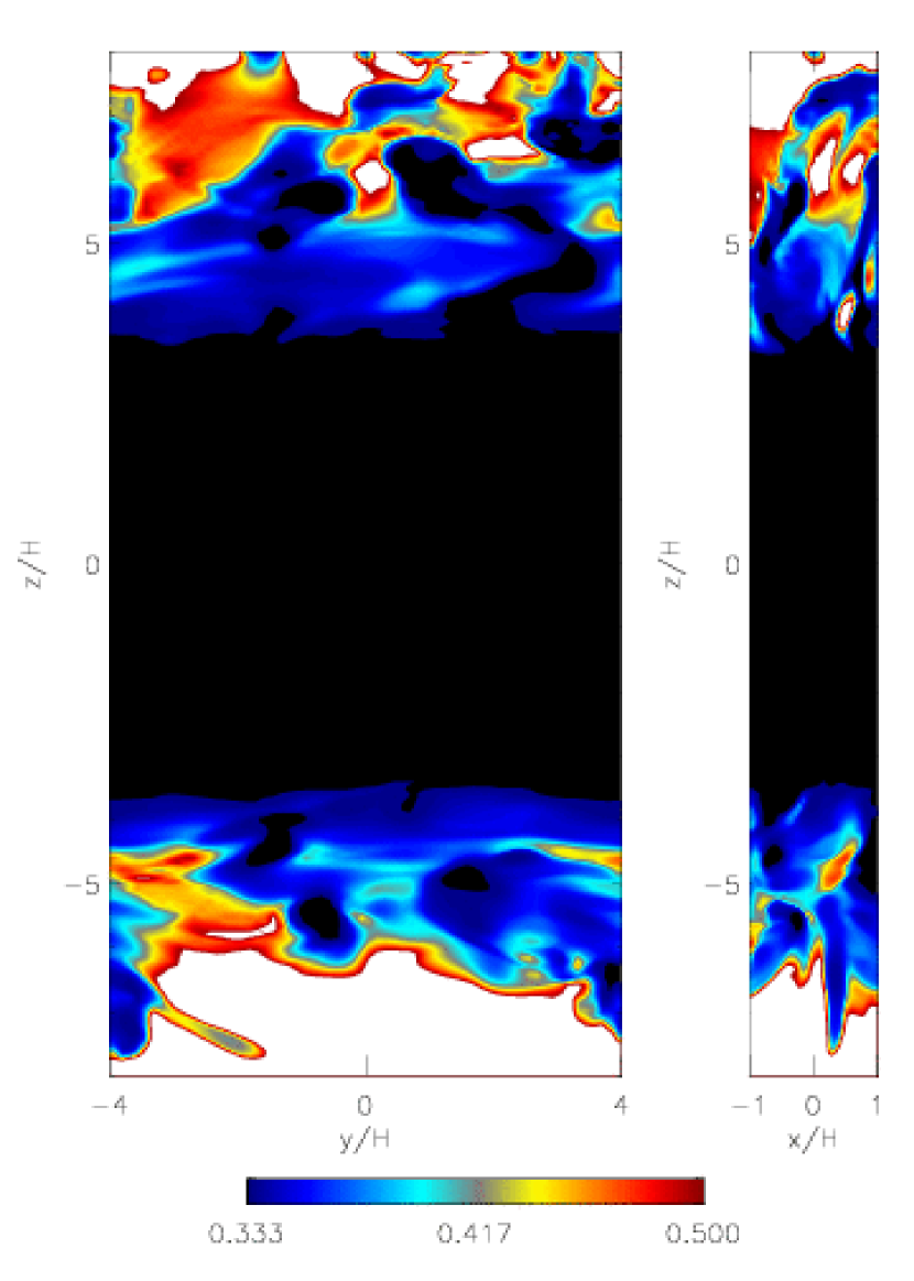
Figure 11: Left panel: The Eddington factor in two vertical planes at $t=32$ orbits. In all the white regions, the photons are better described as free-streaming than diffusing. Right panel: The horizontally-averaged photospheric altitude as a function of time.

One of the goals of this effort was to compute the structure of the disk all the way from the midplane out through the photosphere so that we could truly say we were describing the entire flow of radiation energy through the disk. Figure 11 shows the extent to which we succeeded in reaching this goal. In its left-hand panel, we show a snapshot of the Eddington factor $f$ as a function of position in the $x-z$ and $y-z$ planes. Deep within the optically-thick disk, the photon intensity is isotropic and $f=1/3$; far above the photosphere, the photons become nearly mono-directional and $f\rightarrow 1$. We choose to define the photospheric level as the place at which $f=1/2$. By this standard, we see that the photospheric surface at any given time is highly irregular. Its height above the midplane can be anywhere from $\simeq 6.5H$ to outside $\geq 8H$. In fact, there are places where, as a function of $z$, the photon distribution appears to pass back and forth with increasing altitude from nearly free-streaming to more nearly diffusive.

The snapshot shows roughness in the photospheric surface at a fixed time. Some of the fluctuations are correlated in time, so that the horizontal mean level of the photosphere also moves up and down over time (as portrayed in the right-hand panel of Fig. 11). In this horizontally-averaged sense, the photosphere generally varies between $6.5H$ and $8H$ from the midplane, but there are occasional excursions both to slightly lower and somewhat greater altitude. The duration of these fluctuations can vary from a small fraction of an orbit to 1–2 orbits. We caution, however, that our method of photosphere determination somewhat overestimates its height from the midplane during times when the density in the outer portion of the box is consistently at the floor. Examples of such times can be identified in the right-hand panel of Figure 11 as those periods during which the nominal photospheric altitude is constant at $\simeq 6.5H$. The fact that the density floor is always the same accounts for the constancy of the estimated photospheric height during these periods.

3.3 Internal Fluctuations

MHD turbulence is, of course, at the heart of the dynamics in this system. As a result, fluctuations are central. We find that the character of these fluctuations is a strong function of altitude from the midplane (Fig. 12). Because virtually every quantity has a strong systematic dependence on $|z|$, we define all fluctuations as relative to the mean at a given height.

3.3.1 Gas density and magnetic intensity

The gas is almost incompressible near the midplane, but the amplitude of density fluctuations grows rapidly up to $|z|\simeq 6H$, and declines even more sharply out to the top of the box. Near $|z|\simeq 6H$, the rms fractional fluctuation can be anywhere from $\simeq 1$–4 (at the time shown in Fig. 12 it is $\simeq 2.5$). By contrast, the magnetic field strength behaves in exactly complementary fashion: with the exception of some likely spurious fluctuations associated with the boundaries, it fluctuates the most in the densest part of the disk, $|z|\leq 2.5H$.

This behavior corresponds to the varying value of the plasma $\beta$ defined in terms of the sum of gas and radiation pressure. Where $\beta$ is large (near the midplane), magnetic effects cannot compress the gas; where it is small (roughly $2.5H\lesssim z\lesssim 7H$), magnetic forces can be very effective in driving gas compression and rarefaction. Large opacity guarantees such a strong dynamical coupling between gas and radiation that their pressures sum for the purpose of resisting magnetically-driven compression except on very small scales far from the midplane.

3.3.2 Velocity

Velocity fluctuations behave in a manner similar to density fluctuations. In absolute terms, the largest random speeds are seen at high altitudes, $|z|>5H$. In terms of the Mach number relative to the magnetosonic speed (i.e., $c_{s}^{2}\equiv[(5/3)p+(4/3)p_{\rm rad}+2p_{\rm mag}]/\rho$), the random motions are $\sim 0.3$ over most of the volume, but can sometimes increase to $\sim 1$–2 near one or the other boundary.

This behavior is qualitatively similar to what was seen in the simulations of Miller & Stone (2000). They found that, measuring Mach number relative to the gas sound speed alone, the rms fluid speed rose from $\simeq 0.15$ in the midplane to $\sim 1$ near the outer boundaries. Although the actual fluid speeds we see are considerably greater than the gas sound speed, their Mach number with respect to the total sound speed is about the same.

3.3.3 Temperature

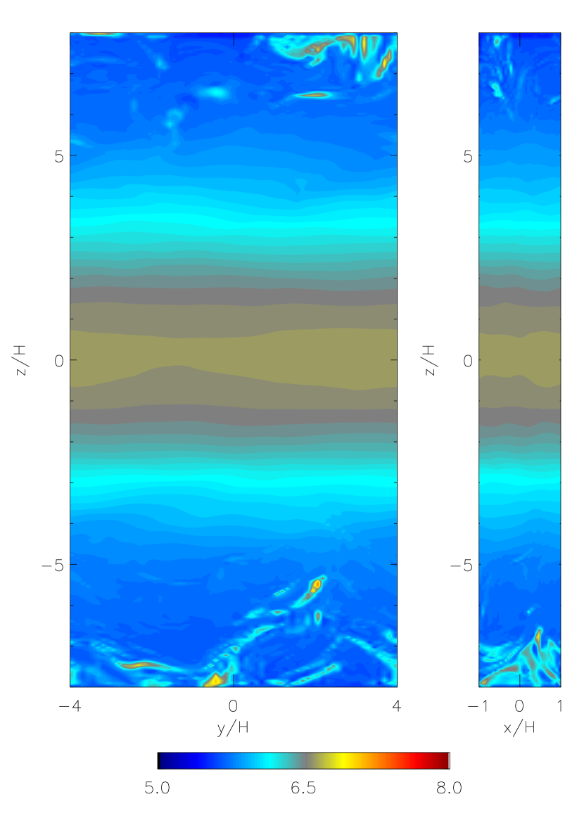
Figure 13: Temperature on a logarithmic scale in two vertical planes at time $t=25$ orbits.

In the disk body, the temperature is generally quite uniform at any given altitude. However, in the region above $5H$, at any given time there is generally a few percent of the volume in which the temperature is elevated by a factor of 5 or so above the mean (Fig. 13). Strong negative fluctuations are quite rare. Most often these regions of elevated temperature are roughly round, anywhere from $0.1H$ to $0.5H$ in diameter (so the larger ones are well-resolved by our grid), but occasionally they can be sheet-like.

3.3.4 Top-bottom asymmetry

A different sort of fluctuation may be seen in space-time plots. Although in the long-run the top and bottom halves of the disk behave symmetrically, as shown in Figure 14, the magnetic field can be persistently stronger on one side of the midplane than on the other. Because energy dissipation is largely magnetic, during periods of asymmetry in field strength there is generally a corresponding asymmetry in dissipation rate. Moreover, the fact that much of the dissipation takes place several scale-heights from the midplane means that an asymmetry in dissipation is mirrored in a dissipation in flux. For periods as long as 5–10 orbits, the radiation flux through the top or bottom surface can be as much as 2–3 times as much as through the opposite surface (Fig. 15), although through most of the simulation the contrast was smaller, typically $\sim$ 20%.

3.4 Magnetic fieldline structure

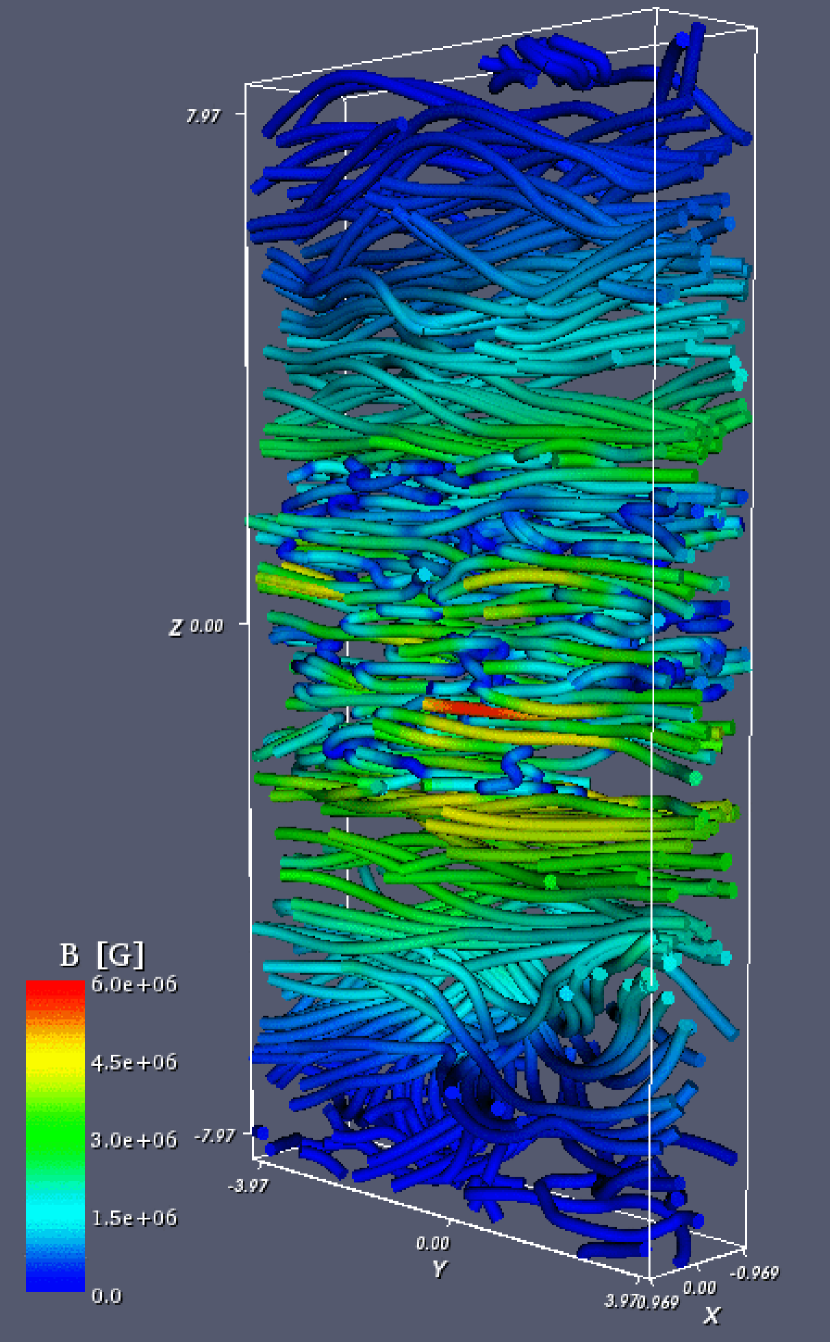
Figure 16: Magnetic field structure at $t=25$ orbits. Color represents the magnitude of the magnetic field in Gauss. Starting points of field-line integrations are randomly distributed in the box, and thus the density of field-lines is not proportional to the magnitude.

A view of the magnetic field structure in the steady state is shown in Figure 16. The field-lines are predominantly azimuthal throughout the box, but subtle differences can be distinguished as a function of altitude. Near the midplane ($|z|<2H$), the field-lines are tangled on short scales ($\sim 0.1H$), corresponding to the MHD turbulence driven by the MRI. At mid-altitudes ($2H<|z|<5H$), the field-lines are generally fairly smooth. In the high-altitude zone ($5H<|z|$), the field-lines get disordered again, and the scale of wiggles is larger ($\sim H$) compared to that near the midplane. This is because random fluid motions are powerful enough (see section 3.3.2) to substantially perturb fieldlines.

4 Discussion

4.1 What is a corona?

Perhaps the most striking structural feature apparent in this simulation is the $|z|>3H$ region, where most of the support against gravity is from magnetic pressure. On the basis of its low plasma $\beta$, it might be described as a corona, but it is a very unusual corona in that it lies well below the photosphere. Because of this magnetic support, the top surface of the disk (if “top” is defined as the photosphere), is considerably higher above the midplane than where the disk surface is conventionally estimated to be. An isothermal Gaussian model, for example, places the photosphere at merely $3H$, rather than $>7H$ as we find. Although a similarly magnetically-supported region existed in the Miller & Stone (2000) simulations, it went unremarked because they did not evaluate the optical depth.

The nature of this region also contradicts another frequently-held view: that magnetically-dominated layers at high altitude should be the site of intense heating, so intense that the temperature can be raised high enough to support hard X-ray emission. This idea was given indirect support by the Miller & Stone (2000) finding of substantial vertical Poynting flux in the region a few scale-heights from the midplane, although they could not test it directly because they assumed an isothermal equation of state. We find rather less Poynting flux than did they, and little heat dissipation in the magnetically-dominated region.

The absence of dissipation in the “corona” is most likely a result of the very fact that this zone is magnetically-dominated: the field smooths itself. We do see a narrow zone of high dissipation rate immediately inside the outer boundaries, and the dissipation there does raise the temperature by about a factor of two, but at least part (and maybe all) of this heating near the boundary is likely to be a numerical artifact. We also observe transient localized regions of very high temperature in this “corona” well below the outer boundary, but these are neither hot enough nor common enough to count for much in terms of global properties.

These results raise the question of where the observed hard X-rays are made. Perhaps more promising sites for their production can be found at smaller radii. Where radiation pressure dominates gas pressure at all altitudes, the disk’s internal vertical profile may be very different. In addition, as demonstrated in Hirose et al. (2004), there can be extremely high current-density regions at radii comparable to or smaller than the marginally stable orbit and well away from the equatorial plane. Hirose et al. speculated that these, too, may be loci of hard X-ray production.

4.2 Observed radiation

In comparison to the commonly-assumed Gaussian density profile, the extended magnetically-supported atmosphere found in our simulation can be expected to alter the locally-emitted spectrum in significant ways. Specifically, the very steep density gradient at the photosphere predicted by the Gaussian model entails a large density there. In the lower density environment we find near the photosphere, larger departures from LTE might be expected, and therefore stronger non-thermal features in the emergent spectrum. A symptom that something of this sort may happen can be seen in the band, a few scale-heights thick, in which the gas temperature rises well above the local radiation temperature.

In the great majority of atmosphere calculations, whether in the context of stars or accretion disks, it is assumed that the photospheric region may be approximated as time-steady and having 1-d slab geometry. Our results regarding both the location of the photosphere and temperature fluctuations in the upper disk call both approximations into question. However, the nature of radiation transfer may ameliorate both problems. Because the photon diffusion time is very short compared to the local dynamical time in the upper atmosphere of the disk, the radiation can respond very quickly to varying conditions. The nature of its response is for diffusion to smooth out irregularities; in fact, there is far less spatial variation in horizontal planes in the radiation intensity than in the gas density or temperature or magnetic field strength (Fig. 12). In addition, the characteristic temperature fluctuation takes the form of a spot of high temperature, but because the opacity diminishes with increasing temperature, these spots largely decouple from the radiation.

Another virtually universal assumption made in previous work on accretion disks is that their top and bottom surfaces should have equal surface brightness. Yet we find that the magnetic field intensity, and therefore the dissipation rate, and consequently the emergent flux, can be asymmetric with respect to the midplane with a consistent sense of contrast for as long as 5–10 orbits at a stretch. Because we are simulating a shearing-box and not an entire disk, we have no way of knowing how well correlated such asymmetries might be in radius. If there is significant coherence in these fluctuations over radial extents comparable to the local radius, the luminosity of the disk as measured by any single observer could be wrong by factors of a few.

It is likewise frequently asserted that the radiation from a disk surface cannot vary in any substantial way on timescales shorter than a cooling time. We have found, however, that because so much of the dissipation variation takes place at comparatively high altitude, it is entirely possible for the emergent flux to vary as much as an order of magnitude faster than the global equilibration cooling time.

4.3 Scaling with central mass

Most properties of accretion disks depend only on quantities such as the accretion rate in Eddington units $\dot{m}$ and the radius in gravitational radii from which the mass of the central object has already been scaled out. However, the temperature is different. For fixed $\dot{m}$ and $r/r_{g}$, the temperature is $\propto M^{-1/4}$. The most significant effects that this is likely to have on the properties discussed here all result from the dependence of the opacity on temperature.

As we mentioned earlier, we chose a relatively small central mass ($6.6M_{\odot}$) so that sources of opacity other than free-free absorption and Thomson opacity would be comparatively unimportant. However, if the mass were $\sim 10^{5}$ times greater, with $\dot{m}$ and $r/r_{g}$ fixed at the values of our simulation (0.1 and 300), the surface temperature would fall to $\simeq 4\times 10^{4}$ K. At this temperature, there would be substantial opacity due to resonance lines in medium-$Z$ elements. It is possible that the scattering opacity would then be so large that the vertical radiation force could overcome the vertical component of gravity even at high altitude (cf. Proga & Kallman 2004). In this circumstance, the vertical structure of the disk would undoubtedly be quite different.

In a similar vein, at still higher masses ($\sim 10^{8}M_{\odot}$, the domain of AGNs), the surface temperature would be $\simeq 1\times 10^{4}$ K, where ionization transitions can lead to pulsational instabilities.

5 Conclusions

We have shown that it is now possible to track in some detail the path of energy within accretion disks, from turbulent dissipation to heat to diffusing photons. When we do so, we find that some conclusions about disk structure drawn on simpler thermodynamic models (e.g., isothermal equations of state) are supported, but not all. For example, the existence of an extended magnetically-supported atmosphere was already predicted by the isothermal models. What they could not do, however, because they did not compute optical depths, was to discover that a large part of this magnetically-supported atmosphere can lie below the photosphere.

Our model for the dissipation of turbulence will certainly not be the final word on this subject—we do not have the resolution to capture the full inertial range of MHD turbulence driven by the MRI, nor do we compute its genuine microphysics. However, locating dissipation where the gradients are so sharp as to cause numerical losses of magnetic and kinetic energy is a very plausible supposition. On the basis of this method, we have found that the time-averaged dissipation profile is roughly flat in terms of rate per unit volume within roughly $\pm 3H$ of the midplane, but drops sharply outside that height, with very little dissipation in the magnetically-supported (but optically-thick) “corona”. Over timescales that are presumably short compared to the lifetime of the disk, but comparable to or even somewhat greater than the local cooling time, there can be sizable departures from this mean profile, especially in the sense of an asymmetry between the top and bottom halves of the disk.

We have also found that this spread in the dissipation permits significant parts of it to be found in places where the photon diffusion time to the surface is relatively short. Consequently, there can be significant fluctuations in the outgoing flux that track fluctuations in the disk heating rate with a lag that is an order of magnitude shorter than the nominal cooling time.

Lastly, the detailed structure we have computed suggests that the emergent spectrum from the gas-dominated portions of accretion disks may deviate significantly from blackbody. They are likely to have extended atmospheres in which the gas temperature differs from the radiation temperature and the densities are low enough that other breakdowns in the details of LTE may occur. In addition, the photospheric surface itself may have both a complicated topology and interesting fluctuations, leading to additional non-blackbody effects.

Appendix A Implementation of Total Energy Conservation

A.1 Operator-splitting

The numerical scheme of the ZEUS code, upon which our code is built, consists of the following seven steps:

1. source step (inertial and gravitational part)

   $$\frac{\partial\mbox{\boldmath$v$}}{\partial t}=-2\rho\left(\Omega\hat{\mbox{\boldmath$z$}}\right)\times\mbox{\boldmath$v$}+3\rho\Omega^{2}x\hat{\mbox{\boldmath$x$}}-\rho\Omega^{2}z\hat{\mbox{\boldmath$z$}}$$ (A1)

2. source step (radiation part)

   $$\frac{\partial\mbox{\boldmath$v$}}{\partial t}=-\frac{\chi\rho}{c}\mbox{\boldmath$F$}$$ (A2)

   $$\frac{\partial e}{\partial t}=-\left(4\pi B-cE\right)\kappa\rho$$ (A3)

   $$\frac{\partial E}{\partial t}=\left(4\pi B-cE\right)\kappa\rho-\mathsf{P}:\nabla\mbox{\boldmath$v$}$$ (A4)

3. radiation diffusion

   $$\frac{\partial E}{\partial t}+\nabla\cdot\mbox{\boldmath$F$}=0$$ (A5)

4. gas pressure gradient

   $$\frac{\partial\mbox{\boldmath$v$}}{\partial t}=-\frac{\nabla p}{\rho}$$ (A6)

   $$\frac{\partial e}{\partial t}=-p\left(\nabla\cdot\mbox{\boldmath$v$}\right)$$ (A7)

5. artificial viscosity

   $$\frac{\partial\mbox{\boldmath$v$}}{\partial t}=-\frac{\nabla q}{\rho}$$ (A8)

   $$\frac{\partial e}{\partial t}=-q\left(\nabla\cdot\mbox{\boldmath$v$}\right)$$ (A9)

6. transport step

   $$\frac{\partial\rho}{\partial t}+\nabla\cdot\left(\rho\mbox{\boldmath$v$}\right)=0$$ (A10)

   $$\frac{\partial\rho\mbox{\boldmath$v$}}{\partial t}+\nabla\cdot\left(\rho\mbox{\boldmath$v$}\mbox{\boldmath$v$}\right)=0$$ (A11)

   $$\frac{\partial E}{\partial t}+\nabla\cdot\left(E\mbox{\boldmath$v$}\right)=0$$ (A12)

   $$\frac{\partial e}{\partial t}+\nabla\cdot\left(e\mbox{\boldmath$v$}\right)=0$$ (A13)

7. magnetic part

   $$\frac{\partial\mbox{\boldmath$v$}}{\partial t}=\frac{1}{\rho}\mbox{\boldmath$j$}\times\mbox{\boldmath$B$}$$ (A14)

   $$\frac{\partial\mbox{\boldmath$B$}}{\partial t}+\nabla\times\mbox{\boldmath$E$}=0$$ (A15)

   $$\frac{\partial e}{\partial t}=0$$ (A16)

To transform this into an energy-conserving numerical scheme, several changes are required. Turner et al. (2003) began this transformation by altering step 7 to be the solution of a total energy equation in the conservative form

$$\frac{\partial}{\partial t}\left(\frac{1}{2}\rho\mbox{\boldmath$v$}^{2}+e+\frac{1}{8\pi}\mbox{\boldmath$B$}^{2}\right)+\nabla\cdot\left(\frac{1}{4\pi}\mbox{\boldmath$E$}\times\mbox{\boldmath$B$}\right)=0.$$ (A17)

They then updated the internal energy according to

$$e^{*}=\left(\rho\frac{\mbox{\boldmath$v$}^{2}}{2}+e+\frac{\mbox{\boldmath$B$}^{2}}{8\pi}\right)^{*}-\left(\rho^{*}\frac{{\mbox{\boldmath$v$}^{*}}^{2}}{2}+\frac{{\mbox{\boldmath$B$}^{*}}^{2}}{8\pi}\right),$$ (A18)

where the asterisk variables denote those updated in the step. In this way, any kinetic or magnetic energy that might have been lost numerically during this step is instead captured into internal energy because the total energy $\rho\mbox{\boldmath$v$}^{2}/2+e+\mbox{\boldmath$B$}^{2}/(8\pi)$ is conserved.

We have extended this approach to steps 4, 5, and 6, in order to capture in the same way any kinetic energy that would otherwise be lost. In each of these steps, the internal energy equation is replaced by the corresponding total energy equation:

1. gas pressure gradient

   $$\frac{\partial}{\partial t}\left(\frac{1}{2}\rho\mbox{\boldmath$v$}^{2}+e\right)+\nabla\cdot\left(p\mbox{\boldmath$v$}\right)=0$$ (A19)

2. artificial viscosity

   $$\frac{\partial}{\partial t}\left(\frac{1}{2}\rho\mbox{\boldmath$v$}^{2}+e\right)+\nabla\cdot\left(q\mbox{\boldmath$v$}\right)=0$$ (A20)

3. transport step

   $$\frac{\partial}{\partial t}\left(\frac{1}{2}\rho\mbox{\boldmath$v$}^{2}+e\right)+\nabla\cdot\left\{\left(\frac{1}{2}\rho\mbox{\boldmath$v$}^{2}+e\right)\mbox{\boldmath$v$}\right\}=0$$ (A21)

After each of these steps, the internal energy is updated by

$$e^{*}=\left(\rho\frac{\mbox{\boldmath$v$}^{2}}{2}+e\right)^{*}-\left(\rho^{*}\frac{{\mbox{\boldmath$v$}^{*}}^{2}}{2}\right).$$ (A22)

Thus, the kinetic and magnetic energies that in the original ZEUS code would be lost numerically are completely captured as internal energy during steps 4 to 7 in our scheme. The net result of all these steps is represented by the symbol $Q$ in Equation 5. We show how it is explicitly computed in Appendix A.2.

A.2 Dissipation rate

The dependent variables $e$, $E$, $\rho$, $B$, and $v$ suffice to determine the state of the simulation. However, we are interested in the dissipation as a function of time and position as a fundamental diagnostic of the thermal physics in these disks. Because of the way we update the internal energy, to record the dissipation rate requires some special effort.

The total dissipation rate receives contributions in all the steps from 4 through 7. To compute their individual rates, we retain the internal energy equation and solve it in parallel with the total energy equation. At each step, we must distinguish between the internal energy as it evolves and the internal energy that would have resulted from adiabatic changes alone. For the purposes of this discussion, we convey this distinction by defining $e$ as the internal energy before an update step, $e^{*}$ as the internal energy after update by the total energy equation, and $\tilde{e}^{*}$ as the internal energy after an update by the internal energy equation alone.

The artificial viscosity dissipation rate in step 5 can be computed as $(\tilde{e}^{*}-e)/\Delta t$ because the RHS of the internal energy equation in this step is nothing more than this dissipation rate. On the other hand, the numerical dissipation rate in each of steps 4 through 7 can be evaluated as $(e^{*}-\tilde{e}^{*})/\Delta t$ because the difference $e^{*}-\tilde{e}^{*}$ corresponds to the numerically-lost kinetic and magnetic energies captured as internal energy.

The total dissipation rate in the simulation can then be written as the sum of all these rates:

$$Q=\left.{\frac{\tilde{e}^{*}-e}{\Delta t}}\right|_{\rm step=5}+\sum_{\rm step=4,5,6,7}\frac{e^{*}-\tilde{e}^{*}}{\Delta t}.$$ (A23)

Note that the artificial viscosity dissipation rate $(\tilde{e}^{*}-e)/\Delta t$ is always positive by definition, whereas a numerical dissipation rate $(e^{*}-\tilde{e}^{*})/\Delta t$ can be negative due to numerical errors.

Because our evaluation of the dissipation rate intrinsically involves capturing numerical errors that are likely to depend strongly on the grid-scale relative to the scale of physical gradients, one might fairly ask whether our results are sensitive to resolution. To answer this question, we have run a shorter simulation with a grid having twice the resolution in the $y$-direction. The initial condition for this resolution-testing simulation was the state of the main simulation at $t=35$ orbits, and it ran for 1 full orbit. To distinguish the two, we call our primary simulation the “standard”.

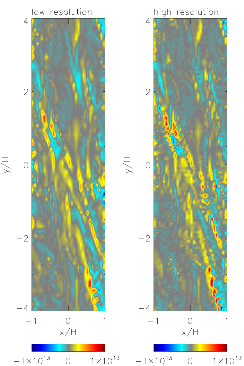
Figure 17: Left panel: Dissipation rate per unit volume at $z=0$ and $t=35.1$ orbits in the standard simulation (left-hand image) and the high-resolution simulation (right-hand image). Right panel: Volume-integrated dissipation rate for the standard simulation (solid curve) and high-resolution simulation (dotted curve).

For times up to a few tenths of an orbit after its start, the distribution of dissipation in the higher-resolution simulation remained very similar to that in the standard one with the exception that peaks in the dissipation were more sharply-defined (Fig. 17). After a few tenths of an orbit, the chaotic character of the turbulent dynamics leads to a divergence of the detailed structure of the flow as compared to the standard simulation. Nonetheless, the time-history of the volume-integrated dissipation rate in the higher-resolution simulation tracks closely that of the standard for the duration of the test, deviating by only a few percent at most over an orbital period. Thus, we conclude that if the magnetic structure is independently fixed in place, our numerical scheme locates the dissipation more or less as well as it can, given the constraints posed by the actual resolution employed. Over timescales long enough to move the specific places where dissipation happens, the fact that the volume-integrated dissipation rate hardly changes in this limited resolution test means that we have no immediate grounds for concern about sensitivity of our results to our resolution scale.

A.3 Artificial energy injection

Three limiting values must be placed on quantities in order to preserve stability and to keep the time-step from becoming prohibitively small. These are: a density floor, an energy floor, and a velocity cap. The density floor and the velocity cap are applied only after step 7, but the energy floor is applied in each of steps 4 to 7. Here we describe how they work and evaluate energy injection rates associated with each of them.

(a) density floor: An extremely low density would cause a very short time-step because $\Delta t$ must be $<\Delta x/c_{\rm ms}$. If the density were to go negative, it could cause the code to halt. To avoid either of these problems, the density $\rho$ is set to the floor value $\rho_{\rm floor}$ when $\rho<\rho_{\rm floor}$. For this simulation, we set $\rho_{\rm floor}$ to $10^{-5}$ times the initial density at the midplane. The energy injection rate due to the density floor is

$$S_{1}\equiv\cases{(\rho_{\rm floor}\mbox{\boldmath$v$}^{2}/2-\rho\mbox{\boldmath$v$}^{2}/2)/\Delta t&(if $\rho<\rho_{\rm floor}$)\cr 0&(otherwise).}$$ (A24)

(b) energy floor: The internal energy computed by the total energy equation, $e^{*}$, can become extremely small or even negative due to numerical errors. Simply applying a floor of small value does not work because it can lead to an unphysically large free-free opacity. Therefore, we employ $\tilde{e}^{*}$ instead of $e^{*}$ when $e^{*}<f\tilde{e}^{*}$; the fudge factor $f=0.5$ in this simulation. The energy injection rate is then

$$S_{2}\equiv\cases{\sum_{\rm step=4}^{7}(\tilde{e}^{*}-e^{*})/\Delta t&(if $e^{*}<f\tilde{e}^{*}$)\cr 0&(otherwise).\cr}$$ (A25)

(c) velocity cap: Two different limits are placed on the velocity: (1) To avoid inflows through the top and bottom boundaries, the $z$-component of the velocity at the top (bottom) boundary surfaces is forced to zero when it is negative (positive). (2) To avoid unusually large speeds due to numerical errors, a cap is applied to the magnitude of each component of the velocity; the value of the velocity cap is set to $10(3/2)\Omega L_{x}$, where $L_{x}$ is the full-width of the box in the $x$-direction. The energy injection rate due to these corrections is

$$S_{3}\equiv\cases{(\rho\mbox{\boldmath$v$}_{\rm corrected}^{2}/2-\rho\mbox{\boldmath$v$}^{2}/2)/\Delta t&(if $\mbox{\boldmath$v$}$ is corrected)\cr 0&(otherwise),}$$ (A26)

which is always negative by definition.

Integrated over the 60 orbits of the simulation, each of these is quite small, but the total amounts of energy injection due to the energy floor and velocity cap are rather smaller than that due to the density floor. Relative to the total dissipated energy, the density floor adds 0.9%, the energy floor subtracts 0.06%, and the velocity cap subtracts 0.05%.

A.4 Testing energy conservation

Total energy conservation in our system can be written as follows.

$$\frac{\partial\mathcal{E}}{\partial t}+\nabla\cdot\mbox{\boldmath$\mathcal{F}$}=\mathcal{S}$$ (A27)

$$\quad\mathcal{E}\equiv\frac{1}{2}\rho\mbox{\boldmath$v$}^{2}+e+\frac{1}{2}\mbox{\boldmath$B$}^{2}+E$$ (A28)

$$\quad\mbox{\boldmath$\mathcal{F}$}\equiv\left(\frac{1}{2}\rho\mbox{\boldmath$v$}^{2}+e\right)\mbox{\boldmath$v$}+\left(p+q\right)\mbox{\boldmath$v$}+\mbox{\boldmath$E$}\times\mbox{\boldmath$B$}+E\mbox{\boldmath$v$}+\mbox{\boldmath$F$}$$ (A29)

$$\quad\mathcal{S}\equiv\left\{-2\rho\left(\Omega\hat{\mbox{\boldmath$z$}}\right)\times\mbox{\boldmath$v$}+3\rho\Omega^{2}x\hat{\mbox{\boldmath$x$}}-\rho\Omega^{2}z\hat{\mbox{\boldmath$z$}}\right\}\cdot\mbox{\boldmath$v$}+\left(\frac{\chi\rho}{c}\mbox{\boldmath$F$}\right)\cdot\mbox{\boldmath$v$}-\mathsf{P}:\nabla\mbox{\boldmath$v$}$$

$$\qquad+S_{1}+S_{2}+S_{3}$$ (A30)

Integrating equation (A27) over time and volume, we have

$$\bar{\mathcal{E}}(t)=\bar{\mathcal{E}}(0)+\int_{0}^{t}\,dt^{\prime}\left\{-\bar{\mathcal{F}}(t^{\prime})+\bar{\mathcal{S}}(t^{\prime})\right\},$$ (A31)

where $\bar{\mathcal{E}}$, $\bar{\mathcal{F}}$, and $\bar{\mathcal{S}}$ are, respectively, volume integrals of $\mathcal{E}$, $\nabla\cdot\mbox{\boldmath$\mathcal{F}$}$, and $\mathcal{S}$. To evaluate how well total energy is conserved in our numerical code, we computed a relative error $({\rm LHS}-{\rm RHS})/{\rm LHS}$ as a function of time, which is shown in Figure 18. We see that the absolute value of the error stays lower than $0.1\%$ over a span of 60 orbits.

Appendix B Boundary Condition for Radiation Diffusion Equation

The top and bottom boundary conditions for the radiation diffusion equation (step 3 in Appendix A) are determined by a requirement that the diffusion flux $F_{z}=-DdE/dz$ across the boundary is equal to that across the adjacent cell surface. Here the diffusion coefficient $D\equiv c\Lambda/(\chi\rho)$. We implement this condition by the following procedure (Turner, 2004): First, we assume that the requirement holds exactly at the previous step,

$$-D_{i,j,k+1/2}^{n-1}\frac{E_{i,j,k+1}^{n-1}-E_{i,j,k}^{n-1}}{\Delta z}=-D_{i,j,k-1/2}^{n-1}\frac{E_{i,j,k}^{n-1}-E_{i,j,k-1}^{n-1}}{\Delta z},$$ (B1)

where $n$, $i$, $j$, and $k$ denote respectively the time step number and the grid indexes in the $x$-, $y$-, and $z$-directions. Hereafter we omit the inactive indices $i$ and $j$ for clarity. Then, we compute the ratio of radiation energy in the ghost cell (index $k+1$) to that in the last real cell (index $k$) from the above equation,

$$r\equiv\frac{E_{k+1}^{n-1}}{E_{k}^{n-1}}=1+\frac{D_{k-1/2}^{n-1}}{D_{k+1/2}^{n-1}}\left(1-\frac{E_{k-1}^{n-1}}{E_{k}^{n-1}}\right).$$ (B2)

Finally, assuming that the ratio $r$ changes slowly over time, we obtain the boundary condition for the radiation energy in the current step,

$$E_{k+1}^{n}=rE_{k}^{n}.$$ (B3)

Therefore, the requirement holds only approximately in the current step. However, this boundary condition is stable and also easy to implement in the numerical code.

Figure 1: Horizontally-averaged density: initial condition (thin curve) and time-averaged profile (thick curve).

Figure 2: Left panel: horizontally-averaged pressure. All initial condition curves are thin, all time-averaged curves are thick. In each case, gas pressure is represented by a dot-dash curve, magnetic pressure by a solid curve, and radiation pressure by a dotted curve. Right panel: time- and horizontally-averaged contributions to net vertical acceleration. Gravity is shown by a dashed curve, other quantities by the same line-styles as in the left-hand panel.

Figure 3: Temperature as a function of height. Gas temperature is shown by the solid curves, heavy for the time-averaged profile, thin for the initial condition; time-averaged radiation temperature is shown by the dotted curve.

Figure 4: Work done on radial surfaces (solid), outgoing energy through top and bottom boundaries (dotted), and artificial energy injection, i.e., $S_{1}+S_{2}+S_{3}$ as defined in Appendix A.3 (thin solid), all as functions of time.

Figure 5: Time- and horizontally-averaged dissipation as a function of height within the disk (solid curve). Stress multiplied by $(3/2)\Omega$ is shown with a dotted curve.

Figure 6: The outward energy flux (i.e., flux directed away from the midplane) carried by radiation (solid curve), Poynting flux (dash-dot curve), and convective gas motions (dashed curve). The units of flux are erg cm^-2 orbit^-1.

Figure 7: Volume-integrated dissipation as a function of time (solid curve) and volume-integrated $x$–$y$ stress multiplied by $(3/2)\Omega$ (dashed curve).

Figure 10: Cross-correlation between volume-integrated dissipation rate and outgoing flux.

Figure 12: RMS fractional fluctuation as a function of altitude at $t=25$ orbits. Heavy solid line: gas density; thin solid line: magnetic field intensity; dotted line: radiation energy.

Figure 15: Radiation flux leaving the top (solid curve) and bottom (dotted curve) surfaces as functions of time.

Figure 18: The energy conservation criterion described in text as a function of time through the simulation.

References

- Balbus & Hawley (1998) Balbus, S. A., & Hawley, J. F. 1998, Rev. Mod. Phys., 70, 1
- Brandenburg et al. (1995) Brandenburg, A., Nordlund, A., Stein, R.F. & Torkelsson, U. 1995, ApJ, 446, 741
- Hawley, Gammie, & Balbus (1995) Hawley, J.F., Gammie, C.F., & Balbus, S.A. 1995, ApJ, 440, 742
- Hawley & Krolik (2001) Hawley, J.F. & Krolik, J.H. 2001, ApJ, 548, 348
- Hirose et al. (2004) Hirose, S., Krolik, J. H., De Villiers, J.-P., & Hawley, J.F. 2004, ApJ, 606, 1083
- Ichimaru (1977) Ichimaru, S. 1977, ApJ, 214, 840
- Levermore & Pomraning (1981) Levermore, C.D. & Pomraning, G.C. 1981, ApJ, 248, 321
- Miller & Stone (2000) Miller, K. A., & Stone, J. M. 2000, ApJ, 534, 398
- Narayan & Yi (1994) Narayan, R. & Yi, I. 1994, ApJ, 428, L13
- Proga & Kallman (2004) Proga, D. & Kallman, T.R. 2004, ApJ, 616, 688
- Rees et al. (1982) Rees, M.J., Phinney, E.S., Begelman, M.C. & Blandford, R.D. 1982, Nature, 295, 17
- Shakura & Sunyaev (1973) Shakura, N.I. & Sunyaev, R.A. 1973, A&A, 24, 337
- Stone & Norman (1992a) Stone, J.M. & Norman, M.L. 1992, ApJS, 80, 753
- Stone & Norman (1992b) Stone, J.M. & Norman, M.L. 1992, ApJS, 80, 791
- Turner & Stone (2001) Turner, N.J., & Stone, J.M. 2001, ApJS, 135, 95
- Turner et al. (2003) Turner, N.J., Stone, J.M., Krolik, J.H., & Sano, T. 2003, ApJ, 593, 992
- Turner (2004) Turner, N.J. 2004, ApJ, 605, L45