Evidence for Fine Structure in the Chromospheric Umbral Oscillation

Abstract

Novel spectro-polarimetric observations of the He I multiplet are used to explore the dynamics of the chromospheric oscillation above sunspot umbrae. The results presented here provide strong evidence in support of the two-component model proposed by Socas-Navarro et al. According to this model, the waves propagate only inside channels of sub-arcsecond width (the “active” component), whereas the rest of the umbra remains nearly at rest (the “quiet” component). Although the observations support the fundamental elements of that model, there is one particular aspect that is not compatible with our data. We find that, contrarily to the scenario as originally proposed, the active component remains through the entire oscillation cycle and harbors both the upflowing and the downflowing phase of the oscillation.

1 Introduction

The chromospheric oscillation above sunspot umbrae is a paradigmatic case of wave propagation in a strongly magnetized plasma. This problem has drawn considerable attention both from the theoretical (e.g., Bogdan et al. 2003) and the empirical standpoint (Lites 1992 and references therein). An observational breakthrough was recently brought upon with the analysis of spectro-polarimetric data, which is providing exciting new insights into the process (Socas-Navarro et al. 2000a; Socas-Navarro et al. 2000b; Socas-Navarro et al. 2001; López Ariste et al. 2001; Centeno et al. 2005). Previously to these works, the chromospheric oscillation has been investigated by measuring the Doppler shift of line cores in time series of intensity spectra. A particularly good example, based on multi-wavelength observations, is the work of Kneer et al. (1981).

Unfortunately, spectral diagnostics based on chromospheric lines is very complicated due to non-LTE effects. Even direct measurements of chromospheric line cores are often compromised by the appearance of emission reversals associated with the upflowing phase of the oscillation, when the waves develop into shocks as they propagate into the less dense chromosphere. A very interesting exception to this rule is the He I multiplet at 10830 Å, which is formed over a very thin layer in the upper chromosphere (Avrett et al. 1994) and is not seen in emission at any time during the oscillation. These reasons make it a very promising multiplet for the diagnostics of chromospheric dynamics. However, there are two important observational challenges. First, the long wavelength makes this spectral region almost inaccessible to ordinary Si detectors (or only with a small quantum efficiency). Second, the 10830 lines are very weak, especially the blue transition which is barely visible in the spectra and is conspicuously blended with a photospheric Ca I line in sunspot umbrae.

In spite of those difficulties, there have been important investigations based on 10830 Stokes $I$ observations, starting with the pioneering work of Lites (1986). More recently, the development of new infrared polarimeters (Rüedi et al. 1995; Collados et al. 1999; Socas-Navarro et al. 2005a) has sparked a renewed interest in observations of the He I multiplet, but now also with full vector spectro-polarimetry. Centeno et al. (2005) demonstrated that the polarization signals observed in the 10830 region provide a much clearer picture of the oscillation than the intensity spectra alone. The sawtooth shape of the wavefront crossing the chromosphere becomes particularly obvious in fixed-slit Stokes $V$ time series.

Before the work of Socas-Navarro et al. (2000a), the chromospheric umbral oscillation was thought of as a homogeneous process with horizontal scales of several megameters, since these are the coherence scales of the observed spectroscopic velocities. However, those authors observed the systematic occurrence of anomalous polarization profiles during the upflowing phase of the oscillation, which turn out to be conspicuous signatures of small-scale mixture of two atmospheric components: an upward-propagating shock and a cool quiet atmosphere similar to that of the slowly downflowing phase. This small-scale mixture of the atmosphere cannot be detected in the intensity spectra, but it becomes obvious in the polarization profiles because the shocked component reverses the polarity of the Stokes $V$ signal. The addition of two opposite-sign profiles with very different Doppler shifts produces the anomalous shapes reported in that work.

The results of Socas-Navarro et al. (2000a), implying that the chromospheric shockwaves have spatial scales smaller than $\sim$1”, still await independent verification. In this work we looked for evidence in He I 10830 data to confirm or rebut their claim. It is important to emphasize that this multiplet does not produce emission reversals in a hot shocked atmosphere. Thus, one does not expect to observe anomalous profiles and the two-component scenario would not be as immediately obvious in these observations as it is in the Ca II lines.

Here we report on a systematic study of the polarization signal in the 10830 Å  spectral region, with emphasis on the search for possible signatures of the two-component scenario. We compared the observations with relatively simple simulations of the Stokes profiles produced by one- and two-component models. The results obtained provide strong evidence in favor of the two-component scenario and constitute the first empirical verification of fine structure in the umbral oscillation, using observations that are very different from those in previous works.

2 Observations

The observations presented here were carried out at the German Vacuum Tower Telescope at the Observatorio del Teide on 1st October 2000, using its instrument TIP (Tenerife Infrared Polarimeter, see Martínez Pillet et al. 1999), which allows to take simultaneous images of the four Stokes parameters as a function of wavelength and position along the spectrograph slit. The slit was placed across the center of the umbra of a fairly regular spot, with heliographic coordinates 11S 2W, and was kept fixed during the entire observing run ($\approx$ 1 hour). In order to achieve a good signal-to-noise ratio, we added up several images on-line, with a final temporal sampling of 7.9 seconds.

Image stability was achieved by using a correlation tracker device (Ballesteros et al. 1996), which compensates for the Earth’s high frequency atmospheric variability, as well as for solar rotation.

The observed spectral range spanned from 10825.5 to 10833 Å, with a spectral sampling of 31 mÅ per pixel. This spectral region includes three interesting features: A photospheric Si i line at 10827.09 Å, a chromospheric Helium i triplet (around 10830 Å), and a water vapour line (Rüedi et al. 1995) of telluric origin that can be used for calibration purposes, since it generates no polarization signal.

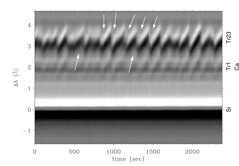
Figure 1: Stokes $V$ time series at a particular spatial position in the umbra of a sunspot. The labels on the right of the figure identify the spectral lines in the region shown. Wavelengths are measured in Å  from 10827. The arrows indicate where the rest Tr23 component might be (barely) visible under the oscillating component (see discussion in the text).

A standard reduction process was run over the raw data. Flatfield and dark current measurements were performed at the beginning and the end of the observing run and, in order to compensate for the telescope instrumental polarization, we also took a series of polarimetric calibration images. The calibration optics (Collados 1999) allows us to obtain the Mueller matrix of the light path between the instrumental calibration sub-system and the detector. This process leaves a section of the telescope without being calibrated, so further corrections of the residual cross-talk among Stokes parameters were done: the $I$ to $Q$, $U$ and $V$ cross-talk was removed by forcing to zero the continuum polarization, and the circular and linear polarization mutual cross-talk was calculated by means of statistical techniques (Collados 2003).

3 Interpretation

Let us first consider the relevant spectral features that produce significant polarization signals in the 10830 Å  region. The He multiplet is comprised of three different transitions, from a lower ${}^{3}S$ level with $J=0$ to three ${}^{3}P$ levels with $J=0,1$ and $2$. We hereafter refer to these as transitions Tr1, Tr2 and Tr3 for abbreviation. Tr2 (10830.25 Å) and Tr3 (10830.34 Å) are blended and appear as one spectral line (Tr23) at solar temperatures. Tr1 (10829.09 Å) is quite weak and relatively difficult to see in an intensity spectrum, while its Stokes $V$ signal can be easily measured. A photospheric Ca I line is seen blended with Tr1, but is only present in the relatively cool umbral atmosphere. Finally, a strong photospheric Si I line to the blue of Tr1 dominates the region both in the intensity and the polarized spectra.

When the time series of Stokes $V$ spectral images is displayed sequentially, one obtains a movie that shows the oscillatory pattern of the He lines. In the case of Tr1, the pattern is clearly superimposed on top of another spectral feature that remains at rest. This feature has the appearance of a broad spectral line with a core reversal similar to the magneto-optical reversal observed in many visible lines. Fig 1 shows the time evolution of Stokes $V$ at a particular spatial location in the umbra. The figure shows the oscillatory pattern superimposed to the motionless feature at the wavelength of Tr1 (we note that this is seen more clearly in the movies). In our first analyses, at the beginning of this investigation, we identified this feature at rest with the photospheric Ca line, which is not entirely correct as we argue below. It is likely that other authors have made the same assumption in previous works. We would like to emphasize that this static spectral feature under Tr1 is visible in all the temporal series of umbral oscillations we have so far (corresponding to different dates and different sunspots).

Some of the arguments discussed in this section are based on a Milne-Eddington simulation that contains all the transitions mentioned above. In the simulation, the He lines are computed taking into account the effects of incomplete Paschen-Back splitting (Socas-Navarro et al. 2004; Socas-Navarro et al. 2005b).

3.1 Tr1

Figure 1 reveals the sawtooth shape of the chromospheric oscillation in both Tr1 and Tr23, with a typical period of approximately 175 s . Every three minutes, the line profile undergoes a slow redshift followed by a sudden blueshift (the latter corresponding to material approaching the observer), resulting in the sawtooth shape of the oscillation observed in Figure 1. This dynamical behavior evidences shock wave formation at chromospheric heights. A detailed analysis is presented in Centeno et al (2005).

Looking closely at Tr1, one can see what at first sight would seem to be a photospheric umbral blend that does not move significantly during the oscillation. A search over the NIST (National Institute for Standards and Technology: http://www.physics.nist.gov) and VALD spectral line databases (Piskunov et al. 1995) produced only one possible match, namely the umbral Ca I line at 10829.27 Å. We initially identified this line with the blended feature because its wavelength, strength and umbral character (i.e., it is only observed in susnpot umbrae) were in good agreement with the data. However, when we tried to include this blend in our Stokes synthesis/inversion codes, it became obvious that something was missing in our picture.

The left panel of Fig 2 represents a portion of an observed time series at a fixed spatial point, with the lower part of the image replaced with profiles of the Si and Ca lines produced by our simulations. While the Si line appears to be correctly synthesized, the Ca line clearly differs from the observed profile. There are three noteworthy differences: a)The observed feature is much broader than the synthetic Ca line. b)The synthetic profile does not appear to be centered at the right wavelength. c)The observations exhibit a core reversal, very reminiscent of the well-known magneto-optical effects that are sometimes seen in visible lines.

We carried out more detailed simulations of the Ca line using an LTE code (LILIA, Socas-Navarro 2001). We synthesized this line in variations of the Harvard-Smithsonian reference atmosphere (HSRA, Gingerich et al. 1971) and the sunspot umbral model of Maltby et al. (1986). These were used to look for magneto-optical effects in the Stokes $V$ profiles and also to verify the width of the line shown in Fig 2 (left). We found that the LILIA calculations confirmed the line width and none of them showed any signs of Stokes $V$ core reversals. Thus, the discrepancy between the simulations and observations in the figure must be sought elsewhere.

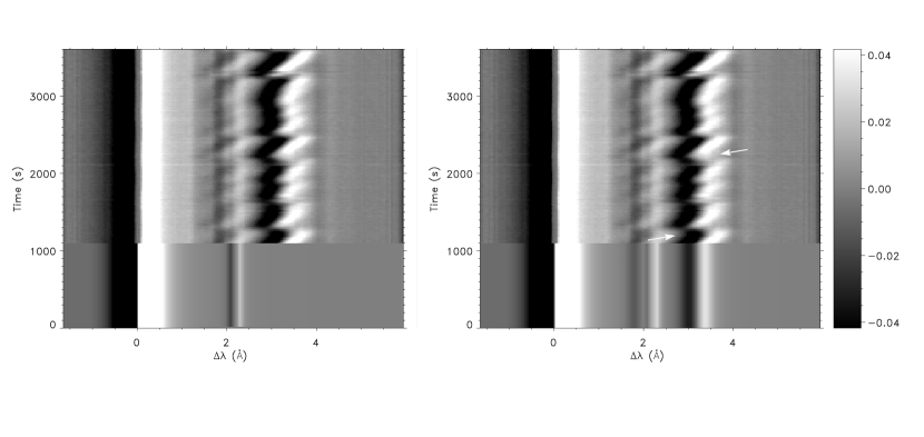
Figure 2: Similar to Figure 1, but the lower part of the image has been replaced by synthetic spectra. Left: Only the photospheric Si I and Ca I have been computed. Right: All four lines, including the He I multiplet, are computed in a quiet component (zero velocity). Note how this simulation reproduces the observed spectral feature at 10829 Å, including the core reversal. Wavelengths are measured in Å  from 10827. The arrows indicate where the rest Tr23 component might be (barely) visible under the oscillating component (see discussion in the text).

The right panel of Fig 2 shows the same dataset, again with the lower part replaced with a simulation. In this case the simulation contains, in addition to the photospheric Si and Ca lines, the He multiplet at rest. The synthesis was done with the incomplete Paschen-Back Milne-Eddington code. Note how the combination of Tr1 with the Ca line produces a spectral feature that is virtually identical to the observation, with the correct wavelength, width and even the core reversal. This scenario, with a quiet chromospheric component as proposed by Socas-Navarro et al. 2000a, naturally reproduces the observations with great fidelity. The core reversal arises then as the overlapping of the blue lobe of the Ca profile with the red lobe of Tr1.

3.2 Tr2

While Fig 2 presents a very convincing case in favor of the two-component scenario, one would like to see the quiet component also under the Tr23 line. Unfortunately, the simulations show that the quiet Tr23 profile must be obscured by the overlap with the active component. Only at the times of maximum excursion in the oscillation it might be possible to observe a brief glimpse of the hidden quiet component. One is tempted to recognize them in both Figs 1 and 2 (some examples are marked with arrows). Unfortunately, such features are too weak to be sure.

One might also wonder why the quiet component is rather obvious under Tr1 but not Tr23, since both lines form at approximately the same height and therefore have the same Doppler width. However, Tr23 is broader since it is actually a blend of two different transitions (Tr2 and Tr3) separated by $\sim$100 mÅ. Under typical solar conditions, the Doppler width of Tr1 in velocity units is $\sim$6 km s^-1. The width of Tr23, taking into account the wavelength separation of Tr2 and Tr3, is $\sim$9 km s^-1. Comparing these values to the amplitude of the chromospheric oscillation ($\sim$10 km s^-1), we can understand intuitively what the simulations already showed, namely that the quiet component may be observed under Tr1 but only marginally (if at all) under Tr23.

4 Conclusions

The observations and numerical simulations presented in this work indicate that the chromospheric umbral oscillation likely occurs on spatial scales smaller than the resolution element of the observations, or $\sim$1”. This suggests that the shock waves that drive the oscillation propagate inside channels within the umbra. Recent magneto-hydrodynamical simulations show that waves driven by a small piston in the lower atmosphere remain confined within the same field lines as they propagate upwards (Bogdan et al. 2003). This means that photospheric or subphotospheric small-scale structure is able to manifest itself in the higher atmosphere, even if the magnetic field is perfectly homogeneous.

The traditional scenario of the monolithic umbral oscillation, where the entire chromosphere moves up and down coherently, cannot explain earlier observations of the Ca II infrared triplet made by Socas-Navarro et al. (2000a). Our results using the He I multiplet support that view in that the active oscillating component occupies only a certain filling factor and coexists side by side with a quiet component that is nearly at rest. However, our observations refute one of the smaller ingredients of the model proposed by Socas-Navarro et al. (2000a), namely the disappearance of the active component after the upflow. In that work, the authors did not observe downflows in the active component. For this reason, they proposed that the oscillation proceeds as a series of jets that dump material into the upper chromosphere and then disappear. In our data we can see the Tr1 and Tr23 lines moving up and down in the active component, which seems to indicate that the active component remains intact during the entire oscillation cycle. Other than that, the fundamental aspects of the two-component scenario (i.e., the existence of channels in which the oscillation occurs), is confirmed by the present work.

References

- Avrett et al. (1994) Avrett, E. H., Fontenla, J. M. & Loeser, R., 1994, in Infrared Solar Physics, International Astronomical Union Symposium 154, (eds.) D. M. Rabin, J. Jefferies and C.A. Lindsay, 35-47.
- Ballesteros et al. (1996) Ballesteros, E., Collados, M., Bonet, J.A., Lorenzo, F., Viera, T., Reyes, M., & Rodríguez Hidalgo, I., 1996, Astron. Astrophs. 115, 353
- Bogdan et al. (2003) Bogdan, T. J., Hansteen, M. C. V., McMurry, A., Rosenthal, C. S., Johnson, M., Petty-Powell, S., Zita, E. J., Stein, R. F., McIntosh, S. W., & Nordlund, Å. 2003, ApJ, 599, 626
- Centeno et al. (2005) Centeno, R., Collados, M., & Trujillo Bueno, J. 2005, ApJ, submitted
- Collados et al. (1999) Collados, M., Rodríguez Hidalgo, I., Bellot Rubio, L., Ruiz Cobo, B., & Soltau, D. 1999, in Astronomische Gesellschaft Meeting Abstracts, 13–+
- Gingerich et al. (1971) Gingerich, O., Noyes, R. W., Kalkofen, W., & Cuny, Y. 1971, Sol. Phys., 18, 347
- Kneer et al. (1981) Kneer, F., Mattig, W., & Uexkuell, M. V. 1981, A&A, 102, 147
- López Ariste et al. (2001) López Ariste, A., Socas-Navarro, H., & Molodij, G. 2001, ApJ, 552, 871
- Lites (1986) Lites, B. W. 1986, ApJ, 301, 1005
- Lites (1992) Lites, B. W. 1992, in NATO ASIC Proc. 375: Sunspots. Theory and Observations, 261–302
- Martínez Pillet et al. (1999) Martínez Pillet, V., Collados, M., Sánchez Almeida, J. et al., 1999, in High Resolution Solar Physics: Theory, Observations and Techniques, ASP Conference Series 183, (eds.) T.R. Rimmele, K.S. Balasubramaniam, and R. Radick, 264.
- Maltby et al. (1986) Maltby, P., Avrett, E. H., Carlsson, M., Kjeldseth-Moe, O., Kurucz, R. L., & Loeser, R. 1986, ApJ, 306, 284
- Piskunov et al. (1995) Piskunov, N. E., Kupka, F., Ryabchikova, T. A., Weiss, W. W., & Jeffery, C. S. 1995, A&AS, 112, 525
- Rüedi et al. (1995) Rüedi, I., Solanki, S. K., & Livingston, W. C. 1995, A&A, 293, 252
- Socas-Navarro (2001) Socas-Navarro, H. 2001, in ASP Conf. Ser. 236: Advanced Solar Polarimetry – Theory, Observation, and Instrumentation, 487
- Socas-Navarro et al. (2005a) Socas-Navarro, H., Elmore, D., Pietarila, A., Darnell, T., Tomczyk, S., & Lites, B.W. 2005a, Solar Physics, submitted
- Socas-Navarro et al. (2004) Socas-Navarro, H., Trujillo Bueno, J., & Landi Degl’Innocenti, E. 2004, ApJ, 612, 1175
- Socas-Navarro et al. (2005b) —. 2005b, ApJS, 160, in press
- Socas-Navarro et al. (2000a) Socas-Navarro, H., Trujillo Bueno, J., & Ruiz Cobo, B. 2000a, ApJ, 544, 1141
- Socas-Navarro et al. (2000b) —. 2000b, Science, 288, 1396
- Socas-Navarro et al. (2001) —. 2001, ApJ, 550, 1102