The Inner Caustics of Cold Dark Matter Halos

Abstract

We prove that a flow of cold collisionless particles from all directions in and out of a region necessarily forms a caustic. A corollary is that, in cold dark matter cosmology, galactic halos have inner caustics in addition to the more obvious outer caustics. The outer caustics are fold catastrophes located on topological spheres surrounding the galaxy. To obtain the catastrophe structure of the inner caustics, we simulate the infall of cold collisionless particles in a fixed gravitational potential. The structure of inner caustics depends on the angular momentum distribution of the infalling particles. We confirm a previous result that the inner caustic is a “tricusp ring” when the initial velocity field is dominated by net overall rotation. A tricusp ring is a closed tube whose cross section is a section of an elliptic umbilic catastrophe. However, tidal torque theory predicts that the initial velocity field is irrotational. For irrotational initial velocity fields, we find the inner caustic to have a tent-like structure which we describe in detail in terms of the known catastrophes. We also show how the tent caustic transforms into a tricusp ring when a rotational component is added to the initial velocity field.

I Introduction

It is generally believed at present WMAP that approximately 23% of the energy density of the universe is in the form of “cold dark matter” (CDM). The CDM particles must be non-baryonic, collisionless, and of small primordial velocity dispersion. Particle physicists have put forth several candidates with the required properties. Two among these, the axion and the neutralino, have the distinction of having been originally postulated for purely particle physics reasons. The axion solves the “strong CP problem”, whereas the neutralino is a prediction of supersymmetric extensions of the Standard Model. The primordial velocity dispersions of these two candidates are very small, of order $3\cdot 10^{-17}~{}c$ for axions and $10^{-12}~{}c$ for neutralinos.

A central problem in dark matter studies is the question of how CDM is distributed in the halos of galaxies, and in particular in the halos of spiral galaxies such as our own Milky Way. Indeed knowledge of this distribution is essential for understanding galactic dynamics and for predicting signals in direct and indirect searches for dark matter on Earth.

Three main approaches towards determining the dark matter distribution in galactic halos have been put forth. The first assumes that galactic halos are isothermal LB . This assumption is highly predictive and, in fact, some of the predictions of the isothermal model agree with observation, to wit the flatness of rotation curves and the existence of core radii Paolo . However, even if galactic halos were thermalized in the past, they do not remain so because surrounding dark matter keeps falling onto them ipser ; rob . There is no mechanism which thermalizes the flows of axions or neutralinos which fall late onto the galaxy. The second approach is to carry out $N$-body simulations of the halos Nsim . This does presumably give a correct description if the number $N$ of particles in the simulations is sufficiently large. However present simulations have only $N\sim 10^{7}$ and, as a result, suffer from 2-body relaxation 2bo and from inadequate sampling of phase space sing .

The third approach exploits the fact that the CDM particles lie on a 3-dim. hypersurface in 6-dim. phase space ipser ; sing ; Trem . This implies that the velocity distribution of dark matter particles at every point in physical space is discrete and that there are surfaces in physical space, called caustics, where the density of dark matter particles is very large. We have recently argued rob that these discrete flows and caustics are a robust prediction of cold dark matter cosmology. The reader may wish to consult ref. rob for background information and a list of references.

In the present paper we investigate the catastrophe structure of the caustic formed in a flow of cold collisionless dark matter particles falling in and out of a galactic gravitational potential well. We call the caustics thus formed the “inner caustics” of the galactic halo. Galactic halos also have “outer caustics”. An outer caustic occurs near where an outflow of dark matter turns around before falling back in FG ; Bert . The catastrophe structure of outer caustics is simple. They are fold ($A_{2}$) catastrophes cat located on topological spheres surrounding the galaxy. We will see below that the catastrophe structure of inner caustics is relatively more complicated.

We start off below (Section II) by proving that there always is an inner caustic, i.e. that it is impossible for cold collisionless particles to flow from all directions in and out of a region without forming a caustic. The proof indicates that the inner caustic occurs near where the particles with the most angular momentum are at their distance of closest approach to a central point of the region. This suggests that the structure of an inner caustic depends mainly on the angular momentum distribution of the infalling particles.

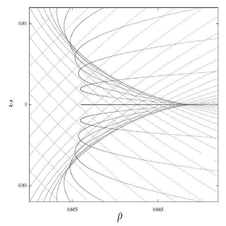
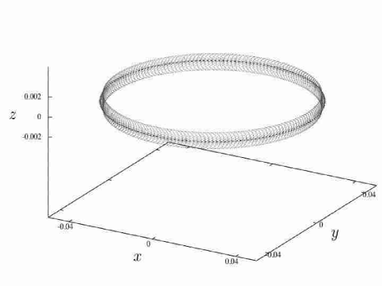
Figure 2: (a) Dark matter flows near the inner caustic for the initial velocity field $\vec{v}=-0.1\,\sin\theta\;\hat{\phi}$. The inner caustic is a ring whose cross section has three cusps, one of which points away from the galactic center. The three cusps are clearly visible in the figure. There are four flows everywhere inside the caustic surface, and two everywhere outside. (b) The axially symmetric tricusp ring in three dimensions. Note that here, and in many subsequent figures, the caustic is stretched in the $z$ direction for greater clarity.

In previous work sing , it was shown by analytical methods that the inner caustic is a tricusp ring when the initial velocity field $\vec{v}(\vec{r})$ of the infalling particles is dominated by net overall rotation. A tricusp ring is a closed tube whose cross section is a section of an elliptic umbilic catastrophe cat . We confirm this result in Section IV. Fig. 2 shows an axially symmetric tricusp ring as it appears in our simulations.

However, as will be shown below (Section III), the leading theory for the origin of the angular momentum of galaxies, namely tidal torque theory Pee ; Dor ; Whi , predicts that the initial velocity field of dark matter particles is a pure gradient. A pure gradient field is of course irrotational ($\vec{\nabla}\times\vec{v}=0$). It can nonetheless carry net angular momentum $\vec{L}=\int d^{3}r~{}\rho(\vec{r})~{}\vec{r}\times\vec{v}(\vec{r})$ because the density $\rho$ is inhomogeneous.

Motivated by tidal torque theory, we want to determine the structure of the inner caustics of galactic halos when the initial velocity field is irrotational and, more generally, when the initial velocity field is not dominated by net overall rotation. We address this issue by simulating the infall of cold collisionless particles in a fixed gravitational potential well. The inner caustic is revealed by finding the locus of points where the Jacobian of the map between the initial and final positions of the particles vanishes, i.e. where the map is singular.

We consider all initial velocity fields which are linear in position $\vec{r}$, i.e. fields of the type $\vec{v}=M\,\vec{r}$ where $M$ is a $3\times 3$ real matrix. We set $Tr(M)=0$ and more generally ignore the radial component $v_{r}=\hat{r}\cdot\vec{v}\,$ because it does not contribute to angular momentum and hence does not have much influence upon the inner caustics. Tidal torque theory predicts $M^{T}=M$, but we consider the more general case in which $M$ has both symmetric and anti-symmetric parts.

The outline of our paper is as follows. In Section II, we introduce the formalism of zero velocity dispersion flows and caustics, and give an existence proof of inner caustics. In Section III, we discuss our numerical techniques and the initial conditions expected from tidal torque theory. In Section IV, we simulate flows which are dominated by net overall rotation, confirm that the inner caustic is a tricusp ring in that case, and demonstrate the stability of the tricusp ring under small perturbations. In Section V we simulate flows which are not dominated by overall rotation and derive the structure of inner caustics for those cases. In Section VI, we summarize our conclusions.

In this paper, unless stated otherwise, the words “circle” and “sphere” will be used in their topological, rather than geometrical, sense. So an ellipse will be called a circle, etc.

II Existence proof of inner caustics

Consider a flow of cold collisionless particles falling from all directions in and out of the gravitational potential well of a galaxy. That the particles are collisionless means that they move under the influence of purely gravitational forces. We assume in this paper that Newtonian gravity applies, and so the particles obey the equation of motion

$${d^{2}\vec{r}\over dt^{2}}~{}=~{}-~{}\vec{\nabla}\Phi(\vec{r},t)$$ (1)

where $\Phi(\vec{r},t)$ is the gravitational potential of the galaxy. Note however that the existence proof of inner caustics given below would hold equally well in General Relativity. That the particles are cold means that they have negligible velocity dispersion. We set the velocity dispersion equal to zero. However, the presence of a small velocity dispersion does not affect the existence of caustics, and does not change their structure. It only cuts off the divergence of the dark matter density at the location of the caustics.

As was mentioned in the Introduction, CDM particles lie on a 3-dim. hypersurface in 6-dim. phase space. Because the number of particles is huge - of order $10^{84}$ axions and/or $10^{68}$ neutralinos per galactic halo - the particles can be labeled by three continuous parameters $\vec{\alpha}=(\alpha_{1},\alpha_{2},\alpha_{3})$ which are chosen arbitrarily. For example, one may choose $\vec{\alpha}$ to be the position $\vec{q}$ of the particle at some early initial time $t_{\rm in}$, before shell crossings have occurred. Other parametrizations may be more convenient however, depending on the problem at hand.

Let $\vec{x}(\vec{\alpha};t)$ be the position of the particle labeled $\vec{\alpha}$, at time $t$. After shell crossings have occurred, there will in general be particles with different values of $\vec{\alpha}$ at the same location $\vec{r}$. Let $\vec{\alpha}_{j}(\vec{r},t)$, with $j=1...n(\vec{r},t)$, be the solutions of $\vec{r}=\vec{x}(\vec{\alpha};t)$. Thus $n(\vec{r},t)$ is the number of distinct flows at location $\vec{r}$ at time $t$. $n$ is always a positive odd integer because $n=1$ to start with (before shell crossings have occurred) and the number of solutions of $\vec{r}=\vec{x}(\vec{\alpha};t)$ can only change by two at a time. Let ${d^{3}N\over d\alpha^{3}}(\vec{\alpha})$ be the number density of particles in the chosen parameter space. The mass density of particles in physical space is then sing

$$d(\vec{r},t)=m\sum_{j=1}^{n(\vec{r},t)}{d^{3}N\over d\alpha^{3}}(\vec{\alpha}){1\over|D(\vec{\alpha},t)|}~{}\bigg{|}_{\vec{\alpha}=\vec{\alpha}_{j}(\vec{r},t)}$$ (2)

where $m$ is the particle mass and

$$D(\vec{\alpha},t)=det\left({\partial\vec{x}(\vec{\alpha},t)\over\partial\vec{\alpha}}\right)~{}~{}~{}\ .$$ (3)

The magnitude of $D$ is the Jacobian of the map $\vec{\alpha}\rightarrow\vec{x}$. Caustics occur where $D=0$, i.e. where the map is singular. Note that, although $D$ is not reparametrization invariant, the density $d$ and the caustic condition $D=0$ are reparametrization invariant. Caustics lie generically on 2-dim. surfaces because, in general, the condition $D=0$ defines a surface in physical space. Only in special cases does the condition $D=0$ define an isolated line or point. Hence isolated line caustics and isolated point caustics are degenerate cases; they are unstable towards becoming caustic surfaces. Finally note that the map $\vec{\alpha}\rightarrow\vec{x}$ is singular where the number of flows $n$ changes. So caustics lie generically at the boundaries between regions which have different numbers of flows. On one side of a caustic surface are two more flows than on the other.

We now show that a continous flow of CDM particles falling in and out of a gravitational potential well cannot be free of caustics. Let us define a geometrical sphere of radius $R$ surrounding the potential well. The precise value of $R$ and the precise location of the sphere’s center do not matter. Let us label the particles by $\vec{\alpha}=(\theta,\phi,\tau)$ where $\tau$ is the time when the particle crosses the sphere on its way into the well, and $\theta$ and $\phi$ are the polar coordinates of its crossing point on the sphere. $\vec{x}(\theta,\phi,\tau;t)$ is the position of the particle as a function of time $t$. We will show that, at any $t$,

$$D=det~{}{\partial(x,y,z)\over\partial(\theta,\phi,\tau)}={\partial\vec{x}\over\partial\tau}\cdot\left({\partial\vec{x}\over\partial\phi}\times{\partial\vec{x}\over\partial\theta}\right)$$ (4)

vanishes at at least one point inside the sphere. The flow is considered at an arbitrary fixed time $t$. We will suppress the label $t$ henceforth.

For each $(\theta,\phi)$, the initial crossing time parameter $\tau$ has some range: $\tau_{\rm out}(\theta,\phi)<\tau<\tau_{\rm in}(\theta,\phi)$ where $\tau_{\rm in}~{}(\tau_{\rm out})$ is the initial crossing time of particles presently crossing the sphere on the way in (out). [The careful reader may notice that $\tau_{\rm in}(\theta,\phi)=t$, but this does not play a special role in what’s to follow.] Let us choose the origin $\vec{x}=0$ at the center of the sphere and consider the function of three variables $r(\theta,\phi,\tau)=\sqrt{\vec{x}(\theta,\phi,\tau)\cdot\vec{x}(\theta,\phi,\tau)}$. We have $~{}{\partial r\over\partial\tau}|_{\theta,\phi,\tau_{\rm out}(\theta,\phi)}~{}<~{}0~{}$ and $~{}{\partial r\over\partial\tau}|_{\theta,\phi,\tau_{\rm in}(\theta,\phi)}~{}>~{}0$. Hence for all $(\theta,\phi)$ there exists $\tau_{0}(\theta,\phi)$ such that

$$r(\theta,\phi,\tau_{0}(\theta,\phi))={\rm min}~{}r(\theta,\phi,\tau)\equiv r_{\rm min}(\theta,\phi)~{}~{}~{}\ ,$$ (5)

where the minimum is over $\tau\in[\tau_{\rm out}(\theta,\phi),\tau_{\rm in}(\theta,\phi)]$ for fixed $(\theta,\phi)$. $r_{\rm min}(\theta,\phi)$ is the closest distance to the origin among all particles labeled $(\theta,\phi)$. Let us first assume that $r_{\rm min}(\theta,\phi)\neq 0$ for some $(\theta,\phi)$ . We will return later to the opposite case, where $r_{\rm min}(\theta,\phi)=0$ for all $(\theta,\phi)$.

We have

$${\partial r\over\partial\tau}\bigg{|}_{\theta,\phi,\tau_{0}(\theta,\phi)}={\vec{x}\over r}\cdot{\partial\vec{x}\over\partial\tau}\bigg{|}_{\theta,\phi,\tau_{0}(\theta,\phi)}=0~{}~{}~{}\$$ (6)

for all $(\theta,\phi)$ such that $r_{\rm min}(\theta,\phi)\neq 0$. Now, $r_{\rm min}(\theta,\phi)$ has a maximum value over the sphere $S_{2}=\{(\theta,\phi)\}$. Let $(\theta_{0},\phi_{0})$ be such that

$$r_{\rm min}(\theta_{0},\phi_{0})={\rm max}~{}r_{\rm min}(\theta,\phi)~{}~{}~{}\ .$$ (7)

We have then

$${\partial r\over\partial\theta}\bigg{|}_{\vec{\alpha}_{0}}~{}=~{}{\vec{x}\over r}\cdot{\partial\vec{x}\over\partial\theta}\bigg{|}_{\vec{\alpha}_{0}}=0~{}~{},~{}~{}{\partial r\over\partial\phi}\bigg{|}_{\vec{\alpha}_{0}}~{}=~{}{\vec{x}\over r}\cdot{\partial\vec{x}\over\partial\phi}\bigg{|}_{\vec{\alpha}_{0}}=0$$ (8)

with $\vec{\alpha}_{0}\equiv(\theta_{0},\phi_{0},\tau_{0}(\theta_{0},\phi_{0}))$. Note that $\vec{x}_{0}\equiv\vec{x}(\vec{\alpha}_{0})\neq 0$. Eqs. (6) and (8) imply that ${\partial\vec{x}\over\partial\theta}|_{\vec{\alpha}_{0}}$, ${\partial\vec{x}\over\partial\phi}|_{\vec{\alpha}_{0}}$ and ${\partial\vec{x}\over\partial\tau}|_{\vec{\alpha}_{0}}$ are all perpendicular to $\vec{x}_{0}$. Hence those three vectors are linearly dependent, and therefore $D(\vec{\alpha}_{0})=0$. This implies that $\vec{x}_{0}$ is the location of a caustic. Note that $\vec{x}_{0}$ depends on the choice of origin. If we move the origin about, $\vec{x}_{0}$ will move too. Thus the inner caustic is in general spatially extended. This is as expected since caustics lie generically on surfaces.

Next we consider what happens in the special case where $r_{\rm min}(\theta,\phi)=0$ for all $(\theta,\phi)$. Then $\vec{x}(\theta,\phi,\tau_{0}(\theta,\phi))=0$ for all $(\theta,\phi)$. Therefore, for $\tau$ near $\tau_{0}(\theta,\phi)$,

$$\vec{x}(\theta,\phi,\tau)=\vec{\nu}(\theta,\phi)~{}(\tau-\tau_{0}(\theta,\phi))+O((\tau-\tau_{0}(\theta,\phi))^{2})$$ (9)

where $\vec{\nu}(\theta,\phi)={\partial\vec{x}\over\partial\tau}\bigg{|}_{\theta,\phi,\tau_{0}(\theta,\phi)}$. We may reparametrize $\theta^{\prime}=\theta,~{}\phi^{\prime}=\phi,~{}\tau^{\prime}=\tau-\tau_{0}(\theta,\phi)$, and rename $(\theta^{\prime},\phi^{\prime},\tau^{\prime})\rightarrow(\theta,\phi,\tau)$. In this parametrization, $\vec{x}(\theta,\phi,\tau)=\vec{\nu}(\theta,\phi)\tau+O(\tau^{2})$ for small $\tau$. Hence

$$D(\theta,\phi,\tau)=\vec{\nu}(\theta,\phi)\cdot\left({\partial\vec{\nu}\over\partial\theta}\times{\partial\vec{\nu}\over\partial\phi}\right)\tau^{2}~{}~{}~{}\ .$$ (10)

Since $D=0$ at $\tau=0$, the origin is the location of a caustic. This completes the proof. Note that the case $\vec{x}_{0}=0$ is special since the whole inner caustic has collapsed to a point.

To conclude this section, let us remark that in the situation discussed here, where CDM particles fall in and out of a gravitational potential well, the number of participating flows inside the sphere with radius $R$ is everywhere an even integer. Indeed just inside the $r=R$ surface there are two flows, one going in and one going out, and (as remarked earlier) the number of flows can only change by two at a time. The reader may wonder how this fits with the statement that the number of flows is everywhere odd. The resolution of this little puzzle is that, in actual realizations such as a galactic halo, there is always an odd number of additional flows present which are not participating in the in and out flow under consideration.

III Initial conditions and numerical techniques

In this section we describe how the simulations are done. A central issue is the initial conditions we give to the particles. In subsection A we show that in the tidal torque theory for the origin of the angular momentum of spiral galaxies the flow of CDM particles is irrotational to all orders in perturbation theory, i.e. to all orders in an expansion in powers of the density perturbations. In subsection B, we present the initial conditions used in the simulations. They are a generalization of the prediction of tidal torque theory to allow for rotational flow as well as irrotational flow. In subsection C, we describe the steps carried out in doing the simulations.

III.1 Irrotational flow in tidal torque theory

Net rotation is a striking property of isolated spiral galaxies. Yet it is not clear at present that the origin of this net rotation is well understood Pri . The leading hypothesis is that net rotation of spiral galaxies is the result of torque applied by the tidal gravitational forces of neighboring density perturbations in the very early stages of structure formation Pee ; Dor ; Whi . This hypothesis is called “tidal torque theory”. It is assumed in this context that general relativisitic effects are unimportant, and that Newtonian gravity applies.

In CDM cosmology, density perturbations enter the non-linear regime when shell crossings occur and caustics form. Before that time, or wherever shell crossings have not occurred yet, there is a single flow at every physical location $\vec{r}$. Let us call $\vec{v}(\vec{r},t)$ the velocity of that primordial flow. In the formalism of Section II, $\vec{v}(\vec{r},t)$ is obtained by eliminating $\vec{\alpha}$ from $\vec{r}=\vec{x}(\vec{\alpha},t)$ and $\vec{v}={\partial\vec{x}\over\partial t}(\vec{\alpha},t)$. For collisionless particles

$${d\vec{v}\over dt}(\vec{r},t)={\partial\vec{v}\over\partial t}(\vec{r},t)+(\vec{v}(\vec{r},t)\cdot\vec{\nabla})\vec{v}(\vec{r},t)=-\vec{\nabla}\Phi(\vec{r},t)$$ (11)

where $\Phi(\vec{r},t)$ is the gravitational potential. Eq. (11) neglects relativistic effects such as the gravitomagnetic force of General Relativity. Eq. (11) implies

$${\partial\over\partial t}(\vec{\nabla}\times\vec{v}) = -\vec{\nabla}\times[(\vec{v}\cdot\vec{\nabla})\vec{v}]$$ (12)

$$= -\hat{i}\epsilon_{ijk}[(\partial_{j}v_{l})(\partial_{l}v_{k})+v_{l}\partial_{l}\partial_{j}v_{k}]~{}~{}\ .$$

If $\vec{v}=\vec{\nabla}\chi$, both terms on the RHS of Eq. (12) vanish. Hence a pure gradient initial velocity field remains pure gradient at all times.

In zeroth order of perturbation theory, the flow is given by Hubble’s law: $\vec{v}(\vec{r},t)=H(t)\vec{r}$ where $H(t)={\dot{a}\over a}$ and $a(t)$ is the scale factor. That velocity field is certainly a pure gradient. In first order, the particle trajectories are given by Zel

$$\vec{x}(\vec{q},t)=a(t)[\vec{q}-b(t)\vec{\nabla}_{q}\Phi(\vec{q})]$$ (13)

where $\vec{q}$ is the particle’s position at a very early time, and $\Phi(\vec{q})$ is the gravitational potential. [The latter is time independent in first order perturbation theory when expressed in terms of the co-moving coordinate $\vec{q}$, i.e. $\Phi(\vec{r}=a(t)\vec{q},t)=\Phi(\vec{q})$.] In the matter dominated era, both $a(t)$ and $b(t)$ are proportional to $t^{2\over 3}$. As expected, the velocity field implied by Eq. (13) is irrotational. Our remark implies that the velocity field remains irrotational to all orders of perturbation theory.

III.2 The linear initial velocity field approximation

Eq. (13) implies

$$\vec{v}(\vec{r},t)=H(t)\vec{r}-a(t){db\over dt}(t)~{}\vec{\nabla}_{q}\Phi(\vec{q})|_{\vec{q}={1\over a(t)}\vec{r}}~{}~{}\ .$$ (14)

Following ref. Whi , let us choose $\vec{q}=0$ at a minimum of $\Phi$ and expand $\Phi$ in Taylor series up to second order in the $q$’s. The velocity field is then a linear function of position:

$$\vec{v}(\vec{r})=M~{}\vec{r}$$ (15)

where $M$ is a symmetric ($M^{\rm T}=M$) $3\times 3$ matrix. When a shell of particles surrounding a galaxy approaches turnaround, its initial Hubble expansion has been canceled by the attractive gravitational force of the galaxy. For such a shell the trace of $M$ is approximately zero.

In Sections IV and V we numerically integrate the equations of motion of particles falling in and out of the galactic gravitational potential well. The particles are given initial conditions on a geometrical turnaround sphere as follows. The particle labeled ($\theta,\phi,\tau$) starts at time $\tau$ at location

$$\vec{r}_{\rm in}(\theta,\phi)=R~{}\vec{n}(\theta,\phi)$$ (16)

where $\vec{n}(\theta,\phi)$ is the unit vector in the direction defined by polar angle $\theta$ and azimuth $\phi$. $R$ is the radius of the turnaround sphere. The particles are assigned velocities of the form of Eq. (15) with $Tr~{}M=0$. We write $M=S+A$ with $S^{\rm T}=S$ and $A^{\rm T}=-A$. Tidal torque theory predicts $A=0$. However, as tidal torque theory may not be the final word on the origin of the angular momentum of galaxies, we will study the inner caustics for $A\neq 0$ as well as $A=0$.

We believe the above set of initial conditions is sufficiently general for our purpose of studying the structure of inner caustics. Indeed, the structure of inner caustics is determined by the distribution of distances of closest approach of the particles falling in. This in turn is determined by the distribution of angular momenta on the turnaround sphere, or equivalently by the tangential components of the initial velocity field on the turnaround sphere. Caustics are stable under deformations. So to find the structure of inner caustics it is not necessary to use the most general initial conditions, but only initial conditions which are sufficiently representative of those that occur in reality. We expect that to include higher order terms in the Taylor expansion of the initial velocity field as a function of position will only deform, without changing their essential structure, the inner caustics found when assuming the initial velocity field is of the form of Eq. (15). We verify this expectation explicitly in the case of the tricusp caustic ring when we study its stability in Section IV.

We choose coordinate axes such that $S$ is diagonal:

$$M={1\over R}\left(\begin{array}[]{ccc}g_{1}&-c_{3}&c_{2}\\ c_{3}&g_{2}&-c_{1}\\ -c_{2}&c_{1}&-g_{1}-g_{2}\end{array}\right)~{}~{}~{}\ .$$ (17)

$g_{1}$ and $g_{2}$ parametrize the symmetric part of $M$ which yields the gradient part of $\vec{v}$, whereas $c_{1}$, $c_{2}$ and $c_{3}$ parametrize the anti-symmetric part of $M$ which yields the curl part of $\vec{v}$ and describes a rigid rotation of angular velocity $\vec{\omega}={\vec{c}\over R}$. In terms of the five parameters, the components of the initial velocity field tangent to the turnaround sphere are

$$v_{\phi}(\theta,\phi) = \vec{v}\cdot\hat{\phi}$$

$$= (g_{2}-g_{1})\sin\theta~{}\sin\phi~{}\cos\phi-\cos\theta(c_{1}\cos\phi+c_{2}\sin\phi)+c_{3}\sin\theta$$

$$v_{\theta}(\theta,\phi) = \vec{v}\cdot\hat{\theta}$$ (18)

$$= \sin\theta~{}\cos\theta~{}[g_{1}(1+\cos^{2}\phi)+g_{2}(1+\sin^{2}\phi)]-c_{1}\sin\phi+c_{2}\cos\phi~{}~{}~{}~{}\ .$$

The radial component $\vec{v}\cdot\hat{r}$ of the initial velocity field does not contribute to the angular momentum, and is set equal to zero. We verify in Section IV that the inclusion of radial initial velocities on the turnaround sphere has very little effect on the position of tricusp caustic rings, and no effect on their structure.

To conclude this subsection, we discuss the symmetry properties of our initial velocity field. Almost always we take the gravitational potential to be spherically symmetric, in which case the symmetry properties of the initial velocity field are those of the subsequent evolution as well. In the irrotational case ($c_{1}=c_{2}=c_{3}=0$), the initial velocity field is reflection symmetric about the $x=0$, $y=0$ and $z=0$ planes. Moreover it is axially symmetric when two of the three eigenvalues ($g_{1}$, $g_{2}$, and $g_{3}=-g_{1}-g_{2}$) are equal. Most often we will chose the axes such that $g_{1}\leq g_{2}\leq g_{3}$. The parameter space is then $g_{1}\leq 0$ and $g_{1}\leq g_{2}\leq-{1\over 2}g_{1}$. When $g_{1}=g_{2}$, the initial velocity field is axially symmetric about the $z$ axis. When $g_{2}=-{1\over 2}g_{1}$, it is symmetric about the $x$ axis.

In the case of pure rotation ($g_{1}=g_{2}=0$), we may choose axes such that $\vec{c}=c\hat{z}$. The initial velocity field is always axially symmetric in this case. When $g_{1}$, $g_{2}$, $c_{1}$, $c_{2}$ and $c_{3}$ are all different from zero, the initial velocity field has no symmetry. When axial symmetry about the $z$ axis is imposed, $c_{1}=c_{2}=0$ and $g_{1}=g_{2}$.

III.3 How the simulations are done

We simulate a single flow of zero velocity dispersion falling in and out of a time independent gravitational potential $\Phi(r)$, which is specified below. The initial conditions are Eqs. (16,18) plus $v_{r}=\vec{v}\cdot\hat{r}=0$. We solve the equation of motion, Eq. (1), numerically to obtain for all $(\theta,\phi)$ the trajectory $\vec{x}(\theta,\phi,\tau;t)$ of the particle which started at position $(\theta,\phi)$ on the turnaround sphere, at time $\tau$. Since neither the potential $\Phi$ nor the initial conditions are time-varying, the simulated flows are stationary, i.e. $\vec{x}(\theta,\phi,\tau;t)=\vec{x}(\theta,\phi,t-\tau)$. The simulation of non-stationary flows would be straightforward but considerably more memory intensive and time consuming, without being more revealing of the structure of inner caustics. The only change with respect to simulations of stationary flows would be that the caustics deform in a time dependent way. This would not teach us anything new about the structure of inner caustics.

From $\vec{x}(\theta,\phi,t^{\prime}=t-\tau)$ we calculate $D=det~{}\frac{\partial(x,y,z)}{\partial(\theta,\phi,t^{\prime})}$. We then plot the points where $D=0$. The set of these points is the inner caustic surface.

Unless stated otherwise, $\Phi$ is the gravitational potential produced by the matter density profile:

$$\rho(r)={v_{\rm rot}^{2}\over 4\pi G(r^{2}+a^{2})}~{}~{}~{}\ ,$$ (19)

which implies an asymptotically flat rotation curve with rotation velocity $v_{\rm rot}$. $a$ is the core radius. We will refer to the density profile of Eq. (19) as the “isothermal” profile although it is only an appoximation to an exact isothermal profile. The equation of motion is then

$$\frac{d^{2}\vec{r}}{dt^{2}}=-\frac{v_{\rm rot}^{2}}{r}\left[1-\frac{a}{r}\tan^{-1}\left(\frac{r}{a}\right)\right]\hat{r}~{}~{}~{}\ .$$ (20)

We use everywhere $R$, the radius of the turnaround sphere, as the unit of distance and $v_{\rm rot}$ as the unit of velocity. So our unit of time is ${R\over v_{\rm rot}}$, which is of order the infall time. The core radius $a$ is always set equal to 0.0285.

The five parameters $g_{1},~{}g_{2},~{}c_{1},~{}c_{2}$ and $c_{3}$, when expressed in units of $v_{\rm rot}$, are related to and of order the dimensionless angular momentum $j$ defined in STW . It was estimated in that paper that the average of $j$ over the turnaround sphere is approximately 0.2 in the case of the Milky Way. This sets the overall scale for the values of $g_{1}~{}...~{}c_{3}$ we are interested in and which are used in our simulations. Note that it is the relative values of these five parameters that determines the structure of inner caustics. The overall scale of the parameters merely determines the overall size of the inner caustics relative to $R$.

Since we simulate the infall of a single cold flow in a fixed potential, the particle resolution is not a critical issue. We chose a resolution of one particle per degree interval in $\theta$ and $\phi$, and a time step of $10^{-4}$.

IV The tricusp ring

It was found in ref. sing that the inner caustic is a “tricusp ring” when the initial velocity distribution is dominated by a rotational component. A “tricusp ring” is a closed tube whose cross section has the tricusp shape characteristic of the elliptic umbilic ($D_{-4}$) catastrophe. In this section, we perform simulations of flows with initial velocity fields dominated by a rotational component, show that the inner caustic is indeed a tricusp ring and that this structure is stable under perturbations.

IV.1 Axially symmetric case

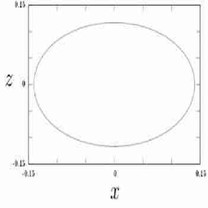
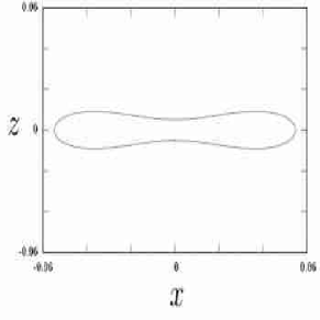
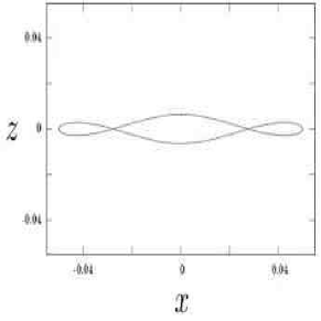
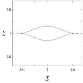
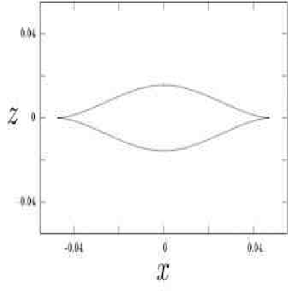
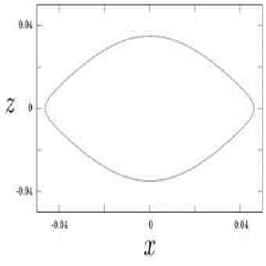
Figure 1: Infall of a cold collisionless shell for the axially symmetric initial velocity field $\vec{v}=-0.1\,\sin\theta\;\hat{\phi}$. The six frames show the shell in cross section at times $t^{\prime}$ = 1.206, 1.258, 1.263, 1.265, 1.267, 1.275. The continuous infall of many such shells produces the caustic shown in Figs. 2 and 2. $x$ and $z$ are in units of the outer turnaround radius $R$. Note that here, and in many subsequent figures, the $x$ and $z$ scales vary from frame to frame.

Consider the simple case where the initial velocity field is a linear function of the coordinates and is purely rotational, i.e. when Eq. (15) holds with an anti-symmetric matrix $M$. The initial velocity field is then axially symmetric. Let us choose coordinates such that $\vec{v}=c_{3}~{}\sin\theta~{}\hat{\phi}$. Fig. 1 shows the resulting infall of a single shell in $xz$ cross section, at successive times, for $c_{3}=-0.1$.

As the shell falls in, deviations from spherical symmetry appear due to the presence of angular momentum. The particles at the poles have zero angular momentum and fall in faster than the particles near the equator  [1]. They are the first to cross the $xy$ plane  [1]. The shell completes the process of turning itself inside out in Fig. 1, forming a crease. Finally the shell increases in size again and regains an approximately spherical shape [1].

The inner caustic occurs at and near the location of the crease in Fig. 1. Fig. 2 shows the flow near the crease in $\rho z$ cross section where $\rho\equiv\sqrt{x^{2}+y^{2}}$. The figure shows that the $\rho z$ plane is divided into two regions, one with two flows at each point and the other with four flows at each point. The boundary that separates these two regions is the caustic. The dark matter density is infinite there in the limit of zero velocity dispersion. Fig. 2 shows the caustic in three dimensions. It is indeed the “tricusp ring” described in ref. sing .

IV.2 Perturbing the initial velocity field

IV.2.1 Breaking axial symmetry

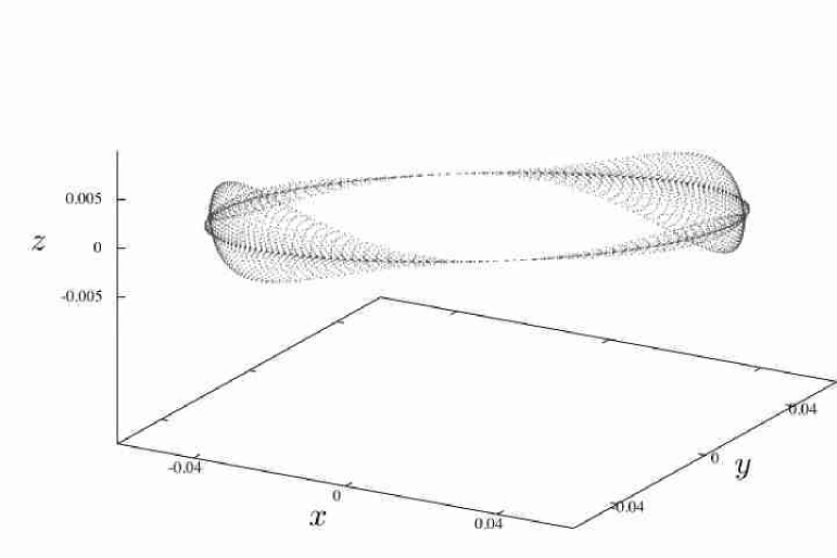
Figure 3: Tricusp ring for the initial velocity field of Eq. (18) with $c_{3}=-0.1,~{}g_{1}=-0.033,~{}g_{2}=0.0267$. It has reflection symmetry about the $xy$, $xz$ and $yz$ planes.

We introduce departures from axial symmetry by adding gradient terms, proportional to $g_{1}$ and $g_{2}$. Fig. 3 shows the inner caustic for the initial velocity field of Eqs. (18) with $c_{3}=-0.1,~{}g_{1}=-0.033,~{}g_{2}=0.0267$. It is again a tricusp ring but the cross section is now $\phi$-dependent. The tricusp shrinks to a point four times along the ring. In the neighborhood of each such point, the catastrophe is the full elliptic umbilic$(D_{-4})$ cat .

IV.2.2 A random perturbation

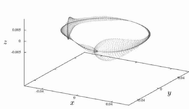
Figure 4: Tricusp ring for the initial velocity field given in Eq. (21).

We added randomly chosen perturbations to the previously discussed axially symmetric initial velocity field. The inner caustic shown in Fig. 4 is for the initial velocity field

$$\vec{v} = -0.1~{}\sin\theta~{}\hat{\phi}$$ (21)

$$- 0.01~{}\sin\theta~{}\left[\sin(2\phi)+0.5\sin(3\phi)+0.25\sin(4\phi)\right]\hat{\phi}$$

Although the caustic is deformed from what it was in Fig. 2, its structure remains a ring whose cross section is everywhere a tricusp.

IV.2.3 The effect of radial velocities

We added radial velocities to the previously discussed axially symmetric initial velocity field. We find that the radial velocity components result in only relatively small changes in the dimensions of the tricusp ring. For the initial velocity field

$$\vec{v}=c_{3}~{}\sin\theta~{}(\hat{\phi}+\hat{r})$$ (22)

with $c_{3}=-0.1$, the tricusp ring radius was decreased by 0.28%, compared to what it was for the original initial velocity field ($\vec{v}=c_{3}~{}\sin\theta~{}\hat{\phi}$), and the transverse dimensions of the tricusp ring were reduced by 11% and 14% in the directions perpendicular and parallel to the plane of the ring. For $c_{3}=-0.3$, the radius was reduced by 1.7% and the transverse dimensions by 69% and 73% respectively.

Let us explain why radial velocities on the turnaround sphere have only a small effect on the inner caustics. The inner caustics are determined by the distribution of distances $r_{\rm min}$ of closest approach to the galactic center of the infalling particles. The distance of closest approach is determined by angular momentum conservation: $\ell=r_{\rm min}v_{\rm max}$, where $\ell$ is specific angular momentum and $v_{\rm max}$ is the speed at the moment of closest approach. The latter is determined by energy conservation

$${1\over 2}v_{\rm max}^{2}={1\over 2}(v_{\phi}^{2}+v_{\theta}^{2}+v_{r}^{2})+\Phi(R)-\Phi(r_{\rm min})~{}~{}~{}\ .$$ (23)

The main contribution to $v_{\rm max}$ is from the gravitational potential energy released while the particle falls in. The initial velocity components provide only corrections to $v_{\rm max}$ which are second order in $v_{\phi},v_{\theta}$ and $v_{r}$. Since $\ell$ does not depend on $v_{r}$ at all, radial velocities produce only second order corrections to the distances of closest approach.

IV.3 Modifying the gravitational potential

In this subsection we verify that, when the initial velocity field is dominated by a rotational component, the inner caustic is a tricusp ring independently of the choice of gravitational potential.

IV.3.1 The NFW density profile

We carried out simulations of the infall of collisionless particles in the gravitational potential produced by the density profile of Navarro, Frenk and White nfw :

$$\rho(r)=\frac{\rho_{s}}{\frac{r}{r_{s}}{\left[1+\frac{r}{r_{s}}\right]}^{2}}~{}~{}~{}\ .$$ (24)

The scale length $r_{s}$ was chosen to be 25 kpc. $\rho_{s}$ was determined by requiring that the rotational velocity at galactocentric distance $r_{\odot}$ = 8.5 kpc is 220 km/s. The acceleration of a particle orbiting in the potential produced by the NFW density profile is then:

$$\vec{a}(r)=-\frac{(220~{}{\rm km/s})^{2}\;x^{2}_{\odot}}{r_{\odot}\;x^{2}}\left[\frac{\ln(1+x)-\frac{x}{1+x}}{\ln(1+x_{\odot})-\frac{x_{\odot}}{1+x_{\odot}}}\right]\;\hat{r}$$ (25)

where $x=r/r_{s}$ and $x_{\odot}=r_{\odot}/r_{s}$.

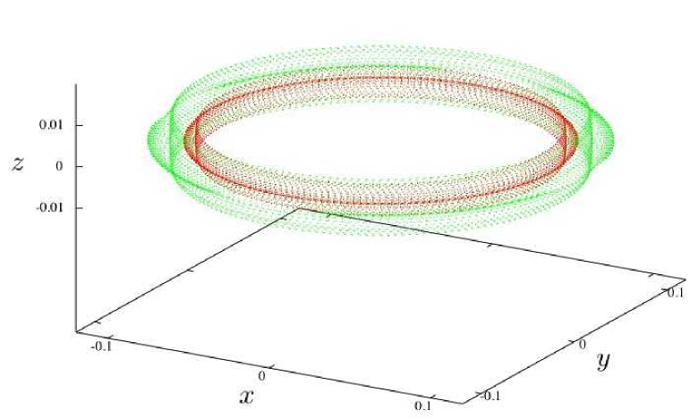
Figure 5: Tricusp rings caused by the same initial velocity field but different gravitational potentials. The larger ring (green) was obtained using the NFW profile, Eq. (24), while the smaller ring (red) was obtained using the density profile of Eq. (19).

Fig. 5 shows the result of two simulations plotted on the same figure. The outer caustic ring is obtained using the density profile of Eq. (24), while the inner caustic ring is obtained using the density profile of Eq. (19) with $v_{\rm rot}=220$ km/s and $a=4.96$ kpc. In both cases, the turnaround radius $R=174$ kpc and the initial velocity field $\vec{v}=0.2~{}\sin\theta~{}\hat{\phi}$. As always, the coordinates $x,y,z$ are in units of $R$. The inner caustic is a tricusp ring in each case, but with different dimensions. The ring caustic produced by the NFW profile has larger radius than that produced by the isothermal profile because the NFW gravitational potential is shallower than the isothermal one at the location of the caustic ($r_{\rm caustic}\simeq 16$ kpc). Since $\ell=r_{\rm min}~{}v_{\rm max}$ is the same, $r_{\rm min}$ is larger in the NFW case because $v_{\rm max}$ is smaller.

IV.3.2 Breaking spherical symmetry

We also simulated the infall of collisionless particles in a non spherically symmetric gravitational potential. For the latter, we chose the triaxial form:

$$\Phi(r)=-v_{\rm rot}^{2}\ln\left(\frac{R}{\sqrt{{\left(\frac{x}{a_{1}}\right)}^{2}+{\left(\frac{y}{a_{2}}\right)}^{2}+{\left(\frac{z}{a_{3}}\right)}^{2}}}\right)$$ (26)

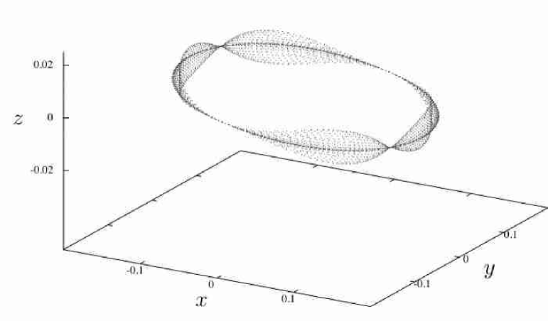
Figure 6: Tricusp ring for the initial velocity field $\vec{v}=0.2~{}\sin\theta~{}\hat{\phi}$ and the non spherically symmetric gravitational potential of Eq. (26).

where $a_{1}$, $a_{2}$ and $a_{3}$ are dimensionless numbers. Fig. 6 shows the inner caustic for the case where $a_{1}=0.95$, $a_{2}=1.0$ and $a_{3}=1.05$, and the initial velocity field $\vec{v}=0.2~{}\sin\theta~{}\hat{\phi}$. It is again a tricusp ring. Its axial symmetry is lost due to the absence of axial symmetry in the potential. The tricusp ring still has reflection symmetry about the $xy$, $yz$ and $xz$ planes. As in Fig. 3 the tricusp shrinks to a point four times along the ring.

V General structure of inner caustics

In this section, we describe the structure of inner caustics when the initial velocity field is not dominated by a rotational component. In subsection A, we discuss the axially symmetric case, whereas the non axially symmetric case is discussed in subsection B. In each subsection, we simulate first irrotational (i.e. pure gradient) initial velocity fields. As was mentioned in Section III, irrotational initial velocity fields are predicted by tidal torque theory. We will find the inner caustics produced by irrotational velocity fields to have a definite structure which we refer to as the “tent caustic”. After describing the tent caustic, we add a rotational component to the initial velocity field and see how the tent caustic deforms into a tricusp ring.

V.1 The axially symmetric case

The initial velocity field of Eqs. (18) is symmetric about the $z$ axis when $c_{1}=c_{2}=0$ and $g_{1}=g_{2}$. Then

$$\vec{v}={3\over 2}~{}g_{1}~{}\sin(2\theta)~{}\hat{\theta}+c_{3}~{}\sin\theta~{}\hat{\phi}~{}~{}~{}\ .$$ (27)

We first simulate the flow and obtain the inner caustic in the irrotational case, $c_{3}=0$. Next we see how the flow and inner caustic are modified when $c_{3}\neq 0$.

V.1.1 Infall of a cold collisionless shell

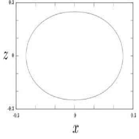
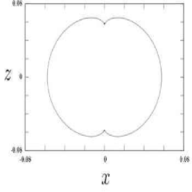
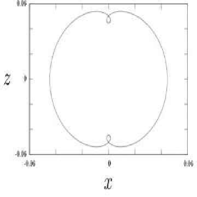
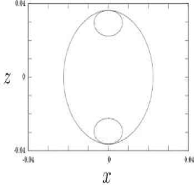
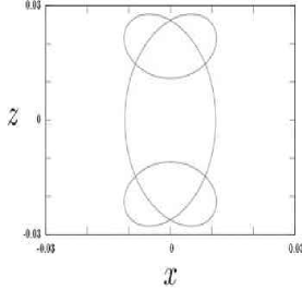
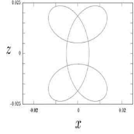
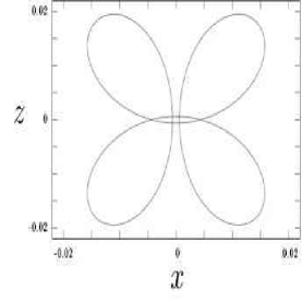
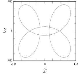
Figure 7: Infall of a cold collisionless shell for the axially symmetric initial velocity field $\vec{v}=-0.05~{}\sin(2\theta)~{}\hat{\theta}$. The shell is shown in $xz$ cross section at times $t^{\prime}$ = 1.132, 1.235, 1.241, 1.251, 1.256, 1.258, 1.260 and 1.261. The further time evolution is shown in Fig. 8. The continuous infall of many such shells produces the caustic shown in Fig. 10(a).

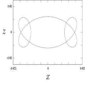
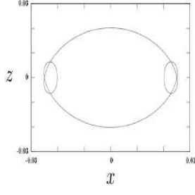
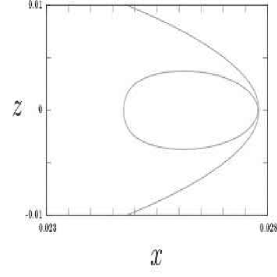
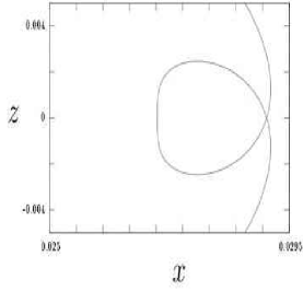
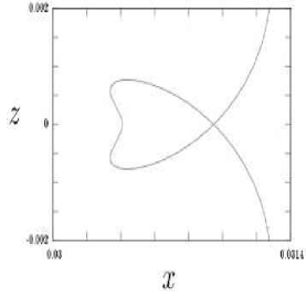
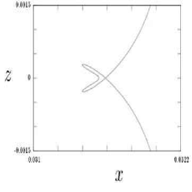
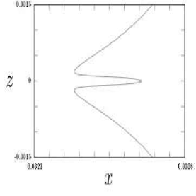
Figure 8: Continuation of the sequence of Fig. 7. The shell is shown at times $t^{\prime}$ = 1.265, 1.269, 1.271, 1.272, 1.273, 1.2737, 1.2742 and 1.280.

Figs. 7 and 8 show the infall of a cold collisionless shell whose initial velocity field is given by Eq. (27) with $c_{3}=0$ and $g_{1}=-0.0333$. Since $c_{3}=0$, each particle stays in the plane containing the $z$ axis and its initial position on the turnaround sphere. Figs. 7 and 8 show the particles in the $y=0$ plane. The angular momentum vanishes at $\theta=0$ and $\theta=\pi/2$ where $\theta$ is the polar coordinate of the particle at its initial position. Hence, the particles labeled $\theta=0$ and $\theta=\pi/2$ follow radial orbits. The angular momentum increases in magnitude from $\theta=\pi/2$, reaches a maximum at $\theta=\pi/4$ and returns to zero at $\theta=0$. The sign of the angular momentum does not change during this interval.

The shell starts out as shown in Fig. 7. As the shell falls in, the particles at $\theta\neq 0,\pi/2$ move towards the poles. These particles feel an angular momentum barrier and fall in more slowly than the particles at $\theta=0$. This results in the formation of a loop in Fig. 7. The formation of the loop implies a cusp caustic on the $z$ axis. The particles labeled $\theta=0$ and $\theta=\pi$ have crossed the $z=0$ plane and the particles labeled $\theta=\pi/2$ have crossed the $x=0$ plane in Fig. 7. The shell then takes the form shown in Fig. 7. The further evolution is shown in Fig. 8. The loop that is present near the $z=0$ plane in Fig. 8 disappears through the sequence of Figs. 8 - 8. The disappearance of the loop implies the existence of a cusp caustic in the $z=0$ plane as well. In Fig. 8 the shell has regained an approximately spherical form and is expanding to its original size.

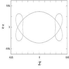
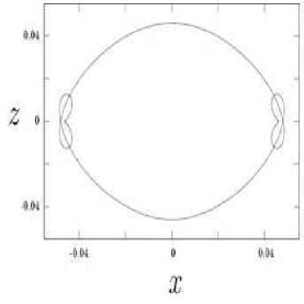
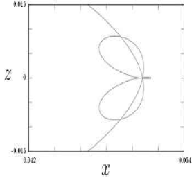
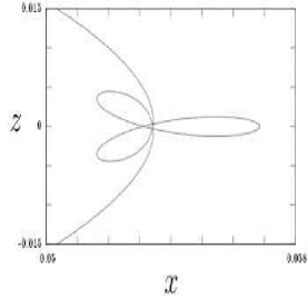
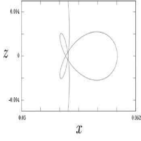
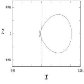
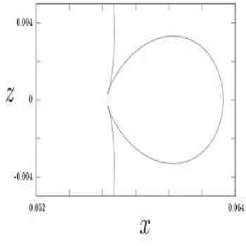
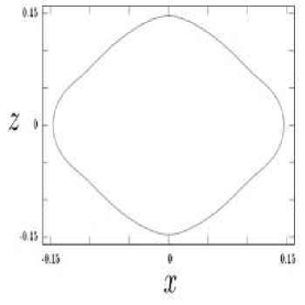
Figure 9: Same as Fig. 8 but for the initial velocity field $\vec{v}=-0.1~{}\sin(2\theta)~{}\hat{\theta}$. The shell is shown at times $t^{\prime}$ = 1.273, 1.280, 1.283, 1.285, 1.287, 1.2875, 1.2880 and 1.329. The earlier evolution is qualitatively the same as in Fig. 7. The continuous infall of many shells with this initial velocity field produces the caustic shown in Fig. 11(a).

For larger values of $|g_{1}|$ the early evolution is qualitatively the same as in Fig. 7, but the late evolution is qualitatively different from Fig. 8. Fig. 9 shows the late evolution of a cold collisionless shell with the initial velocity field of Eq. (27) with $c_{3}=0$ and $g_{1}=-0.0667$. The loop which is present near the $z=0$ plane in Fig. 9 disappears by a more complicated sequence [9 - 9] than was the case in Fig. 8. In Fig. 9 the particles near $\theta=\pi/2$ cross the $z=0$ plane before the sphere turns itself inside out. This crossover produces additional structure, and a more complicated caustic, than for the $g_{1}=-0.0333$ case. The critical value of $|g_{1}|$, below which the qualitative evolution is that of Fig. 8, and above which that of Fig. 9, is $g_{1*}\simeq 0.05$.

V.1.2 Caustic Structure

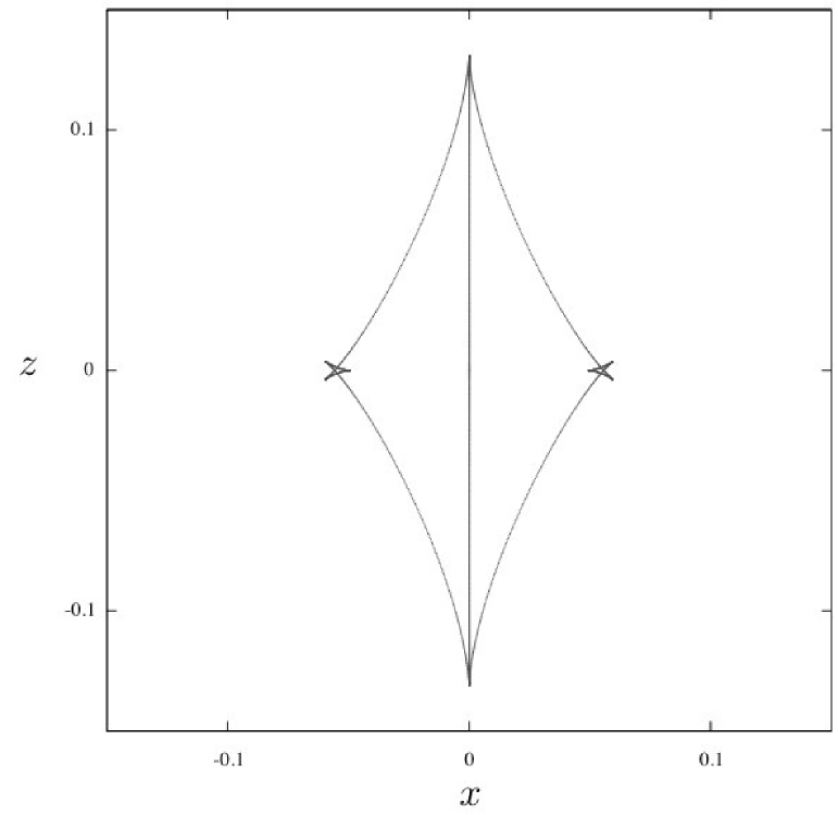
(a) Caustic structure.

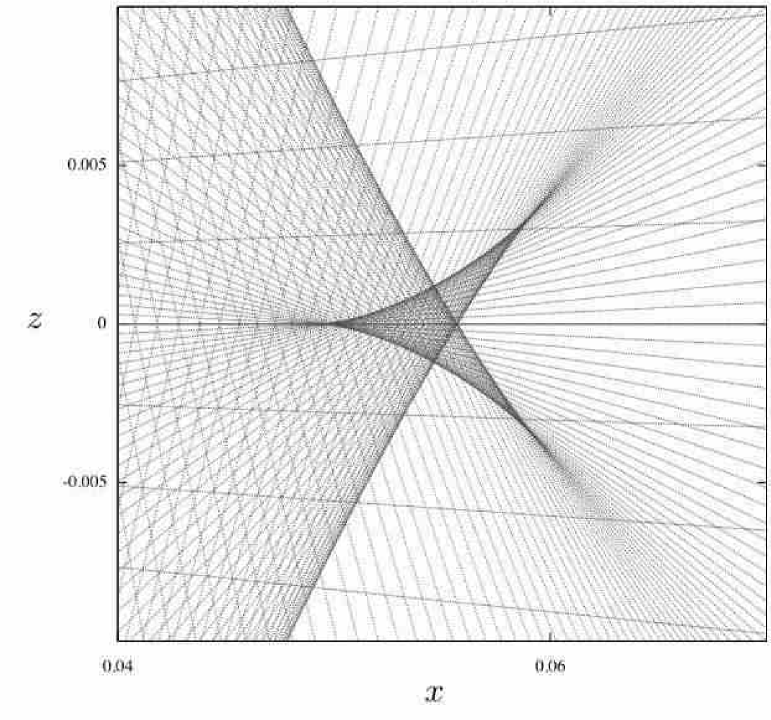
(b) Dark matter flows near the butterfly caustic.

Figure 11: Cross section of the inner caustic produced by the irrotational axially symmetric velocity field $\vec{v}=-0.1\sin\,2\theta\;\hat{\theta}$.

The inner caustic is a surface of revolution whose cross section is shown in Fig. 10(a) for the case $(c_{3},g_{1})=(0,-0.0333)$ and in Fig. 11(a) for $(c_{3},g_{1})=(0,-0.0667)$. For the sake of brevity, we call this structure a “tent caustic”. On the $z$ axis, there is a caustic line which we call the “tent pole”. The remainder of the caustic is called the “tent roof”. As was mentioned in Section II, caustic lines are not generic. The tent pole is a line in Figs. 10(a) and 11(a) only because the initial velocity field is axially symmetric and irrotational. We will see below that when axial symmetry is broken or when a rotational component is added, the tent pole becomes a caustic tube of a specific sort.

For $|g_{1}|<g_{1*}$ there is a cusp in the tent roof where it meets the $z=0$ plane and two cusps where the tent roof meets the tent pole, one at the top and one at the bottom. For $g_{1}<-g_{1*}$ the cusp in the $z=0$ plane is replaced by a butterfly catastrophe cat . The butterfly has three cusps and three points of self-intersection. The cusp in the $z=0$ plane transforms into a butterfly by increasing $|g_{1}|$. The latter parameter may therefore be called the “butterfly factor” Saunders .

If $g_{1}$ is chosen positive instead of negative, the behavior at the poles and the equator is reversed [see Eq. (27)] and we have cusps on the $x$ axis and either cusp or butterfly catastrophes on the $z$ axis, depending on the magnitude of $g_{1}$.

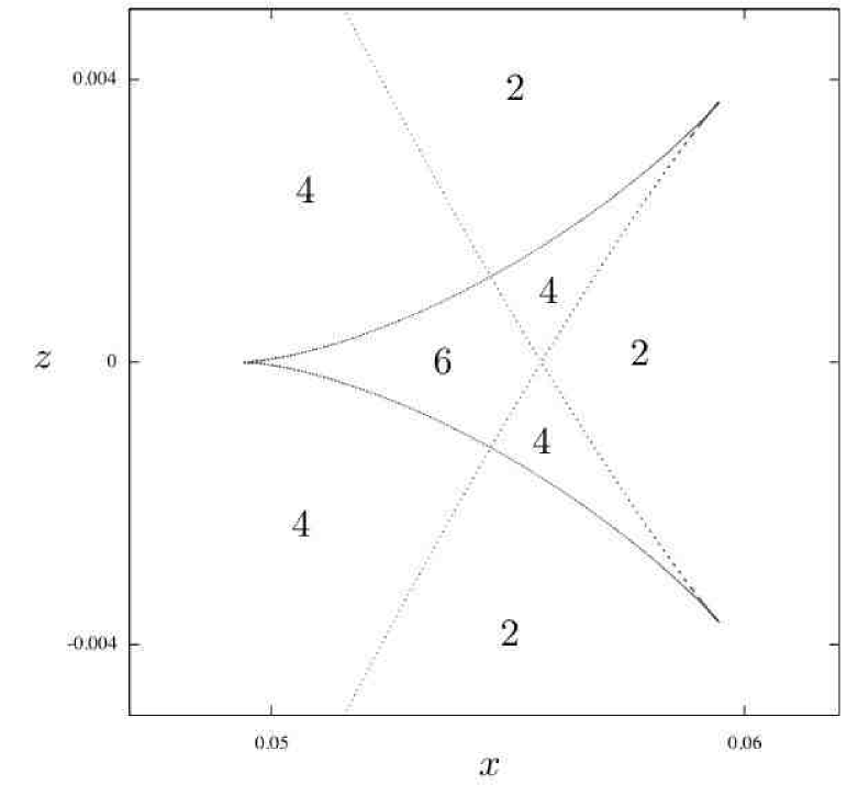
Figure 12: The butterfly catastrophe has three cusps, and three points where the caustic intersects itself. The number of flows in each region is indicated.

Fig. 10(b) shows the dark matter flows in the vicinity of the caustic for $|g_{1}|<g_{1*}$. There are four flows everywhere inside the caustic tent and two flows everywhere outside. Fig. 11(b) shows the dark matter flows in the vicinity of the butterfly caustic, for $g_{1}<-g_{1*}$. Fig. 12 shows the number of flows in each region of the butterfly caustic.

V.1.3 Adding a rotational component

Here we show, in the axially symmetric case, the effect of adding a rotational component to the initial velocity field. On the basis of the discussion in Section IV, we expect the tent caustic to transform into a tricusp ring. Fig. 13 shows the transformation. We start with an irrotational velocity field $(c_{3}=0)$ in 13 and increase $c_{3}$ until the rotational component dominates the velocity field, in 13. The tent pole on the $z$ axis, which is a line caustic in the irrotational case, changes to a tube of circular cross section. The radius of this tube increases until the tent caustic becomes indistinguishable from a tricusp ring.

V.2 Non axially symmetric case

We start off by discussing the flows and caustics resulting from irrotational initial velocity fields. With $\vec{c}=0$, Eqs. (18) become

$$\vec{v}=\xi~{}\sin\theta~{}\sin(2\phi)~{}\hat{\phi}+\sin(2\theta)(\xi~{}\sin^{2}\phi+g)~{}\hat{\theta}~{}~{}~{},$$ (28)

where $\xi\equiv{1\over 2}(g_{2}-g_{1})$ and $g\equiv g_{1}+{1\over 2}g_{2}$. $\xi$ is a measure of $\hat{z}$ axial symmetry breaking in the irrotational case. We first let $\xi\ll g$. Next, we explore all of $(g_{1},g_{2})$ parameter space. Finally, we add a rotational component by letting $c_{3}\neq 0$.

V.2.1 Irrotational, non axially symmetric perturbations

We saw in subsection V-A that there is a caustic line on the $z$ axis (the tent pole) when the initial velocity field is irrotational and axially symmetric. Fig. 14 shows the trajectories of the particles in the $z=0$ plane for such a case. The orbits are radial. Indeed all particles have zero angular momentum with respect to the $z$ axis when the initial velocity field is irrotational and axially symmetric. Because all trajectories intersect the $z$ axis, there is a pile up of particles on that axis and hence a caustic line.

Fig. 14 shows the trajectories of the particles in the $z=0$ plane for the initial velocity field of Eq. (28) with $\xi=0.01$ and $g=-0.05$. The particles do have angular momentum with respect to the $z$ axis now. The caustic line on the $z$ axis spreads onto a tube whose cross section is the diamond shaped envelope of particle trajectories shown in Fig. 14. That envelope has four cusps. The flows and caustic have reflection symmetry about the $xy$, $xz$ and $yz$ planes because the initial velocity field has those symmetries. Fig. 14 shows four flows inside the diamond-shaped caustic and two flows outside. The infall of dark matter particles from regions above and below the $z=0$ plane will add two more flows at each point, which are not shown in Fig. 14 for clarity.

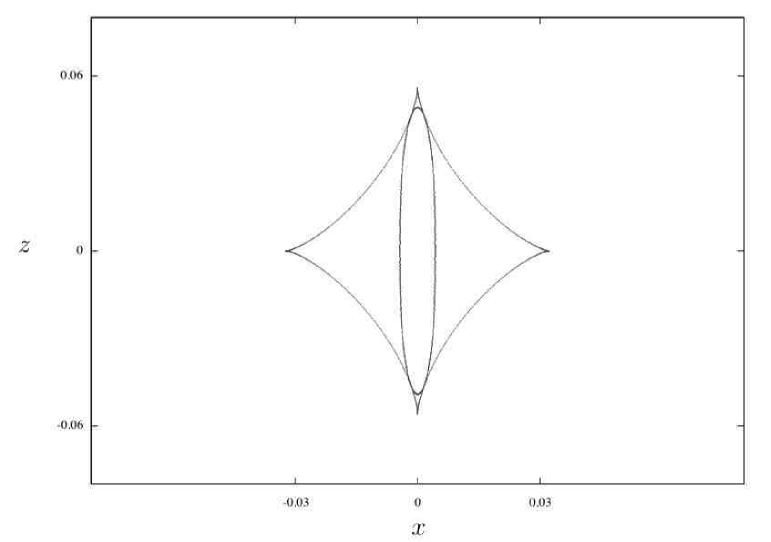
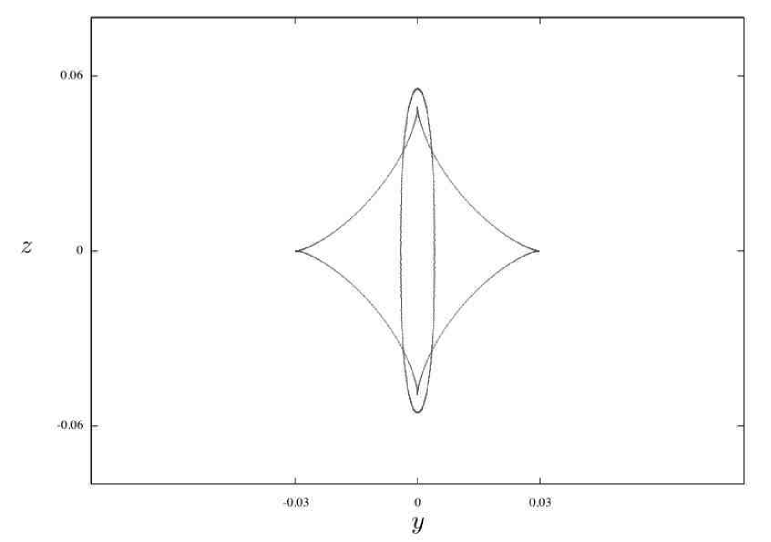
Figure 16: The tent caustic of Fig. 15 in (a) $y=0$ cross section and (b) $x=0$ cross section. The manner in which the tent pole is connected to the tent roof is described in detail in Fig. 17.

Fig. 15 shows the inner caustic in 3 dimensions for the initial velocity field of Eq. (28) with $\xi=0.005$ and $g=-0.05$. The tent pole has spread onto a tube with diamond shaped cross section, as in Fig. 14. Fig. 15 shows a succession of constant $z$ sections. The (topological) circles, which are sections of the tent roof, and the diamond structure can be seen clearly. Near the $z=0$ plane, there are six flows inside the diamond, four flows in the other regions inside the caustic tent, and two outside the tent. Fig. 16 shows $y=0$ and $x=0$ sections of the tent caustic.

V.2.2 A hyperbolic umbilic catastrophe

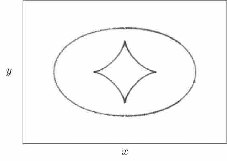
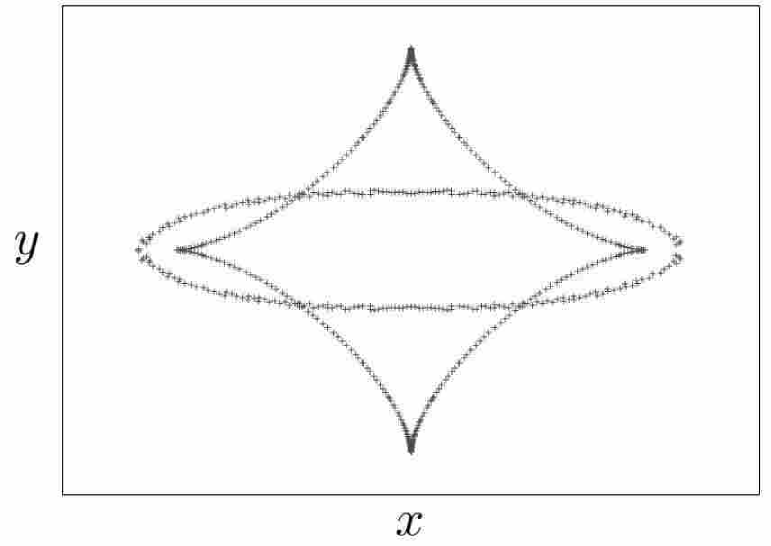
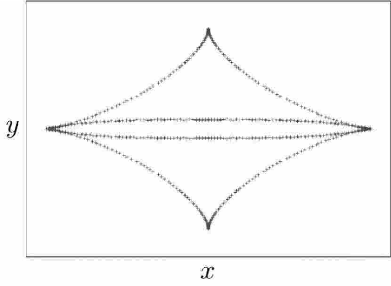
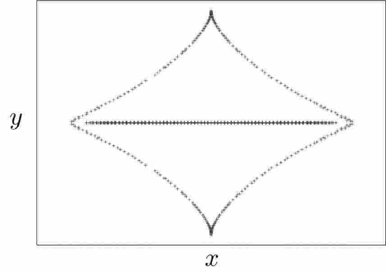
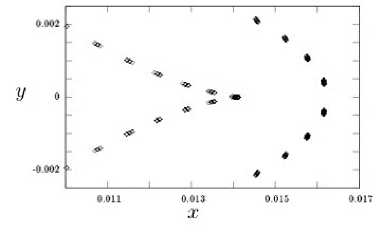
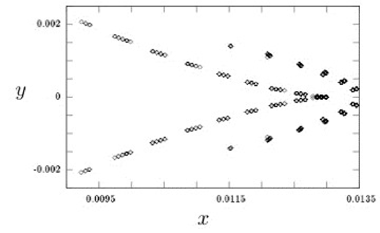
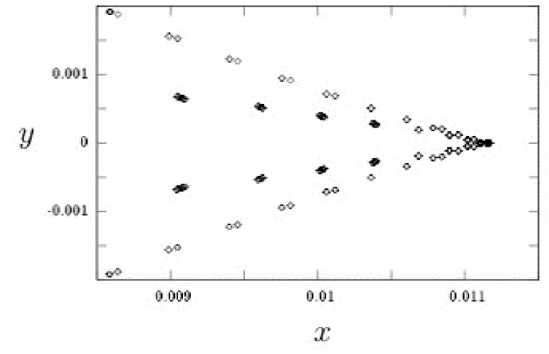
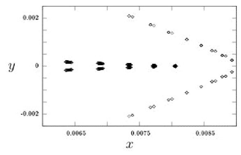
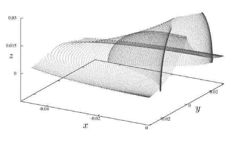
Figure 17: (a)-(d) Constant $z$ sections of the tent caustic of Fig. 15 in the region where the tent pole connects with the tent roof. In (a) the pole is entirely inside the roof. In (b) the cusps of the pole which are in the $x=0$ plane have pierced the roof. From (b) to (d) the parts of the pole and the roof near the $y=0$ plane traverse each other by forming hyperbolic umbilic catastrophes, one on the $x>0$ side and one on the $x<0$ side. (e)-(h) Constant $z$ sections of the tent caustic near the hyperbolic umbilic on the $x>0$ side, for greater detail. (i) the hyperbolic umbilic at $z>0,x<0$ in three dimensions.

Let us look more closely at the two regions (top and bottom) in Fig. 16 where the tent pole reaches and traverses the tent roof. Figs. 17 -  17 show $z$ = constant sections of the inner caustic in such a region. As $|z|$ is increased, the two cusps of the pole which are in the $x=0$ plane simply pierce through the roof, whereas the parts of the pole near the $y=0$ plane traverse the roof by forming with the latter two hyperbolic umbilic ($D_{+4}$) catastrophes cat , one on the positive $x$ side and one on the negative $x$ side. The sequence through which this happens is shown in greater detail in Figs. 17 -  17 for the hyperbolic umbilic on the positive $x$ side. The arc (section of the tent roof) and the cusp (section of the tent pole) approach each other until they overlap [17], forming a corner. After they have crossed, the roof section is cuspy whereas the pole section is smooth. The cusp is transferred from the tent pole to the tent roof as the two surfaces pass through one another. This behaviour is characteristic of the hyperbolic umbilic catastrophe. There are four hyperbolic umbilics embedded in the caustic tent structure, two ($x>0$ and $x<0$) at the top ($z>0$) and two at the bottom ($z<0$). The hyperbolic umbilic at $z>0$ and $x<0$ is shown in three dimensions in Fig. 17.

Let’s mention that the particles forming the pole and roof where they intersect in the $x=0$ plane originate from different patches of the initial turnarround sphere whereas the particles forming the pole and roof near a hyperbolic umbilic originate from the same patch of the initial turnaround sphere.

V.2.3 The $(g_{1},g_{2})$ landscape

Here we describe the inner caustic in the irrotational case for $g_{1}$ and $g_{2}$ far from those values where the flow is axially symmetric. Recall that the flow is symmetric about the $z$ axis when $g_{1}=g_{2}$ ($g_{3}=-2g_{1}$), about the $y$ axis when $g_{2}=-2g_{1}$ ($g_{3}=g_{1}$), and about the $x$ axis when $g_{2}=-{1\over 2}g_{1}$ ($g_{3}=g_{2}$). In terms of $\xi$ and $g$, these conditions for axial symmetry are $\xi=0$, $g=0$, and $\xi=-g$, respectively.

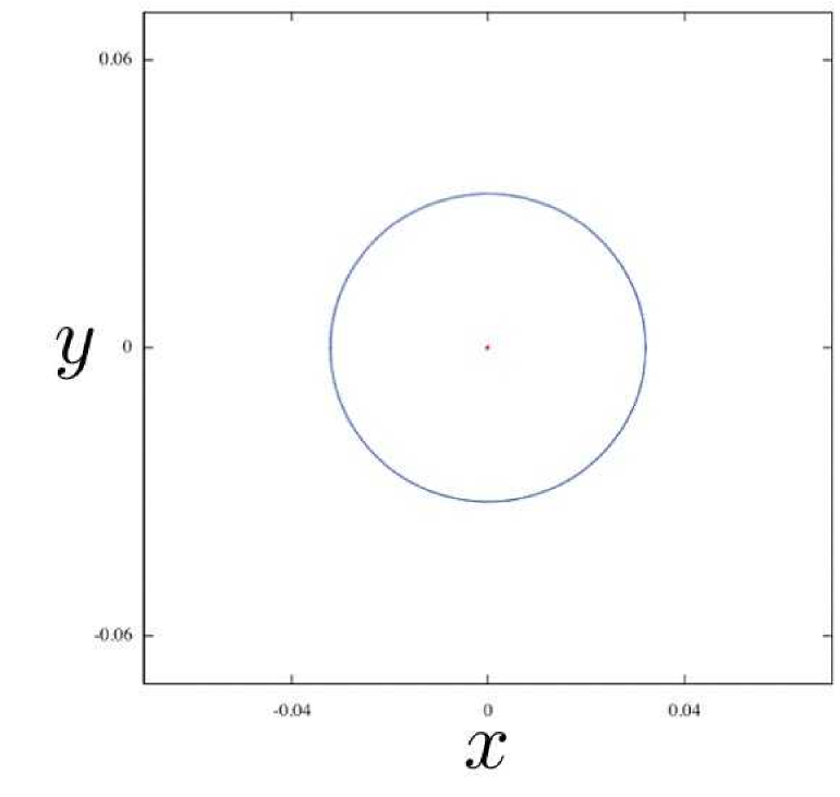
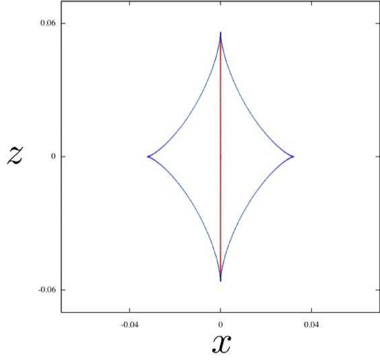
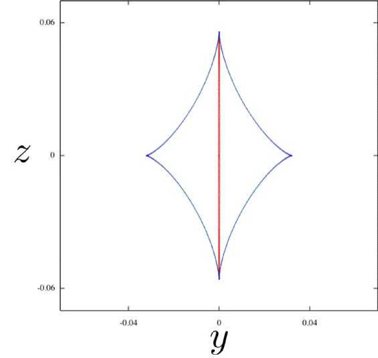
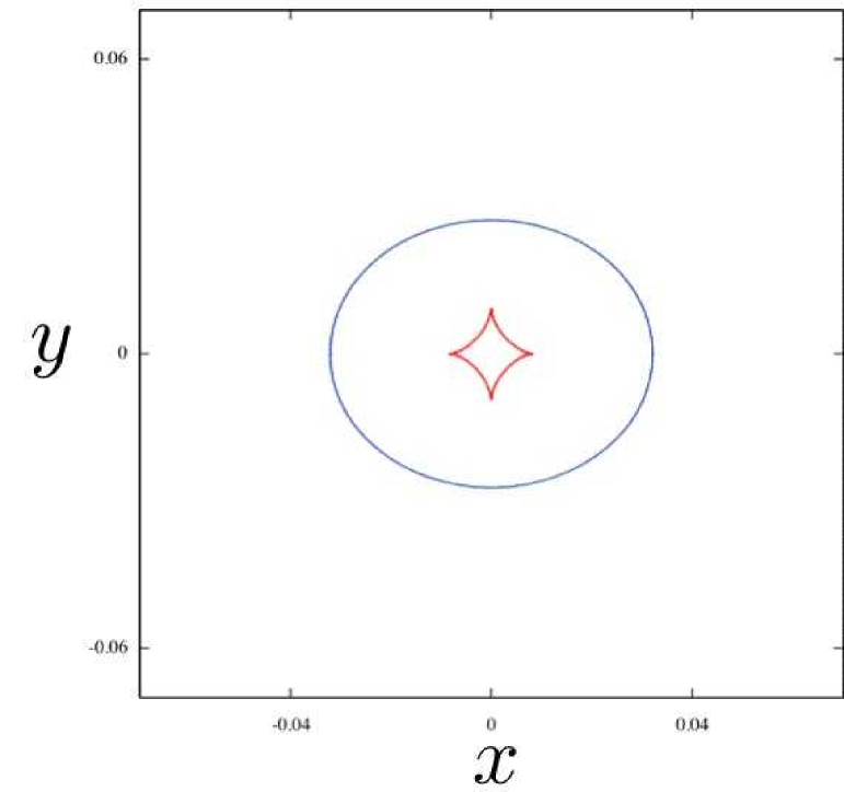
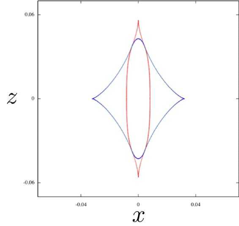
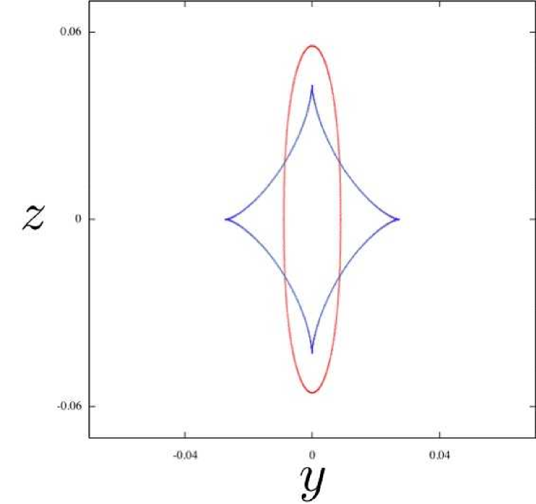
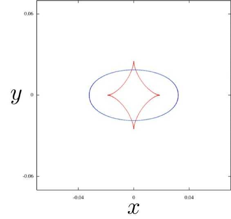
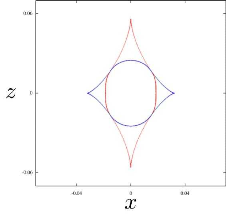
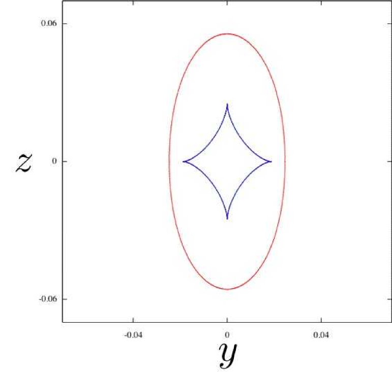
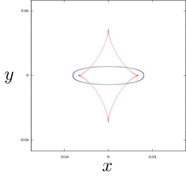
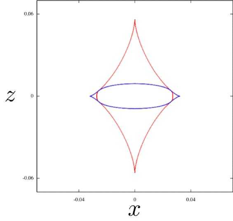
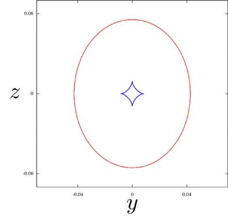
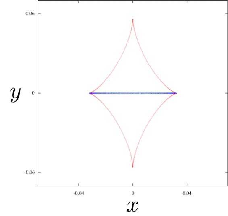
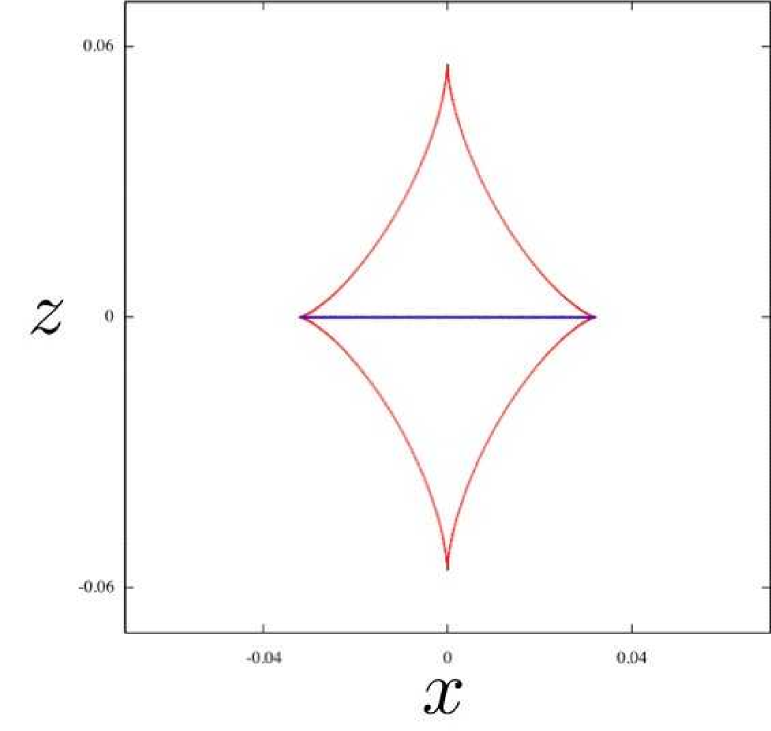
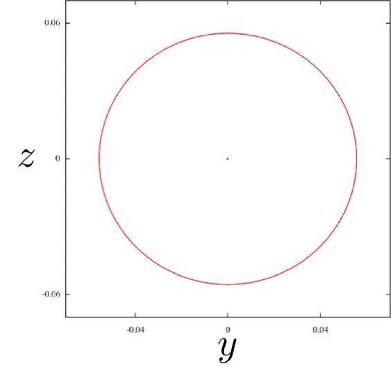
Figure 18: The first, second and third columns show respectively the $z=0$, $y=0$ and $x=0$ cross sections of the inner caustics produced by the irrotational initial velocity field of Eq. (28) for $(g_{1},g_{2})$ = (-0.033, -0.033), (-0.04,-0.02), (-0.05, 0), (-0.06, 0.02) and (- 0.067, 0.033) in five rows from top to bottom. During this sequence, the caustic transforms from a tent symmetric about the $z$ axis (first row) to a tent symmetric about the $x$ axis (last row). The roof of the caustic in the first row becomes the pole of the caustic in the last row (blue) and vice-versa (red).

The first, second and third column of Fig. 18 show respecively the $z=0$, $y=0$ and $x=0$ sections of the inner caustic produced by the initial velocity field of Eq. (28) for various values of $(g_{1},g_{2})$. The ratio $g_{2}/g_{1}$ decreases uniformly from 1 (top row) to -1/2 (bottom row). Note that the third column describes a sequence which is that of the first column in reverse, and that the first half of the sequence in the second column is the reverse of the sequence in its second half, with $x$ and $z$ axes interchanged.

In the first row, the caustic is axially symmetric about the $z$ axis. It is as described earlier in Fig. 10. In the second row, the axial symmetry is broken and the tent pole has acquired a diamond shaped cross section. The caustic is now as described in Figs. 15 - 17. In the third row, the cusps on the tent pole that lie in the $x=0$ plane have pierced the tent roof all the way from top to bottom, and the hyperbolic umbilics in the $y=0$ plane have moved towards the $z=0$ plane. In the fourth row, the hyperbolic umbilics have almost reached the $z=0$ plane. What was the tent roof in the first row is now stretched along the $x$ axis, and becomes the tent pole in the fifth row when the inner caustic is axially symmetric about the $x$ axis. In the process described by Fig. 18, in which the inner caustic metamorphoses from a tent symmetric about the $z$ axis to a tent symmetric about the $x$ axis, the tent roof smoothy deforms into the tent pole and vice-versa.

The plots of Fig. 18 are reminiscent of caustics seen in gravitational lensing theory BN ; Petters ; Petters2 , and ship stability analysis Poston ; Zeeman .

V.2.4 Adding a rotational component

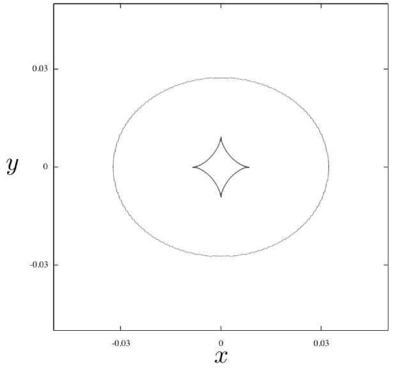
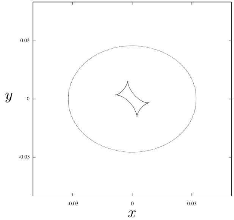
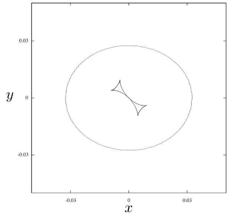
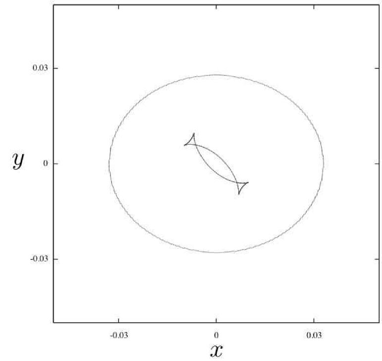
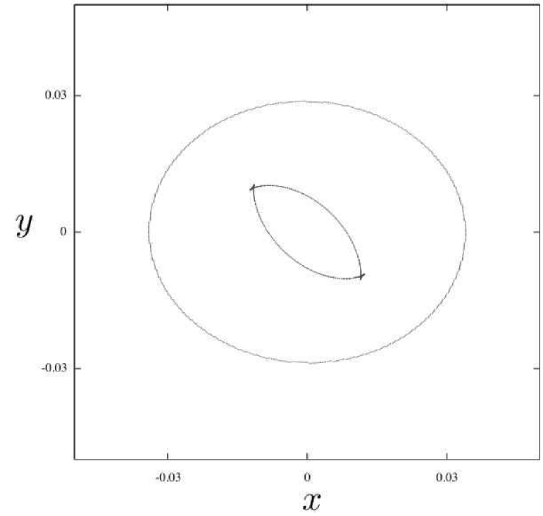
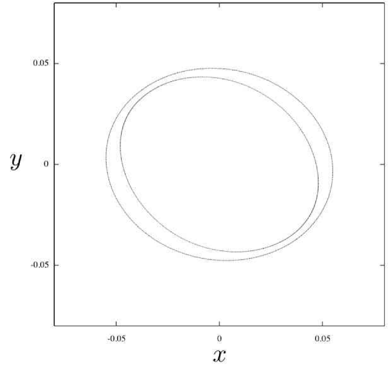
Figure 19: $z=0$ sections of the inner caustics produced by the initial velocity field of Eqs. (18) for $c_{1}=c_{2}=0$, $\xi=0.01$, $g=-0.05$, and increasing values of $c_{3}$: (a) $c_{3}=0$, (b) $c_{3}=0.005$, (c) $c_{3}=0.01$, (d) $c_{3}=0.015$, (e) $c_{3}=0.025$, (f) $c_{3}=0.1$.

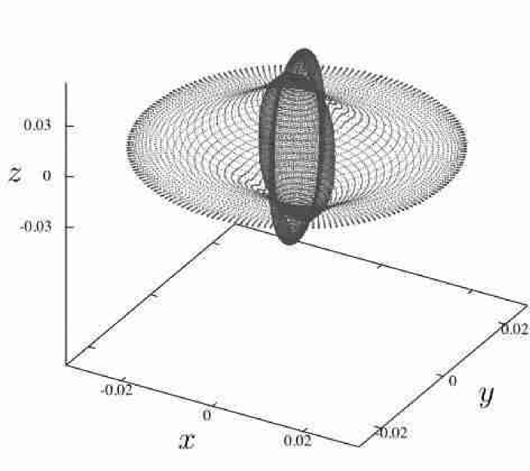
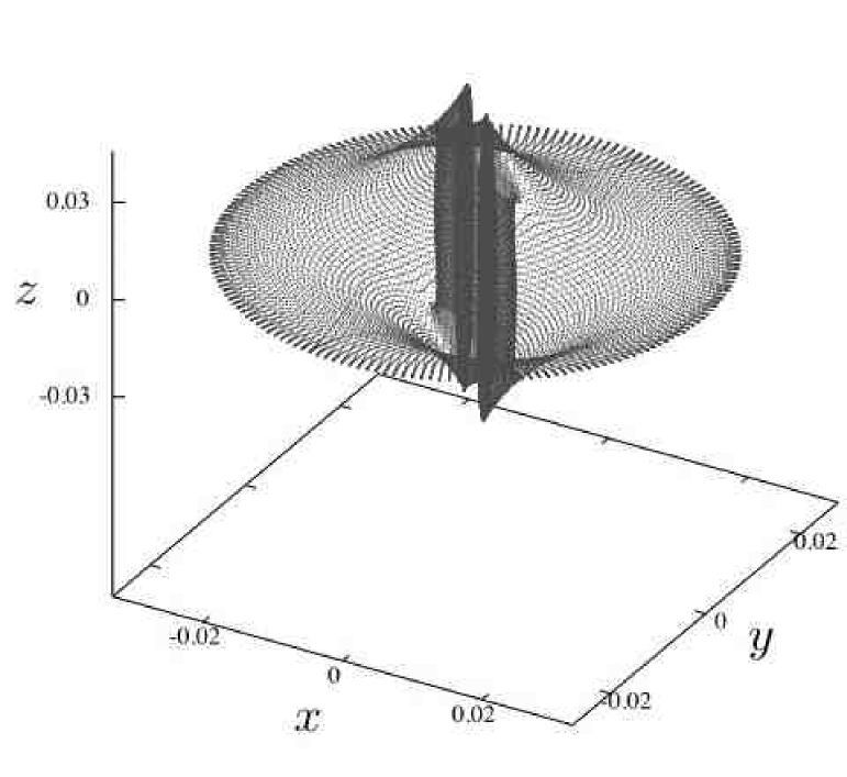
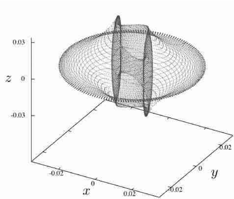
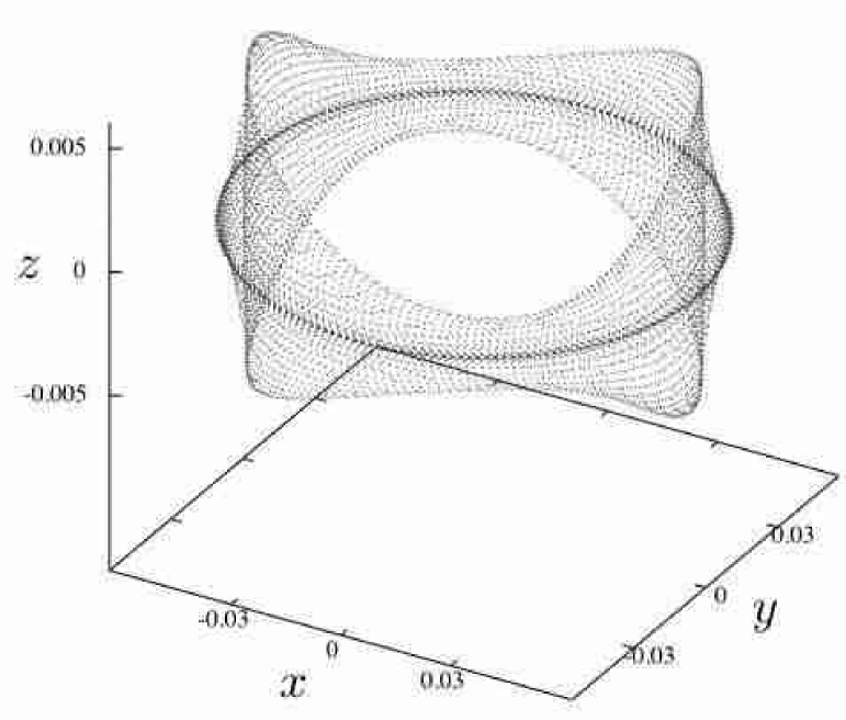
Figure 20: Inner caustics produced by the initial velocity field of Eqs. (18) for $\xi=0.01$, $g=-0.05$, $c_{1}=c_{2}=0$ and increasing values of $c_{3}$: (a) $c_{3}=0$, (b) $c_{3}=0.015$, (c) $c_{3}=0.03$, (d) $c_{3}=0.12$.

Here we add a rotational component ($c_{3}\neq 0$) to the initial velocity field of Eq. (28) to see the metamorphosis of the inner caustic from tent to tricusp ring. Fig. 19 shows the $z=0$ cross sections of the inner caustic during such a transition. In Fig. 19, the initial velocity field is irrotational and we see a circle and diamond, as before. In Fig. 19, the diamond is skewed because of the rotation in the $z=0$ plane introduced by $c_{3}\neq 0$. Fig. 19 shows the case $c_{3}=\xi$. As $c_{3}$ is increased further, the diamond transforms into two swallowtail $(A_{4})$ catastrophes cat joined back to back [19]. There are two flows in the central region, six flows in the cusped region of each swallowtail, four in the other regions inside the circle and two outside the circle. Finally, the swallowtails pinch off to form the inner circle of the $z=0$ section of the tricusp ring. Fig. 20 shows the transition in three dimensions.

VI Conclusions

In Section II, we gave a mathematical proof of the statement that a cold flow of collisionless particles from all directions in and out of a region necessarily produces a caustic. We call this caustic the “inner caustic” of the in and out flow. The main purpose of our paper was to determine the catastrophe structure of the inner caustics formed by cold dark matter particles falling in and out of a galactic gravitational potential well.

The structure of the inner caustic depends for the most part on the angular momentum distribution of the particles falling in. It had been shown previously by analytical methods sing that the inner caustic is a tricusp ring when the velocity distribution of the infalling particles is dominated by net overall rotation. However we show in Section III that the leading theory for the angular momentum of galaxies, namely tidal torque theory, predicts that the velocity field is irrotational $(\vec{\nabla}\times\vec{v}=0)$ to all orders of perturbation theory, i.e. to all orders in an expansion in powers of the size of density perturbations. So, tidal torque theory states not only that the initial velocity field of the infalling particles is not dominated by net overall rotation, it states that the initial velocity field is exactly irrotational.

So the question was: what is the structure of the inner caustic when the initial velocity field is irrotational? Or more generally, what is that structure when the initial velocity field is not dominated by net overall rotation? We addressed this issue by simulating the flow of cold collisionless particles falling in and out of a fixed gravitational potential. In principle we can do this for any initial velocity field. However, we restricted ourselves to initial velocity fields of the form $\vec{v}=M\vec{x}$ where $\vec{x}$ is initial position and $M$ is a $3\times 3$ real traceless matrix. As far as uncovering the catastrophe structure of inner caustics is concerned, we expect this to be a sufficiently broad set of initial velocity fields. Adding higher order terms to the expansion of $\vec{v}$ in powers of $\vec{x}$ is expected to merely deform the inner caustics obtained when keeping linear terms only. $M$ can be written in the form of Eq. (17) which depends on five parameters: $\vec{c}=(c_{1},c_{2},c_{3})$, $g_{1}$ and $g_{2}$. The first three describe net rotation with angular velocity $\vec{c}$. The last two describe irrotational flow.

In Section IV, we simulated flows which are dominated by net rotation and confirm that the inner caustic is a tricusp ring in that case. We show that the tricusp ring is stable under perturbations both in the initial velocity field and in the gravitational potential. This stability is not a surprise since it is known that the structure of non-degenerate catastrophes is stable under perturbations Vakif . When the initial velocity field and/or the gravitational potential are not axially symmetric, the dimensions of the tricusp vary along the ring. In the neighborhood of a point where the tricusp dimensions have shrunk to zero, the catastrophe structure is the full elliptic umbilic.

In Section V, we simulated flows which are not dominated by a rotational component. We started off simulating flows which are both irrotational ($\vec{c}=0$) and axially symmetric ($g_{1}=g_{2}$). For such flows the inner caustic is shown in Fig. 10 for $|g_{1}|<g_{1*}\simeq 0.05$. We call this structure a “tent caustic”. It has a caustic line on the axis of symmetry, which we call the “tent pole”, connected to a caustic surface which we call the “tent roof”. When $g_{1}<-g_{1*}$, the inner caustic is the same as for $|g_{1}|<g_{1*}$ except the cusp in the equatorial plane is replaced by a butterfly caustic. When $g_{1}>g_{1*}$, the cusps on the symmetry axis are replaced by butterfly caustics.

When $g_{2}$ is different from but close to $g_{1}$, axial symmetry is slightly broken. In that case the caustic pole spreads onto a tube whose cross section has four cusps forming a diamond shape. See Figs. 14 and 15. In a region where the tent pole connects with the tent roof, two hyperbolic umbilic catastrophes appear, as described in Fig. 17. Fig. 18 shows what happens when $g_{2}$ is very different from $g_{1}$. The inner caustic metamorphoses from a tent which is symmetric about the $z$ axis when $g_{2}=g_{1}$ to a tent symmetric about the $x$ axis when $g_{2}=-{1\over 2}g_{1}$.

Finally, we investigated the smooth transformation of the tent caustic into a tricusp ring when a rotational component is added ($\vec{c}\neq 0$). In the axially symmetric case (see Fig. 13) the tent pole spreads onto a tube of circular cross section. The radius of this tube becomes the inner radius of the tricusp ring. So, in the axially symmetric case, we may think of the tent caustic as a tricusp ring whose inner radius has shrunk to zero. In the non axially symmetric case, the metamorphosis of tent caustic to tricusp ring is shown in Figs. 19 and  20. The diamond shaped cross section of the tent pole transforms to a (topological) circle by passing through an intermediate stage where it consists of two swallowtail catastrophes back to back.

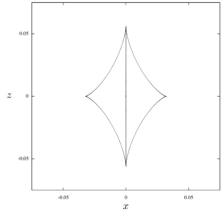
(a) Caustic structure.

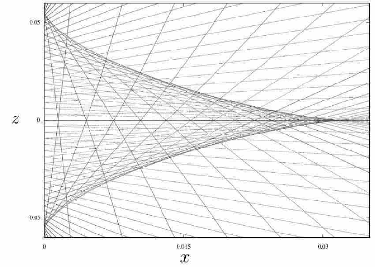
(b) Dark matter flows.

Figure 10: Cross section of the inner caustic produced by the irrotational axially symmetric velocity field $\vec{v}=-0.05\sin\,2\theta\;\hat{\theta}$.

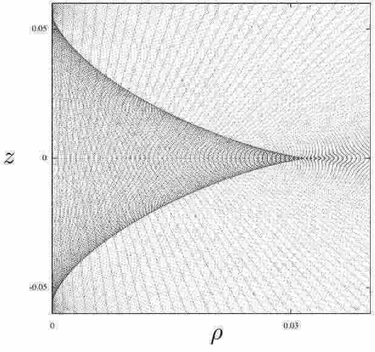
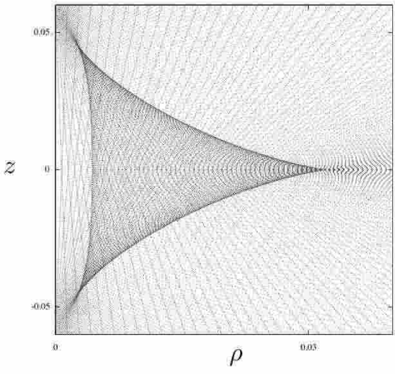
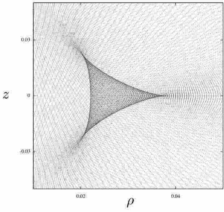
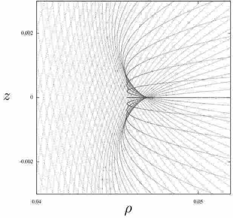
Figure 13: Cross sections of the inner caustics produced by the axially symmetric initial velocity field of Eq. (27) with $g_{1}=-0.033$, and (a) $c_{1}=0$, (b) $c_{2}=0.01$, (c) $c_{3}=0.05$, (d) $c_{3}=0.1$. Increasing the rotational component of the initial velocity field causes the tent caustic (a) to transform into a tricusp ring (d).

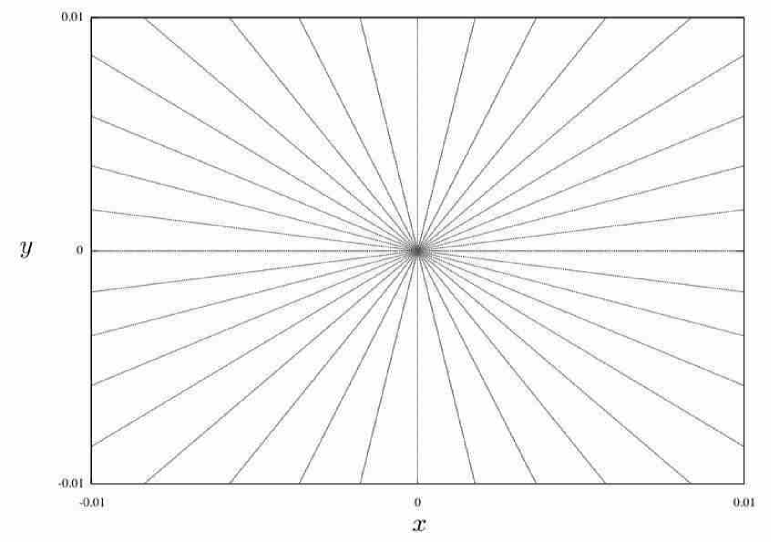
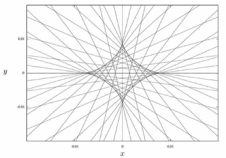
Figure 14: Dark matter flows in the $z=0$ plane for the initial velocity field of Eq. (28) when (a) $\xi=0,g=-0.05$, and (b) $\xi=0.01,g=-0.05$. In (a) the particles move on radial orbits. In (b) the particles have angular momentum about the $z$ axis.

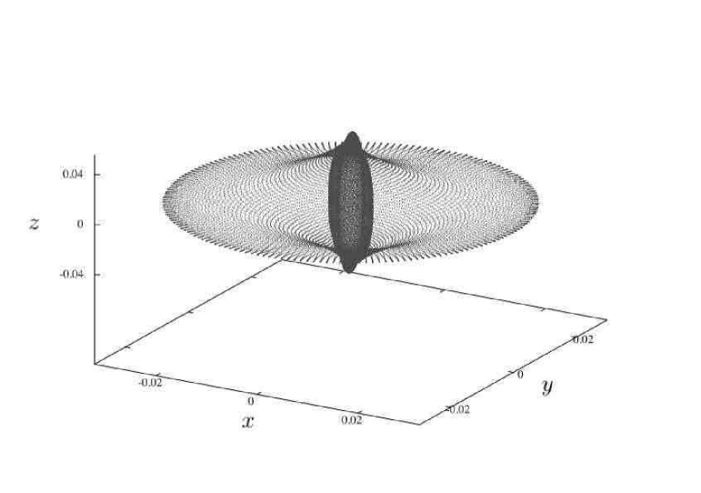
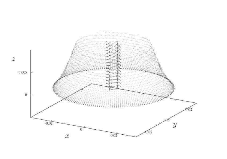
Figure 15: The inner caustic for the initial velocity field of Eq. (28) with $\xi=0.005,g=-0.05$: (a) the tent caustic in 3 dimensions; (b) a succession of constant $z$ sections over the range $0\leq z\leq 0.01$.

- (1) C.L. Bennett et al., Ap. J. Suppl. 148 (2003) 1.
- (2) D. Lynden-Bell, MNRAS 136 (1967) 101.
- (3) P. Salucci, astro-ph/0510123.
- (4) P. Sikivie and J.R. Ipser, Phys. Lett. B291 (1992) 288.
- (5) A. Natarajan and P. Sikivie, Phys. Rev. D72 (2005) 083513.
- (6) J.F. Navarro, C.S. Frenk and S.D.M. White, Ap. J. 462 (1996) 563; B. Moore et al., Ap. J. Lett. 499 (1998) L5.
- (7) A.L. Melott, S.F. Shandarin, R.J. Splinter and Y. Suto, Ap. J. 479 (1997) L79; T. Baertschiger, M. Joyce and F.S. Labini, Ap. J. 581 (2002) L63; J. Diemand, B. Moore, J. Stadel and S. Kazantzides, MNRAS 348 (2004) 977; A.A. El-Zant, astro-ph/0506617.
- (8) P. Sikivie, Phys. Rev. D60 (1999) 063501.
- (9) S. Tremaine, MNRAS 307 (1999) 877.
- (10) J.A. Filmore and P. Goldreich, Ap. J. 281 (1984) 1.
- (11) E. Bertschinger, Ap.J. Suppl. 58 (1985) 39.
- (12) Textbooks on Catastrophe Theory include: P. Saunders, An Introduction to Catastrophe Theory, Cambridge University Press, 1980; R. Gilmore, Catastrophe Theory for Scientists and Engineers, John Wiley and Sons, 1981; V.I. Arnold, Catastrophe Theory, Springer-Verlag, 1992; T. Poston and I. Stewart, Catastrophe Theory and its Applications, Dover reprints, 1996.
- (13) P.J.E. Peebles, Ap.J. 155 (1969) 393.
- (14) A.G. Doroshkevich, Astrofisika 6 (1970) 581.
- (15) S.D. White, Ap.J. 286 (1984) 38.
- (16) For a recent discussion, see e.g. J.R. Primack, IAS Symposium 220 (2004) 467.
- (17) Y.B. Zel’dovich, Astr. Ap. 5 (1970) 84.
- (18) P. Sikivie, I. Tkachev and Y. Wang, Phys. Rev. Lett. 75 (1995) 2911; Phys. Rev. D56 (1997) 1863.
- (19) J. Navarro, C. Frenk and S. White, in ref. Nsim
- (20) P. Saunders, in ref. cat .
- (21) R. Blandford and R. Narayan, Ap. J. 310 (1986) 568.
- (22) A.O. Petters, J. Math. Phys. 34 (1993) 3555.
- (23) A.O. Petters, H. Levine and J. Wambsganss, Singularity Theory and Gravitational Lensing, Birkhauser, 2001.
- (24) T. Poston and I. Stewart, in ref. cat .
- (25) E.C. Zeeman, Catastrophe Theory: Selected Papers (1972-1977), Addison Wesley, 1977;
- (26) For a recent discussion, see V. Onemli, astro-ph/0510414.