Reconstruction of $5D$ Cosmological Models From Equation of State of Dark Energy

Abstract

We consider a class of five-dimensional cosmological solutions which contains two arbitrary function $\mu(t)$ and $\nu(t)$. We found that the arbitrary function $\mu(t)$ contained in the solutions can be rewritten in terms of the redshift $z$ as a new arbitrary function $f(z)$. We further showed that this new arbitrary function $f(z)$ could be solved out for four known parameterized equations of state of dark energy. Then the $5D$ models can be reconstructed and the evolution of the density and deceleration parameters of the universe can be determined.

1 Introduction

Recent observations of high redshift Type Ia supernovae reveal that our universe is undergoing an accelerated expansion rather than decelerated expansion [1, 2, 3]. Meanwhile, the discovery of Cosmic Microwave Background (CMB) anisotropy on degree scales together with the galaxy redshift surveys indicate $\Omega_{total}\simeq 1$ [4] and $\Omega_{m}\simeq\left.1\right/3$. All these results strongly suggest that the universe is permeated smoothly by ’dark energy’, which violates the strong energy condition with negative pressure and causes the expansion rate of the universe accelerating. The dark energy and accelerating universe have been discussed extensively from different points of view [5, 6, 7]. In principle, a natural candidate for dark energy could be a small cosmological constant. However, there exist serious theoretical problems: fine tuning and coincidence problems. To overcome the coincidence problem, some self-interact scaler fields $\phi$ with an equation of state (EOS) $w_{\phi}=p_{\phi}\left/\rho_{\phi}\right.$ were introduced dubbed quintessence, where $w_{\phi}$ is time varying and negative. Generally, the potentials of the scalar field should be determined from the underlying physical theory, such as Supergravity, Superstring/M-theory etc.. However, from the phenomenal level, one can also design many kinds of potentials to solve the concrete problems [5, 8]. Once the potentials are given, EOS $w_{\phi}$ of dark energy can be found. On the other hand, the potential can also be reconstructed from a given EOS $w_{\phi}$ [9]. That is, the forms of the scalar potential can be determined from observational data. Although there are many kinds of models for dark energy, one still knew little about it’s properties. And, one also needs some mechanism to distinguish these different models. Therefore, one may wish to use the model independent method to study the universe without specifying a particular model for dark energy. That is, we can use observational data to parameterize the EOS of dark energy, and then to study the evolution of the universe directly.

The idea that our world may have more than four dimensions is due to Kaluza [10], who unified Einstein’s theory of General Relativity with Maxwell’s theory of Electromagnetism in a $5D$ manifold. In 1926, Klein reconsidered Kaluza’s idea and treated the extra dimension as a compact small circle topologically [11]. Afterwards, the Kaluza-Klein idea has been studied extensively from different points of view. Among them, a kind of theory called Space-Time-Matter (STM) theory, is designed to incorporate the geometry and matter by Wesson and his collaborators (for review, please see [12] and references therein). In STM theory, our $4D$ world is a hypersurface embedded in a $5D$ Ricci flat ($R_{AB}=0$) manifold, and all the matter in our $4D$ world are induced from the extra dimension. This theory is supported by Campbell’s theorem [13] which says that any analytical solution of Einstein field equation of $N$ dimensions can be locally embedded in a Ricci-flat manifold of $\left(N+1\right)$ dimensions. Since the matter are induced from the extra dimension, this theory is also called induced matter theory.

Within the framework of STM theory, a cosmological solution is presented in [14] in which it was shown that the universe is characterized by having a big bounce instead of a big bang. It was also shown that both the radiation and matter dominated cosmological models could be recovered from the solution. Further studies of this solution include the embedding to brane models [15], the isometry with $5D$ black holes [16], the big bounce singularity [17], and the dark energy models [18, 20]. The purpose of this paper is to study the acceleration of the $5D$ solution. The solution contains two arbitrary functions $\mu(t)$ and $\nu(t)$. We will show in Section 2 that one of these two arbitrary functions, $\mu(t)$, plays a similar role as the potential $V\left(\phi\right)$ in quintessence or phantom dark energy models. This enable us to study the evolution of the $5D$ universe in a model independent way. We will reconstruct the evolution of the $5D$ universe by using four known parameterized methods. Section 3 is a short discussion.

2 Dark energy in a class of five-dimensional cosmological model

The $5D$ cosmological solution was originally given by Liu and Mashhoon in 1995 [19]. Then, in 2001, Liu and Wesson [14] restudied the solution and showed that it describes a cosmological model with a big bounce as opposed to a big bang. The $5D$ metric of this solution reads

$$dS^{2}=B^{2}dt^{2}-A^{2}\left(\frac{dr^{2}}{1-kr^{2}}+r^{2}d\Omega^{2}\right)-dy^{2}$$ (1)

where $d\Omega^{2}\equiv\left(d\theta^{2}+\sin^{2}\theta d\phi^{2}\right)$ and

$$A^{2} = \left(\mu^{2}+k\right)y^{2}+2\nu y+\frac{\nu^{2}+K}{\mu^{2}+k},$$

$$B = \frac{1}{\mu}\frac{\partial A}{\partial t}\equiv\frac{\dot{A}}{\mu}.$$ (2)

Here $\mu=\mu(t)$ and $\nu=\nu(t)$ are two arbitrary functions of $t$, $k$ is the $3D$ curvature index $\left(k=\pm 1,0\right)$, and $K$ is a constant. This solution satisfies the 5D vacuum equation $R_{AB}=0$. So, the three invariants are

$$I_{1} \equiv R=0,I_{2}\equiv R^{AB}R_{AB}=0,$$

$$I_{3} = R_{ABCD}R^{ABCD}=\frac{72K^{2}}{A^{8}}.$$ (3)

The invariant $I_{3}$ in Eq. (3) shows that $K$ determines the curvature of the 5D manifold.

Using the $4D$ part of the $5D$ metric (1) to calculate the $4D$ Einstein tensor, one obtains

$${}^{(4)}G_{0}^{0} = \frac{3\left(\mu^{2}+k\right)}{A^{2}},$$

$${}^{(4)}G_{1}^{1} = {}^{(4)}G_{2}^{2}=^{(4)}G_{3}^{3}=\frac{2\mu\dot{\mu}}{A\dot{A}}+\frac{\mu^{2}+k}{A^{2}}.$$ (4)

In Ref. [20], the induced matter was set to contain three components: dark matter, radiation and $x$-matter. In this paper, we assume, for simplicity, the induced matter to contain two parts: cold dark matter (CDM) $\rho_{cd}$ and dark energy (DE) $\rho_{de}$. So, we have

$$\frac{3\left(\mu^{2}+k\right)}{A^{2}} = \rho_{cd}+\rho_{de},$$

$$\frac{2\mu\dot{\mu}}{A\dot{A}}+\frac{\mu^{2}+k}{A^{2}} = -\left(p_{cd}+p_{de}\right),$$ (5)

where

$$p_{cd}=0,\quad p_{de}=w_{de}\rho_{de}.$$ (6)

From Eqs.(5) and (6), one obtains the EOS of the dark energy

$$w_{de}=\frac{p_{de}}{\rho_{de}}=-\frac{2\left.\mu\dot{\mu}\right/A\dot{A}+\left.\left(\mu^{2}+k\right)\right/A^{2}}{3\left.\left(\mu^{2}+k\right)\right/A^{2}-\rho_{cd0}A^{-3}},$$ (7)

and the dimensionless density parameters

$$\Omega_{cd} = \frac{\rho_{cd}}{\rho_{cd}+\rho_{de}}=\frac{\rho_{cd0}}{3\left(\mu^{2}+k\right)A},$$ (8)

$$\Omega_{de} = 1-\Omega_{cd}.$$ (9)

where $\rho_{cd0}=\bar{\rho}_{cd0}A_{0}^{3}$ ($\bar{\rho}_{cd0}$ and $A_{0}$ denote the current density of CDM and scale factor at present time, respectively (The subscript $0$ denotes value at present time), and $\Omega_{cd}$ and $\Omega_{de}$ are dimensionless density parameters of CDM and DE, respectively. The Hubble parameter and deceleration parameter should be given as [14], [20],

$$H \equiv \frac{\dot{A}}{AB}=\frac{\mu}{A}$$ (10)

$$q\left(t,y\right) \equiv \left.-A\frac{d^{2}A}{d\tau^{2}}\right/\left(\frac{dA}{d\tau}\right)^{2}=-\frac{A\dot{\mu}}{\mu\dot{A}},$$ (11)

from which we see that $\dot{\mu}\left/\mu\right.>0$ represents an accelerating universe, $\dot{\mu}\left/\mu\right.<0$ represents a decelerating universe. So the function $\mu(t)$ plays a crucial role in defining the properties of the universe at late time. In this paper, we consider the spatially flat $k=0$ cosmological model. From equations (7)-(11), it is easy to see that these equations do not contain the second arbitrary $\nu(t)$ explicitly. So if we use the relation

$$A_{0}\left/A\right.=1+z$$ (12)

and define $\mu_{0}^{2}\left/\mu_{z}^{2}\right.=f\left(z\right)$ with $f(0)\equiv 1$, then these equations (7)-(11) can be expressed in terms of redshift $z$ as

$$w_{de} = -\frac{1+\left(1+z\right)d\ln f\left(z\right)\left/dz\right.}{3-3\Omega_{cd}},$$ (13)

$$\Omega_{cd} = \Omega_{cd0}\left(1+z\right)f\left(z\right),$$ (14)

$$\Omega_{de} = 1-\Omega_{cd},$$ (15)

$$H^{2} = H_{0}^{2}(1+z)^{2}f(z)^{-1},$$ (16)

$$q = \frac{1+3\Omega_{de}w_{de}}{2}=-\frac{\left(1+z\right)}{2}\frac{d\ln f\left(z\right)}{dz}.$$ (17)

Note that in the $5D$ bounce model the scale factor $A$ reaches a nonzero minimum at $t=t_{b}$ where $t_{b}$ is the bouncing time. From Eq. (12), this $t_{b}$ corresponds to a maximum redshift $z_{b}$. Therefore, the relation (12) and all the equations after it only valid in the range $z<z_{b}$ (i.e., after the bounce).

Now let us consider equation (13) which is a first order ordinary differential equation of the function $f(z)$ w.r.t. redshift $z$. This equation could be integrated if the form of $w_{de}(z)$ is given. It was shown in [9] that the scalar potentials can be constructed from a given EOS of dark energy $w_{\phi}$. Following this spirit, we can also reconstruct the forms of function $f(z)$ from a given concrete form of $w_{de}(z)$. And once the function $f(z)$ is constructed, the evolution of the universe can be determined. At this point, we say that the cosmological models are reconstructed.

Following Ref.[9], we consider the following four cases to reconstruct the forms of $f(z)$.

Case I: $w_{de}=w_{0}$ (Ref. [21]) For this case, $w_{de}$ is a constant and we find that Eq. (13) can be integrated, giving

$$f(z)=\frac{1}{(1+z)\left(\Omega_{cd0}+\Omega_{de0}(1+z)^{3w_{0}}\right)}.$$ (18)

Then using this $f(z)$ in (14), (15) and (17), we obtain $\Omega_{cd}$, $\Omega_{de}$ and $\Omega_{q}$ expressed in terms of $z$ alone. The evolutions of the dimensionless energy density parameters $\Omega_{cd}$ and $\Omega_{de}$, EOS of dark energy $\omega_{de}$, and the deceleration parameter $q$ are plotted in Fig. (1).

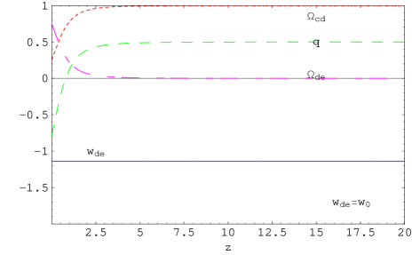
Figure 1: Case I: The evolution of the dimensionless density parameters $\Omega_{cd}$, $\Omega_{de}$, and deceleration parameter $q$, EOS of dark energy $w_{de}$ versus redshift $z$, where $\Omega_{cd0}=0.25$, $\Omega_{de0}=0.75$, and $\omega_{0}=-1.14$.

Case II: $w_{de}=w_{0}+w_{1}z$ (Ref. [22]) For this case Eq. (13) can also be integrated, giving

$$f(z)=\frac{(1+z)^{3w_{1}-1}}{\Omega_{cd0}(1+z)^{3w_{1}}+\Omega_{de0}(1+z)^{3w_{0}}\exp(3w_{1}z)}.$$ (19)

Using this $f(z)$ in (14), (15) and (17), we obtain the expressions of the evolutions of the dimensionless energy density parameters $\Omega_{cd}$ and $\Omega_{de}$, EOS of dark energy $\omega_{de}$, and the deceleration parameter $q$, and we plot them in Fig. (2).

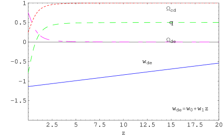
Figure 2: Case II: The evolution of the dimensionless density parameters $\Omega_{cd}$, $\Omega_{de}$, and deceleration parameter $q$, EOS of dark energy $w_{de}$ versus redshift $z$, where $\Omega_{cd0}=0.25$, $\Omega_{de0}=0.75$, $\omega_{0}=-1.14$ and $\omega_{1}=0.03$.

Case III: $w_{de}=w_{0}+w_{1}\frac{z}{1+z}$ (Ref. [23, 24]) Similar as in case I and case II, for this case we have

$$f(z)=\frac{1}{(1+z)\left[\Omega_{cd0}+\Omega_{de0}(1+z)^{3w_{0}+3w_{1}}\exp(-\frac{3w_{1}z}{1+z})\right]}.$$ (20)

We plot the evolutions of the dimensionless energy density parameters $\Omega_{cd}$ and $\Omega_{de}$, EOS of dark energy $\omega_{de}$ and deceleration parameter $q$ in Fig. (3).

Figure 3: Case III: The evolution of the dimensionless density parameters $\Omega_{cd}$, $\Omega_{de}$, and deceleration parameter $q$, EOS of dark energy $w_{de}$ versus redshift $z$, where $\Omega_{cd0}=0.25$, $\Omega_{de0}=0.75$, $\omega_{0}=-1.14$ and $\omega_{1}=1.1$.

Case IV: $w_{de}=w_{0}+w_{1}\ln(1+z)$ (Ref. [25]) For this case $f(z)$ is also integrable and we find

$$f(z)=\frac{1}{(1+z)\left[\Omega_{cd0}+\Omega_{de0}(1+z)^{3w_{0}}\exp(\frac{3w_{1}\ln(1+z)^{2}}{2})\right]}.$$ (21)

We plot the evolutions of the dimensionless energy density parameters $\Omega_{cd}$ and $\Omega_{de}$, EOS of dark energy $\omega_{de}$ and deceleration parameter $q$ in Fig. (4).

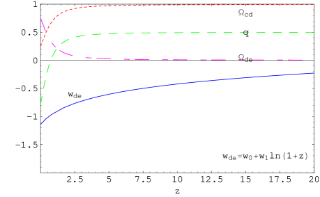
Figure 4: Case IV: The evolution of the dimensionless density parameters $\Omega_{cd}$, $\Omega_{de}$, and deceleration parameter $q$, EOS of dark energy $w_{de}$ versus redshift $z$, where $\Omega_{cd0}=0.25$, $\Omega_{de0}=0.75$, $\omega_{0}=-1.14$ and $\omega_{1}=0.3$.

We see that in Case I the EOS of dark energy $w_{de}$ is assumed to be a constant $w_{0}$ during the whole evolution of the universe. In the other three cases, $w_{de}$ deviates from $w_{0}$ in different ways as the redshift $z$ increases. This causes the density and deceleration parameters $\Omega_{cd}$, $\Omega_{de}$ and $q$ deviate from those in Case I explicitly at higher redshift. It is expected that these deviations may become very large at very large redshift. In further studies we are going to use more observational dada such as those from the SNe Ia data to constrain the parameters in the expression of $w_{de}$. Here, in this paper, we just want to use above four cases to illustrate how to reconstruct function $f(z)$ from a given EOS of dark energy, and the results show that our procedure works.

3 Discussion

The $5D$ cosmological solution presented by Liu, Mashhoon and Wesson in [19] and[14] is rich in mathematics because it contains two arbitrary functions $\mu(t)$ and $\nu(t)$. However, this also brings us a problem: how to determine the two arbitrary functions. In this paper we find that one of the two functions, $\mu(t)$, plays a similar role as the potential $V(\phi)$ in the quintessence and phantom dark energy models. Meanwhile, another arbitrary function $\nu(t)$ seems do not affect the densities and the EOS of dark energy in an explicit way. This reminds us of a similar situation happened in the $4D$ general relativity where one can study the cosmic evolution of dark energy (as well as other densities) just from a given parameterized EOS of dark energy without knowing it’s explicit form and without knowing the explicit form of the scale factor $a(t)$. Following this kind of model independent methods we have used the relation (12) and successfully derived the differential equation (13) which governs the function $f(z)$. Furthermore, for four known EOS of dark energy, we have successfully integrated Eq. (13) and plotted the evolutions of the density and deceleration parameters $\Omega_{cd}$, $\Omega_{de}$ and $q$. In this sense, we say that we have reconstructed the $5D$ solution. However, we should also say that this kind of reconstruction is not complete. As we mentioned in Section 2 that the relation $A(z)=A_{0}(1+z)^{-1}$ in (12) does not cover the whole $5D$ manifold of the bounce solution; it can only cover ”half” of it, i.e., that half after the bounce for $z<z_{b}$. There is actually a one to two correspondence between $A$ and $t$ for the whole curve of $A$ in the bounce model; while the relation $A(z)=A_{0}(1+z)^{-1}$ is just a one to one correspondence between $A$ and $z$. On the other hand, even if in the $4D$ general relativity, the scale factor $a(t)$ is not easy to be integrated out analytically if the cosmic matter contains more than one different components of matter. In our $5D$ case, the scale factor $A(t,y)$ might be more complicated than $a(t)$. To study the evolution of the whole bounce model, one may need look for other method such as the numerical simulation which beyond the scope of this paper.

4 Acknowledgments

This work was supported by NSF (10273004) and NBRP (2003CB716300) of P. R. China.

References

- [1] A.G. Riess, et.al., Observational evidence from supernovae for an accelerating universe and a cosmological constant, Astron. J. 116 1009 (1998), astro-ph/9805201; S. Perlmutter, et.al., Measurements of omega and lambda from 42 high-redshift supernovae, Astrophys. J. 517 565 (1999), astro-ph/9812133.
- [2] J.L. Tonry, et.al., Cosmological Results from High-z Supernovae , Astrophys. J. 594 1 (2003), astro-ph/0305008; R.A. Knop, et.al., New Constraints on , , and w from an Independent Set of Eleven High-Redshift Supernovae Observed with HST, astro-ph/0309368; B.J. Barris, et.al., 23 High Redshift Supernovae from the IfA Deep Survey: Doubling the SN Sample at z¿0.7, Astrophys.J. 602 571 (2004), astro-ph/0310843.
- [3] A.G. Riess, et.al., Type Ia Supernova Discoveries at From the Hubble Space Telescope: Evidence for Past Deceleration and Constraints on Dark Energy Evolution, astro-ph/0402512.
- [4] P. de Bernardis, et.al., A Flat Universe from High-Resolution Maps of the Cosmic Microwave Background Radiation, Nature 404 955 (2000), astro-ph/0004404; S. Hanany, et.al., MAXIMA-1: A Measurement of the Cosmic Microwave Background Anisotropy on angular scales of 10 arcminutes to 5 degrees, Astrophys. J. 545 L5 (2000), astro-ph/0005123; D.N. Spergel et.al., First Year Wilkinson Microwave Anisotropy Probe (WMAP) Observations: Determination of Cosmological Parameters, Astrophys. J. Supp. 148 175(2003), astro-ph/0302209.
- [5] I. Zlatev, L. Wang, and P.J. Steinhardt , Quintessence, Cosmic Coincidence, and the Cosmological Constant, Phys. Rev. Lett. 82 896 (1999), astro-ph/9807002; P.J. Steinhardt, L. Wang , I. Zlatev, Cosmological Tracking Solutions, Phys. Rev. D59 123504 (1999), astro-ph/9812313; M.S. Turner , Making Sense Of The New Cosmology, Int. J. Mod. Phys. A17S1 180 (2002), astro-ph/0202008; V. Sahni , The Cosmological Constant Problem and Quintessence, Class.Quant.Grav. 19 3435 (2002), astro-ph/0202076.
- [6] R.R. Caldwell, M. Kamionkowski, N.N. Weinberg, Phantom Energy: Dark Energy with w Causes a Cosmic Doomsday, Phys. Rev. Lett. 91 071301 (2003), astro-ph/0302506; R.R. Caldwell , A Phantom Menace? Cosmological consequences of a dark energy component with super-negative equation of state, Phys. Lett. B545 23 (2002), astro-ph/9908168; P. Singh, M. Sami, N. Dadhich, Cosmological dynamics of a phantom field, Phys. Rev. D68 023522 (2003), hep-th/0305110; J.G. Hao, X.Z. Li , Attractor Solution of Phantom Field, Phys.Rev. D67 107303 (2003), gr-qc/0302100.
- [7] Armendáriz-Picón, T. Damour, V. Mukhanov, k-Inflation, Physics Letters B458 209 (1999); M. Malquarti, E.J. Copeland , A.R. Liddle, M. Trodden, A new view of k-essence, Phys. Rev. D67 123503 (2003); T. Chiba , Tracking k-essence, Phys. Rev. D66 063514 (2002), astro-ph/0206298.
- [8] V. Sahni, Theoretical models of dark energy, Chaos. Soli. Frac. 16 527 (2003).
- [9] Z.K. Guo, N. Ohtab and Y.Z. Zhang, Parametrization of Quintessence and Its Potential, astro-ph/0505253.
- [10] T. Kaluza, On The Problem Of Unity In Physics, Sitzungsber. Preuss. Akad. Wiss. Berlin (Math. Phys.) K1 966 (1921).
- [11] O. Klein, Quantum Theory And Five-Dimensional Relativity, Z. Phys. 37 895 (1926) [Surveys High Energ. Phys. 5 241 (1926)].
- [12] P.S. Wesson, Space-Time-Matter (Singapore: World Scientific) 1999; J. Ponce de Leon, Mod. Phys. Lett. A16 2291 (2001), gr-qc/0111011.
- [13] J.E. Campbell, A Course of Differential Geometry, (Clarendon Oxford, 1926); S. Rippl, R. Romero, R. Tavakol, Gen. Quantum Grav. 12 2411 (1995); C. Romero, R. Tavako and R. Zalaletdinov, Ge. Relativ. Gravit. 28 365 (1996); J. E.Lidsey, C. Romero, R. Tavakol and S. Rippl, Class. Quantum Grav. 14 865 (1997); S.S. Seahra and P.S. Wesson, Application of the Campbell-Magaard theorem to higher-dimensional physics, Class. Quant. Grav. 20 1321 (2003), gr-qc/0302015.
- [14] H. Y. Liu and P. S. Wesson, Universe models with a variable cosmological “constant” and a “big bounce”, 2001 Astrophys. J. 562 1, gr-qc/0107093;
- [15] S.S. Seahra, Phys. Rev. D68, 104027 (2003), hep-th/0309081; S.S. Seahra, P. S. Wesson, Class. Quant. Grav. 20, 1321 (2003), gr-qc/0302015; J. Ponce de Leon, Mod. Phys. Lett. A16, 2291 (2001), gr-qc/0111011; H.Y. Liu, Phys. Lett. B560, 149 (2003), hep-th/0206198.
- [16] S. S. Seahra and P. S. Wesson, J.Math.Phys. 44 5664 (2003), gr-qc/0309006; The universe as a five-dimensional black hole, preprint, University of Waterloo (2005).
- [17] L.X. Xu , H.Y. Liu, B.L. Wang, Big Bounce singularity of a simple five-dimensional cosmological model, Chin. Phys. Lett. 20 995 (2003), gr-qc/0304049;
- [18] B.L. Wang, H.Y. Liu, L.X. Xu, Accelerating Universe in a Big Bounce Model, Mod. Phys. Lett. A19 449 (2004), gr-qc/0304093; L.X. Xu, H.Y. Liu, Scaling Dark Energy in a Five-Dimensional Bouncing Cosmological Model to appear in Int. J. Mod. Phys. D, astro-ph/0507250; H.Y. Liu, H.Y. Liu, B.R. Chang, L.X. Xu, Induced Phantom and 5D Attractor Solution in Space-Time-Matter Theory, Mod. Phys. Lett. A20 1973 (2005), gr-qc/0504021; B.R. Chang, H.Y. Liu, H.Y. Liu, L.X. Xu, Five-Dimensional Cosmological Scaling Solution, Mod. Phys. Lett. A20 923 (2005), astro-ph/0405084; L.X. Xu, H.Y. Liu, The Correspondence Between a Five-dimensional Bounce cosmological Model and Quintessence Dark Energy Models, Mod. Phys. Lett. A21 1 (2006), astro-ph/0507397.
- [19] H.Y. Liu and B. Mashhoon, A machian interpretation of the cosmological constant, Ann. Phys. 4 565 (4995).
- [20] L.X. Xu, H.Y. Liu, Three Components Evolution in a Simple Big Bounce Cosmological Model, Int. J. Mod. Phys. D14 883 (2005), astro-ph/0412241.
- [21] S. Hannestad, E. Mortsell, Phys. Rev. D66 063508 (2002).
- [22] A.R. Cooray and D. Huterer, Astrophys. J. 513 L95 (1999) .
- [23] E.V. Linder, Phys. Rev. Lett. 90 091301 (2003).
- [24] T. Padmanabhan and T.R. Choudhury, Mon. Not. Roy. Astron. Soc. 344 823 (2003).
- [25] B.F. Gerke and G. Efstathiou, Mon. Not. Roy. Astron. Soc. 335 33 (2002).