A Deep XMM–Newton Serendipitous Survey of a middle–latitude area

The radio quiet neutron star 1E1207.4-5209 has been the target of a 260 ks XMM–Newton observation, which yielded, as a by product, an harvest of about 200 serendipitous X–ray sources above a limiting flux of $2\times 10^{-15}$ erg cm^-2 sec^-1, in the 0.3-8 keV energy range. In view of the intermediate latitude of our field ($b\simeq 10^{\circ}$), it comes as no surprise that the log$N$–log$S$ distribution of our serendipitous sources is different from those measured either in the Galactic Plane or at high galactic latitudes. Here we shall concentrate on the analysis of the brightest sources in our sample, which unveiled a previously unknown Seyfert–2 galaxy.

1 Introduction

The radio quiet neutron star 1E1207.4-5209 has been the target of a 260 ks XMM–Newton observation (De Luca et al. 2004). Such an observation ranges amongst the longest ever performed by XMM–Newton and, as of today, is certainly the longest one at intermediate galactic latitude (i.e. $|b|\simeq 10^{\circ}$).

The deepest X–ray surveys performed, such as the Chandra Deep Field South (Giacconi et al. 2001; Rosati et al. 2002; Giacconi et al. 2002) and North (Brandt et al. 2001), as well as the XMM Lockman Hole survey (Hasinger et al. 2001; Mainieri et al. 2002), encompass only high latitude regions, where serendipitous surveys were also performed (Barcons et al. 2002; Della Ceca et al. 2004). On the other hand, X–ray studies of the galactic population have been performed only along the Galactic Plane: shallow, wide–field surveys were obtained by ROSAT (Motch et al. 1998; Morley et al. 2001) and XMM–Newton (Hands et al. 2004), while deep, pencil–beam observations of the Galactic Center have been performed by CHANDRA (Muno et al. 2003).

Thus, our long observation at intermediate latitude appears to be well suited to address important issues such as the ratio between galactic and extragalactic contributors. The combination of the low flux limit, the wide energy band and the relatively low galactic latitude of this field has the potential for an extremely interesting mix of source types. Owing to the high–energy sensitivity of EPIC, we expect to see through the galactic disk to the distant population of QSOs, AGNs and normal galaxies. On top of such an extragalactic population, however, our field also samples in great depth our Galaxy. Here again the wide energy range allows to sample both hard and soft sources, e.g. population of X–ray binaries and normal stars.

Characterization of the sources’ X-ray spectra, as well as the search for their optical counterparts, are the classical tools to identify, either individually or on a statistical ground, our sample of relatively faint sources. Given the range of $f_{x}/f_{opt}$ values characteristic for the known classes of X–ray sources (Krautter et al. 1999), we ought to reach $V\simeq 25$ in the optical follow–up in order to be able to identify the majority of our serendipitous sources. Thus, although useful for a first filtering, Digital Sky Surveys are not deep enough for our purpose and they do not provide an adequate color coverage.

A proposal for the complete optical coverage of the EPIC field at the 2.2 m ESO telescope has already been accepted. Waiting for its results, here we outline our detection technique as well as the global results of such an analysis. Next we shall focus on the analysis of the brightest sources leading to the spectral characterization of a serendipitously discovered Seyfert–2 galaxy.

2 X–ray analysis

2.1 Observations and data processing

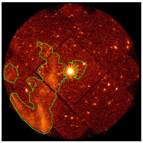
Figure 1: Top: EPIC MOS image (in the energy range 0.3–8 keV) of the field of 1E1207.4-5209. Bottom: Histogram of the count number per pixel in the background map, in the energy range 0.5–2 keV. The sky region corresponding to the tail of the distribution, at values higher than 4, is enclosed by a green line: it is clearly associated to the area of diffuse emission.

XMM–Newton observed 1E1207.4-5209 during revolutions 486 and 487, which resulted in two different pointings separated by $\sim$ 13 h. All the three EPIC focal plane cameras (Turner et al. 2001; Strüder et al. 2001) were active during both pointings: the two MOS cameras were operated in Full Frame mode, in order to cover the whole field–of–view of 30 arcmin; the pn camera was operated in Small Window mode, where only the on–target CCD is read–out, in order to time tag the photons and provide accurate arrival time information. While the pn data have been used by Bignami et al. (2003) and De Luca et al. (2004) to study the radio–quiet neutron–star 1E1207.4-5209, here we shall use the MOS data to assess the population of serendipitous sources emerging from this long galactic observation. For both cameras the thin filter was used.

The event files were processed with the version 5.4.1 of the XMM–Newton Science Analysis Software (SAS). After the standard processing pipeline, we looked for periods of high instrument background, due to flares of protons with energies less than a few hundred keV hitting the detector surface. Such soft proton flares enhance the background and the corresponding time intervals have to be rejected, reducing, accordingly, the good integration time. In our case, the effective observing time was $\sim$ 230 ks over a total observing time of 260 ks.

2.2 Source detection

In order to maximize the signal–to–noise ratio (S/N) of our serendipitous sources and to reach lower flux limits, we ‘merged’ the data of the two cameras and of the two pointings. We performed the source detection in several energy ranges; first, we considered the two ‘classical’, coarse energy ranges 0.5–2 and 2–10 keV; then, we considered a finer energy division between 0.3 and 8 keV (since above 8 keV the instrument effective area decreases rapidly). For each energy band we generated the field image, the corresponding exposure map (to account for the mirror vignetting) and the relevant background map. The background maps were also corrected pixel by pixel, as described in Baldi et al. (2002), in order to reproduce the local variations.

We had also to take into account that the XMM–Newton image includes a region of diffuse emission characterized by more than 4 events/pixel (Fig. 1), due to the SNR G296.5+10.0. Therefore, we performed the source detection with an ‘ad hoc’ tuning of the parameters inside and outside the SNR area.

The source detection was based on the standard maximum detection likelihood criterium: for each source and each energy range we calculated a detection likelihood L=-lnP, where P is the probability that the source counts originate from a background fluctuation. We considered a threshold value $L_{th}$=8.5, corresponding to a probability $P_{th}=2\cdot 10^{-4}$. The actual sky coverage in the various energy ranges was calculated as described in Baldi et al. (2002): in Fig. 2 we show such a coverage for the two coarse energy ranges.

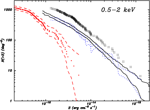
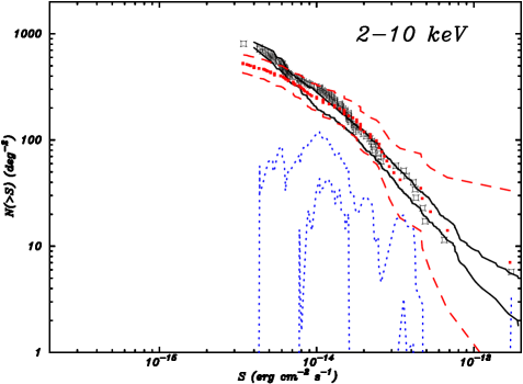
Figure 2: Sky coverage of the performed observation (top), in the energy ranges 0.5–2 keV (solid line) and 2–10 keV (dashed line), and log$N$–log$S$ distribution of the detected sources (black open squares) in the energy ranges 0.5–2 keV (middle) and 2–10 keV (bottom). The black solid lines trace the upper and lower limits obtained by Baldi et al. (2002) in the same energy ranges but at higher galactic latitudes; the blue dotted lines are the difference between our data and the Baldi et al. ones. The red filled squares and the red dashed lines represent, respectively, the distributions and the limits measured by CHANDRA in the galactic plane (Ebisawa et al. 2005).

The number of spurious detections in each energy range, obtained multiplying $P$ times the number of independent (not overlapping) detection cells, is negligible. Indeed, in our detection procedure the area covered by each cell ranges between 0.16 and 0.35 square arcminutes (following the position dependent Point Spread Function size) so that the $\sim$700 square arcmin EPIC field–of–view contains, at most, 5$\times 10^{3}$ detection cells. Thus the number of spurious detection is $P_{th}\times N\leq 1$. Since we performed the source detection in 6 independent energy bands, we expect the total number of spurious detected sources to be at most 6. Selecting all the sources with $L>8.5$ in at least one of our energy ranges and matching those detected in several energy intervals we found a total of 196 sources (with a position accuracy of $\sim$ 5”), 35 inside the area covered by the diffuse emission and 161 outside it. We detected 135 sources between 0.5 and 2 keV and 89 sources between 2 and 10 keV, at a flux limit of $1.3\times 10^{-15}$ and $3.4\times 10^{-15}$ erg cm^-2 s^-1, respectively; 68 of them were detected in both energy bands. In order to evaluate the flux of our sources, we assumed a template AGN spectrum, i.e. a power–law with photon–index $\Gamma$=1.75 and an hydrogen column density N_H of $1.28\times 10^{21}$ cm^-2, corresponding to the total galactic column density.

2.3 Log$N$–Log$S$ distribution

In Fig.2 we show the cumulative log$N$–log$S$ distributions for the sources detected in the two energy ranges. For comparison, we have superimposed to our data the lower and upper limits of the log$N$–log$S$ measured by Baldi et al. (2002) for a survey at high galactic latitude ($|b|>27^{\circ}$): they obtained the upper limit log$N$–log$S$ by applying the same detection threshold ($P_{\rm th}=2\times 10^{-4}$) but a larger extraction radius, while the lower limit log$N$–log$S$ was obtained with the same extraction radius but a more constraining threshold value ($P_{\rm th}=2\cdot 10^{-5}$). Moreover, in the same figure we have also reported the log$N$–log$S$ distributions, as well as the 90 % confidence limits, measured by CHANDRA in the galactic plane (Ebisawa et al. 2005).

In the soft energy band, the log$N$–log$S$ distribution of our sources is well above the high–latitude upper limit, expecially at low X–ray fluxes. Even if the galactic column density represents an overestimate for the stellar population of our sample, we have checked that not all of such an excess can be ascribable to overcorrection for interstellar absorption arising from the use of the total galactic N_H value. We note also that $\sim$ 60 % of the soft sources were not detected in the hard energy band. In the soft band, the galactic plane log$N$–log$S$ distribution (the red points) is much lower than the one at high latitudes, since a significant fraction of extra–galactic sources is not detected. Moreover, the same log$N$–log$S$ is also lower than the difference between our data and the distribution limits at high latitudes (the blue lines). Since Ebisawa et al. (2005) find that most of their soft sources are nearby X–ray active stars, it is possible that our excess over their distribution is due to additional, more distant galactic sources, which are missed looking at $b\sim 0^{\circ}$ but can be detected just outside the galactic plane.

In the hard energy band the distribution of our sources is in good agreement with both the high latitude and the galactic plane ones measured by XMM–Newton, CHANDRA and ASCA (Hands et al. 2004; Ebisawa et al. 2005). At energies $>$ 2 keV we expect the galactic absorption to be negligible so that the extragalactic sources dominate the log$N$–log$S$ distribution at all galactic latitudes, with just a small contribution of the softer galactic sources.

3 Search for optical counterparts

In order to identify our serendipitous X–ray sources, we cross–correlated their positions with two optical catalogues, namely

• the version 2.3 of the Guide Star Catalogue (GSC), not yet published, with limiting magnitudes $B_{J}\sim 23$ and $F\sim 22$, photometric accuracy of $\sim$ 0.25 mag for $B_{J}$ and $\sim$ 0.2 mag for $F$, and position errors $<$ 0.5” (Chieregato et al. 2005).

• the United States Naval Observatory (USNO) catalogue (Monet et al. 2003), with limiting magnitudes $V\sim 21$, 0.2” astrometric accuracy and $\sim 0.3$ mag photometric accuracy.

6 of our X–ray sources have a single bright, almost coincident, optical counterpart. Since the position error is much lower at optical wavelength ($\sim$ 0.5”) than for X–ray ($\sim$ 5”), we used the optical positions to estimate the correction to be applied to the X–ray coordinates. This turns out to be 1.83” in RA and 1.44” in DEC, for a total of 2.33”.

The search for optical counterparts was performed selecting candidates at $<$5” from the corrected position. In such a way, we found at least one optical candidate counterpart for half of our sources, namely 95 of the 196 sources. Indeed, we found a total of 142 candidate optical counterparts, since for 28 of the 95 X–ray sources we found more than one optical source within the rather conservative 5” radius error–circle. It is not surprising that half of the detected X–ray sources lack any optical counterpart: in view of the length of our X–ray exposure, the expected limiting magnitude of the possible counterpart is $V\simeq 25$, much lower than the limiting magnitude of the available catalogues. Therefore, the identification of our fainter sources needs ad hoc optical observations which are carried out at ESO.

The above results suggest that we cannot ignore the possible foreground contamination, which could affect our cross–correlation. The probability of chance coincidence between a X–ray and an optical source is given by $P=1-e^{-\pi r^{2}\mu}$, where $r$ is the X–ray error–circle radius and $\mu$ is the surface density of the optical sources (Severgnini et al. 2005). In our case, within the 15 arcmin radius imaged area the GSC catalogue provides a total of $\sim$16000 sources, corresponding to a surface density $\mu\sim 6.4\times 10^{-3}$ sources arcsec^-2. Since the X–ray error–circle is 5 arcsec, we estimated that $P\simeq 0.4$. Therefore up to 40 % of the selected counterparts could be spurious candidates, in rough agreement with the number of X–ray sources with multiple counterparts.

4 Bright source analysis

Waiting for the optical data which will allow to characterise our sources on the basis of their $f_{X}/f_{opt}$ ratio, we focused on the X–ray analysis of the brightest sources. Since we estimated that at least 500 counts are needed to discriminate thermal spectra from non–thermal ones, we selected sources totalling $>$ 500 counts. Out of our 196 sources, 24 satisfy this requirement (Fig. 3).

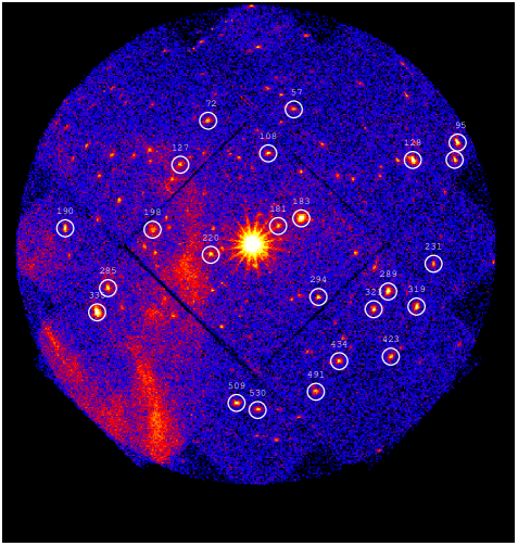
Figure 3: Image of the sky distribution of the 24 brightest sources, in the energy range 0.3–8 keV.

We accumulated the source spectra by selecting only events with PATTERN=0–12 and generated ad hoc response matrices and ancillary files using the SAS tasks rmfgen and arfgen. Before spectral fitting, all spectra were binned with a minimum of 30 counts per bin in order to be able to apply the $\chi^{2}$ minimization technique. In this process, the background count rate was rescaled using the ratio of the source and background areas. Then we fitted the source spectra with four spectral models: power–law, bremsstrahlung, black–body and mekal (i.e. a bremsstrahlung model which includes also the element abundances); in all cases we included also the absorption by the interstellar medium, leaving it as a free parameter. For each emission model, we calculated the 90 % confidence level error on both the hydrogen column density and the temperature/photon–index. In this way we found that 13 sources were best fitted by a power–law model, 2 by a bremsstrahlung model and 2 by a mekal model (Tab. 1). For 6 of the 7 remaining sources, at least two different models provided an acceptable fit with a comparable $\chi_{\nu}^{2}$; finally, for source #127 all the considered models gave unacceptable results.

The spectral parameters were used to compute the sources’ X–ray flux values, to be compared to the optical ones in the framework of the $f_{X}/f_{opt}$ identification tool: for the 23 sources with at least one best–fit model we computed the X–ray flux based on the best–fit values, while for source # 127 we assumed a power–law spectrum with photon–index $\Gamma$ = 1.75 and a galactic hydrogen column density. On the optical side, we considered all the candidate counterparts found within 5” radius X–ray error circles. In order to minimize the effect of the interstellar extinction, we used the $F$ magnitude to calculate the source flux; for the X–ray sources with no counterpart, we used $F$=22 as the optical upper limit.

On the basis of both the spectral fits (N_H and best–fit models) and the X–ray–to–optical flux ratios of the possible counterparts, we can propose a firm classification only for 7 sources, i.e. 6 AGNs and 1 star. For 6 additional sources, the suggested classification (i.e. 4 AGNs and 2 stars) is affected by the best–fit value of the interstellar absorption, which is too low (for AGNs) or too high (for stars) in comparison with the galactic N_H (1.28$\times 10^{21}$ cm^-2). In view of the large errors on the N_H best–fit values, however, we accept the proposed identification.

Table 1: Main characteristics of the 24 brightest sources. The sources are sorted by decreasing count number.

(1)	(2)	(3)	(4)	(5)	(6)	(7)	(8)	(9)	(10)	(11)	(12)
SRC	RA (J2000)	DEC (J2000)	cts	Model	NH	$\Gamma$/kT	$\chi_{\nu}^{2}$	DXO	$F$	$\frac{f_{X}}{f_{F}}$	SUGGESTED
	($hms$)	(∘ ’ ”)			(1021 cm-2)	(-/keV)		(arcsec)	(mag)	(log10)	CLASS
335	12 11 01.37	-52 30 30.6	4229	wabs(pow)	1.8${}^{+0.4}_{-0.4}$	1.95${}^{+0.14}_{-0.13}$	1.03	1.3, 3.1, 3.1, 3.5	20.36, 20.34, 19.35, 19.46	1.39, 1.38, 0.99, 1.03	AGN
183	12 09 41.88	-52 24 56.9	3848	wabs(pow)	0.7${}^{+0.4}_{-0.4}$	1.90${}^{+0.12}_{-0.13}$	1.17	1.5	20.00	0.90	?
128	12 06 58.63	-52 21 26.1	2388	wabs(mekal)	1.3${}^{+0.7}_{-0.6}$	0.61${}^{+0.03}_{-0.03}$	1.42	1.8	10.53	-3.20	STAR
289	12 09 06.02	-52 29 16.8	1499	wabs(pow)	1.3${}^{+0.5}_{-0.5}$	2.00${}^{+0.16}_{-0.17}$	0.77	1.2	19.83	0.57	AGN
95	12 06 41.23	-52 20 25.1	1332	wabs(pow)	0.8${}^{+0.6}_{-0.6}$	2.03${}^{+0.22}_{-0.22}$	1.47	-	$>$22	$>$1.49	AGN (?)
319	12 08 56.96	-52 30 10.1	1109	wabs(brem)	2.1${}^{+2.0}_{-1.2}$	0.33${}^{+0.16}_{-0.13}$	1.40	1.8	13.82	-2.21	STAR (?)
509	12 10 07.06	-52 35 54.2	1056	wabs(pow)	0.8${}^{+0.5}_{-0.6}$	1.78${}^{+0.17}_{-0.19}$	1.25	1.2	19.06	0.29	AGN (?)
323	12 09 13.68	-52 30 19.8	1000	wabs(pow)	0.5${}^{+0.6}_{-0.5}$	1.84${}^{+0.20}_{-0.28}$	0.91	-	$>$22	$>$1.26	?
190	12 11 13.66	-52 25 30.7	984	wabs(brem)	3.1${}^{+2.4}_{-1.3}$	0.30${}^{+0.13}_{-0.11}$	2.35	2.9	14.22	-2.02	?
				wabs(bbody)	1.5${}^{+2.1}_{-0.5}$	0.17${}^{+0.04}_{-0.03}$	2.39	2.9	14.22	-2.02	?
125	12 08 42.36	-52 21 26.6	927	wabs(pow)	0.1${}^{+0.6}_{-0.1}$	1.75${}^{+0.20}_{-0.22}$	1.01	3.1	18.9	0.14	?
530	12 09 58.87	-52 36 19.4	789	wabs(pow)	1.6${}^{+0.9}_{-0.9}$	1.80${}^{+0.24}_{-0.24}$	0.93	2.9, 3.3	17.26, 16.95	-0.52, -0.64	AGN
220	12 10 17.09	-52 27 06.5	769	wabs(brem)	1.8${}^{+1.4}_{-1.0}$	0.40${}^{+0.13}_{-0.13}$	1.01	3.7	15.42	-1.81	STAR (?)
108	12 09 54.74	-52 21 05.4	759	wabs(pow)	1.1${}^{+0.9}_{-1.0}$	2.02${}^{+0.42}_{-0.29}$	0.82	2.4, 4.8	17.27, 18.91	-0.90, -0.24	AGN (?)
72	12 10 18.05	-52 19 09.1	746	wabs(brem)	3.3${}^{+2.8}_{-1.5}$	0.27${}^{+0.12}_{-0.11}$	1.46	0.7	16.56	-1.40	?
				wabs(bbody)	1.5${}^{+2.3}_{-0.6}$	0.17${}^{+0.03}_{-0.05}$	1.45	0.7	16.56	-1.39	?
285	12 10 57.10	-52 29 04.6	738	wabs(mekal)	6.9${}^{+3.4}_{-2.7}$	4.33${}^{+3.84}_{-1.56}$	1.03	1.6, 2.8, 3.7	19.83, 20.43, 18.67	+0.58, +0.82, +0.11	?
				wabs(pow)	7.2${}^{+3.7}_{-2.3}$	1.95${}^{+0.40}_{-0.29}$	1.15	1.6, 2.8, 3.7	19.83, 20.43, 18.67	+0.59, +0.83, +0.12	?
				wabs(bremss)	5.8${}^{+2.7}_{-1.9}$	5.35${}^{+5.45}_{-1.98}$	1.15	1.6, 2.8, 3.7	19.83, 20.43, 18.67	+0.55, +0.79, +0.09	?
434	12 09 27.05	-52 33 25.2	736	wabs(pow)	1.4${}^{+0.8}_{-1.0}$	2.39${}^{+0.40}_{-0.31}$	1.71	-	$>$22	$>$1.11	AGN (?)
491	12 09 36.12	-52 35 14.3	674	wabs(pow)	1.4${}^{+1.0}_{-1.1}$	1.93${}^{+0.37}_{-0.29}$	1.09	-	$>$22	$>$1.22	AGN
423	12 09 06.94	-52 33 08.6	671	wabs(pow)	2.1${}^{+1.2}_{-1.1}$	2.18${}^{+0.30}_{-0.35}$	0.54	1.2	19.72	+0.26	AGN
181	12 09 50.88	-52 25 24.2	669	wabs(pow)	0.8${}^{+0.9}_{-0.8}$	2.15${}^{+0.25}_{-0.28}$	0.91	-	$>$22	$>$0.90	?
				wabs(bremss)	0.0${}^{+0.6}_{-0.0}$	3.20${}^{+1.81}_{-1.20}$	0.97	-	$>$22	$>$0.87	?
				wabs(mekal)	0.0${}^{+0.3}_{-0.0}$	4.02${}^{+1.72}_{-1.01}$	0.99	-	$>$22	$>$0.91	?
294	12 09 35.18	-52 29 36.6	650	wabs(bremss)	2.3${}^{+2.0}_{-1.3}$	3.13${}^{+2.72}_{-1.29}$	0.61	-	$>$22	$>$0.90	?
				wabs(pow)	3.7${}^{+2.8}_{-1.6}$	2.26${}^{+0.59}_{-0.39}$	0.65	-	$>$22	$>$0.93	?
127	12 10 28.87	-52 21 45.7	560	?	-	-	-	1.3	14.93	-1.80	?
198	12 10 39.72	-52 25 36.8	548	wabs(mekal)	3.8${}^{+1.6}_{-1.7}$	0.51${}^{+0.09}_{-0.15}$	1.68	1.6	11.77	-3.39	?
57	12 09 44.83	-52 18 26.8	532	wabs(pow)	1.7${}^{+1.2}_{-1.3}$	1.92${}^{+0.50}_{-0.32}$	1.00	-	$>$22	$>$+1.00	AGN
231	12 08 50.40	-52 27 37.4	490	wabs(bremss)	2.4${}^{+2.2}_{-1.4}$	0.46${}^{+0.23}_{-0.18}$	1.88	1.3	16.25	-1.54	?
				wabs(bbody)	0.6${}^{+2.1}_{-0.6}$	0.23${}^{+0.05}_{-0.06}$	1.92	1.3	16.25	-1.54	?

Key to Table - Col.(1): Source ID number. Col.(2) and (3): source celestial coordinates. Col.(4): source total counts (in the energy range 0.3–8 keV). Col.(5): best–fit emission model(s); the symbol ‘?’ indicates that none of the tested single–component models provided an acceptable fit. Col.(6): best–fit hydrogen column density, with the relevant 90 % confidence level error for two interesting parameters ($\Delta\chi^{2}=4.61$). Col.(7): best–fit photon–index or plasma temperature, in the case of either a power–law or a thermal emission model, respectively; also the relevant 90 % confidence level error for two interesting parameters ($\Delta\chi^{2}=4.61$) is reported. Col.(8): best–fit reduced chi–squared. Col.(9): projected sky distance, from the X–ray position, of the candidate optical counterpart (if any). Col(10): $F$ magnitude of the optical candidate counterpart; we consider $F>$22 if no candidate counterpart is found within a 5” radius X–ray error circle. Col.(11): logarithmic values of the X–ray–to–optical flux ratio; the optical flux is based on the $F$ magnitude; the X–ray flux is based on the best–fit model or, when no model is acceptable, on a power–law spectrum with photon–index $\Gamma$ = 1.75 and hydrogen column density N${}_{\rm H}=1.28\times 10^{21}$ cm^-2, corresponding to the total galactic column density. Col.(12): proposed source classification; the symbol ‘?’ after it means that the reported identification is uncertain, due the N_H value; the only symbol ‘?’ indicates that no classification can be suggested.

4 additional sources (# 190, 72, 198 and 231) are characterized both by a low temperature thermal spectrum and by a low X–ray–to–optical flux ratio, therefore it is probable that they are stars. Unfortunately they have a high N_H value and, in 3 cases, also the emission model is uncertain, therefore the star identification can not be firmly established. For source # 72 this classification would be supported also by the observed light curve (Fig. 4), which shows large but short flares and a flux variability with time–scales of a few hundred seconds.

We note that single component fitting can induce further uncertainty on the N_H estimate. Indeed, stars do show two temperature spectra (actually coronal loop distributions) which, if fitted with a single temperature, would result in an overestimate of the N_H values. AGNs, on the other hand, often have additional soft components which, for a pure power–law fit, would yield too low N_H values. In view of the above uncertainties, we underline that the source classification proposed in Tab. 1 is only tentative.

Figure 4: Light–curve of source #72, with a 1 ksec time binning.

Only the low N_H value prevents to classify as AGNs 3 other sources (# 183, 323 and 125), which are best fitted by a power–law spectrum with photon index $\simeq$2 and have a rather high X–ray–to–optical flux ratio. The smooth variability observed for source # 183, with a time–scale of $\sim 10^{4}$ s (Fig. 5), would also support an AGN identification .

Figure 5: Light–curve of source #183, with a 15 ksec time binning.

For 3 sources with hard spectrum (# 285, 181 and 294) it is not possible to distinguish between a power–law and a high temperature thermal emission model: with all models sources # 285 and 294 show a high N_H value, therefore they are probably extragalactic objects (either AGNs or clusters of galaxies). On the other hand, in all cases source # 181 has a very low best–fit value of N_H, therefore it should be a galactic object, even if its nature can not be established.

Finally, source # 127 has a very unusual spectrum and it will be discussed in detail in Sec. 5.

On the basis of the above results, we conclude that 8 sources over 23 (i.e. $\sim$ 35 %) could belong to the Galaxy. Such a percentage is in agreement with the results obtained by previous ROSAT surveys which showed that the stellar content decreases from $\sim$85% to $\sim$30% moving from the galactic plane to high galactic latitudes (Motch et al. 1997; Zickgraf et al. 2003).

5 Source #127

The X–ray analysis yields 560 counts in the energy band 0.3–8 keV, with a signal–to–noise ratio of 14.64; its count rate in the total energy band is 2.03$\times$10^-3 cts s^-1. The source spectrum cannot be described by a standard single–component emission model (Fig. 6): it is very hard and highly absorbed; moreover, it is also characterized by a feature at $\sim$6 keV, ascribable to Fe emission line.

After the astrometric correction, the resulting X–ray position is $\alpha_{J2000}$=12^h 10^m 28.87^s, $\delta_{J2000}$=-52^∘ 21’ 45.7”. Searching the NED (Nasa/Ipac Extragalactic Database) we found the spiral galaxy ESO 217-G29, located at 1.28” from the X–ray source position. The magnitudes of ESO 217–G29 are $B_{J}=16.74$ and $F=14.93$ and its redshift is $z=0.032$ (Visvanathan & van den Bergh 1992). These parameters, together with the X–ray spectrum and the estimated X–ray–to–optical flux ratio, suggest that source #127 could be an AGN.

The source is located within the region of diffuse emission (Fig. 1), so its spectrum at low energies (E$<$1keV) is polluted by the supernova remnant. Thus we fit the source spectrum only above 1.2 keV. According to the AGN unification model (Antonucci 1993; Mushotzky et al. 1993), the source spectrum $S$ has been described by the model

$S=A_{G}[A_{SP}(R_{W})+A_{T}(PL+R_{C}+GL)]$

where $A_{G}$ is the galactic absorption (1.28$\times$10²¹ cm^-2), $A_{SP}$ is the absorption related to the galaxy hosting the AGN, $R_{W}$ is the warm and optically thin reflection component, $A_{T}$ is the absorption acting on the nuclear emission associated to the torus of dust around the AGN nucleus, $PL$ is the primary power–law modeling the nuclear component, $R_{C}$ is the cold and optically thick reflection component and $GL$ is the Gaussian component that models the Fe line at 6.4 keV. For the $A_{SP}$, $A_{T}$, $R_{C}$ and $GL$ components the redshift value is fixed at $z$=0.032 (Visvanathan & van den Bergh 1992).

Table 2: Best–fit parameters for source # 127, for the optical redshift $z$=0.032 and for its best–fit value $z$=0.057.

Component	Parameter	$z$=0.032 (fix)	$z$=0.057
$A_{SP}$	N${}_{\rm H1}^{a}$	2.26${}_{-1.10}^{+1.42}$	2.39${}_{-1.14}^{+0.81}$
$R_{W}$	$\Gamma$	1.9 (fixed)	1.9 (fixed)
	Flux @ 1 keVb	7.53${}_{-2.78}^{+3.43}$	7.53${}_{-2.63}^{+3.52}$
$A_{T}$	N${}_{\rm H2}^{a}$	75.82${}_{-19.10}^{+25.02}$	82.35${}_{-24.23}^{+18.69}$
$PL$	$\Gamma$	1.9 (fixed)	1.9 (fixed)
	Flux @ 1 keVc	1.93${}_{-0.80}^{+1.37}$	1.98${}_{-0.71}^{+1.51}$
$R_{C}$	$\Gamma$	1.9 (fixed)	1.9 (fixed)
	Flux @ 1 keVc	1.93${}_{-0.80}^{+1.37}$	1.98${}_{-0.71}^{+1.51}$
$GL$	$E_{line}$(keV)	6.4 (fixed)	6.4 (fixed)
	$I_{line}^{d}$	1.26${}_{-1.26}^{+1.81}$	2.33${}_{-1.46}^{+2.42}$
	EQW (eV)	185${}_{-185}^{+265}$	311${}_{-196}^{+322}$
d.o.f.		32	31
$\chi^{2}_{\nu}$		1.143	1.035

^a $10^{22}$ cm^-2

^b $10^{-6}$ ph cm^-2 s^-1 keV^-1

^c $10^{-4}$ ph cm^-2 s^-1 keV^-1

^d $10^{-6}$ ph cm^-2 s^-1

The best–fit parameters, listed in Tab. 2, provide an acceptable fit, yielding $\chi^{2}_{\nu}$=1.143 with 32 d.o.f.; the value of N_H2 implies that the torus around the AGN is Compton–thin. However, this model does not describe satisfactorily the prominent Fe line, since it assigns an energy of 6.2 keV to the line centroid (red solid line in Fig. 6), while in the accumulated spectrum the line is centered around 6.0 keV; moreover, the line significance is marginal.

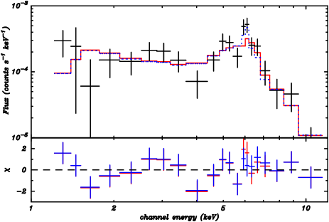
Figure 6: Top: comparison of the unbinned spectrum of source #127 with the best–fit model, in the case of both redshift fixed at $z$=0.032 (red solid line) and of best–fit value $z$=0.057 (blue dotted line). Bottom: data - model residuals (in $\sigma$) for the two above models.

Leaving the $z$ value as a free parameter, we obtain a better fit ($\chi^{2}_{\nu}$=1.035 with 31 d.o.f) for $z=0.057_{-0.016}^{+0.009}$, quite different, although consistent at 2 $\sigma$ level, with the optical value; moreover, the line is significant at 90 % confidence level. Using the F–test, the improvement with respect to the previous fit based on the optical redshift is significant at 95% confidence level. In Tab. 2 we report the best–fit parameters of both fits. As a further check, we applied also the Cash statistics to the XSPEC fit and we obtained the same results: $z$=0.057 and a normalization of 2.26${}_{-1.34}^{+2.14}$ for the iron line. If we compare the source spectrum with the best–fit model (blue dotted line in Fig. 6), we note that the Fe line is modelled more accurately and is centered around 6.0 keV.

The discrepancy between the X–ray and optical redshift values could be explained by the relativistic broadening of the Fe line. Recently, the rest–frame spectra of several sources detected in the XMM–Newton survey of the Lockman hole showed a relativistically broadened iron line (Streblyanska et al. 2005). Owing to the Compton–thin nature of our source, it is possible that we are observing the same phenomenology. This would explain why the best–fit redshift overcomes the cosmological one. We investigated this possibility by modelling the Fe line with a relativistic line ($RL$) from an accretion disc. To this aim we replaced the Gaussian component of our model with either a laor (Laor 1991) or a diskline (Fabian et al. 1989) component , leaving $z$=0.032 for the other components. We fixed the emissivity index $\beta$ to 3 and to -2 for the laor and the diskline case, respectively; moreover, in both cases we fixed the line energy to 6.4 keV and the disc inclination angle $i$ to 30^∘, which is near the best–fit value found by Streblyanska et al. (2005).

In both cases the best–fit model traces rather well the Fe line (Fig. 7) and provides an acceptable fit, yielding $\chi^{2}_{\nu}$=1.034 and 1.087 for the laor and the diskline component, respectively. For both models we find that the relativistic component is significant at 90 % confidence level. However, the disc inner and outer radii values are too small (i.e. a few $R_{g}$) and their difference is not significant. Moreover, only for the laor component the line EQW is comparable to the value of $\sim$0.4 keV found by Streblyanska et al. (2005), while it is significantly larger ($\sim$ 1 keV) for the diskline. Since these parameters are affected by large errors, due the low count statistics, we conclude that the iron line position can be reconciled with the redshift of the proposed optical counterpart ESO 217-G29.

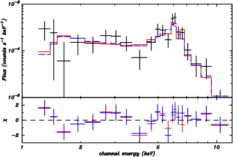
Figure 7: Top: comparison of the unbinned spectrum of source #127 with the best–fit model and $z$=0.032, in the case of both a laor (red solid line) and a diskline (blue dotted line) model for the Fe line. Bottom: data - model residuals (in $\sigma$) for the two above models.

The 2–10 keV unabsorbed flux of the primary nuclear component is 5.79${}_{-2.40}^{+4.11}\times 10^{-13}$ erg cm^-2 s^-1 (calculated with XSPEC). Such a flux value, together with the optical magnitude, implies that $f_{X}/f_{opt}$=0.41, i.e. well within the AGN range (Krautter et al. 1999). The X–ray luminosity of the source in the 2–10 keV energy band, corrected by the absorption and with the redshift at 0.032, is 2.59${}_{-1.07}^{+1.84}\times 10^{42}$ erg s^-1, corresponding to a low luminosity Seyfert galaxy.

Thus, the X–ray spectrum, together with the best–fit value of N_H2 and the nature of the optical candidate counterpart led us to propose that source #127 could be a new, low–luminosity Seyfert–2 galaxy discovered serendipitously in our field.

6 Summary and conclusions

The longest XMM–Newton observation at low galactic latitude yielded a sample of 135 sources between 0.5 and 2 keV and of 89 sources between 2 and 10 keV, with limiting fluxes of $1.3\times 10^{-15}$ and $3.4\times 10^{-15}$ erg cm^-2 s^-1, respectively. The log$N$–log$S$ distribution of the hard sources is comparable to that measured at high galactic latitudes, thus suggesting that it is dominated by extragalactic sources. On the other hand, at low fluxes the distribution of the soft sources shows an excess above both the Galactic Plane and the high–latitude distributions: we consider this result as a strong indication that we observed a sample of both galactic and extragalactic sources.

We analysed the 24 brightest sources and proposed an identification for $\sim$ 80 % of them. Moreover, the detailed spectral investigation of one unidentified source, characterized by a highly absorbed spectrum and an evident Fe emission line, led us to classify it as a new Seyfert–2 galaxy.

The full X–ray characterization of all the sources, as well as their classification, based on ad hoc optical observations, will be discussed in future papers.