Gamma-Ray Polarimetry of Two X-Class Solar Flares

Abstract

We have performed the first polarimetry of solar flare emission at $\gamma$-ray energies (0.2–1 MeV). These observations were performed with the Reuven Ramaty High Energy Solar Spectroscopic Imager (RHESSI) for two large flares: the GOES X4.8-class solar flare of 2002 July 23, and the X17-class flare of 2003 October 28. We have marginal polarization detections in both flares, at levels of 21 $\pm$ 9% and -11 $\pm$ 5% respectively. These measurements significantly constrain the levels and directions of solar flare $\gamma$-ray polarization, and begin to probe the underlying electron distributions.

1 Introduction

It has been recognized for nearly four decades that X-ray polarization could serve as a strong diagnostic of electron beaming in solar flares (Korchak, 1967; Elwert, 1968), which is crucial for understanding the underlying particle acceleration process. While the X-ray spectral measurements are relatively insensitive to the underlying electron distributions, the X-ray polarization is predicted to vary from a few percent for nearly isotropic electron distributions, to 20–25% for highly beamed distributions (Haug, 1972; Brown, 1972; Langer & Petrosian, 1977; Bai & Ramaty, 1978; Leach & Petrosian, 1983; Zharakova, Brown, & Syniavskii, 1995; Charikov, Guzman, & Kudryavstev, 1996). The direction of the polarization vector – whether parallel or perpendicular to the projected magnetic field – will depend on whether the electrons are primarily beamed along the magnetic field lines (small pitch angle) or perpendicular (large pitch angle). In addition, the degree and direction of polarization will be a function of the the viewing angle to the flare, i.e. radial position on the solar disk. Therefore, in order to constrain electron beaming models, we would ultimately like to measure the degree and direction of linear polarization for many flares, covering the full range of viewing angles over the solar disk.

Solar X-ray polarization observations have historically proved difficult [see Chanan, Emslie, & Novick (1988); McConnell et al. (2004) for overviews]. All of these measurements were performed at energies below 20 keV (Tindo et al., 1970; Nakada et al., 1974; Tindo et al., 1976; Tramiel, Chanan, & Novick, 1984), where the emission is strongly contaminated by thermal emission, significantly complicating interpretation of the measurements. These observations and subsequent analyses have lead to the general conclusion that the best energy range for studying flare polarization is $>$50 keV (Chanan, Emslie, & Novick, 1988). At energies above 1 MeV, flare emission is dominated by nuclear lines which are expected to be unpolarized; therefore, the best energy band for studying solar flare polarization is 50 keV – 1 MeV (Lei, Dean & Hills, 1997; Chanan, Emslie, & Novick, 1988). To date, there have been no attempts to study the $\gamma$-ray polarization, and theoretical predictions above 200 keV are limited (Haug, 1972; Langer & Petrosian, 1977; Bai & Ramaty, 1978). Studies are currently being performed in the 50–100 keV band with RHESSI using an extension of the techniques used previously in the lower energy observations (McConnell et al., 2002), with results in preparation (McConnell, private communication). This paper is the first attempt to measure solar flare polarization above 200 keV, where the thermal emission is truly negligible.

While not primarily designed as a polarimeter, RHESSI is sensitive to polarization in both the 20–100 keV band, and the 0.2–1 MeV band. A passive Be block was added to the RHESSI focal plane in order to detect polarization in the hard X-ray range (20–100 keV) (McConnell et al., 2002). At higher energies ($>$ 200 keV), Compton scattering of photons between the detectors themselves can be used to measure polarization. This technique has been used with RHESSI data to search for polarization from $\gamma$-ray burst GRB 021206 (Coburn & Boggs, 2003; Wigger et al., 2004). While the results for this GRB remain controversial, the work on this burst confirms the sensitivity of RHESSI to polarization for bright $\gamma$-ray events. The factors that made GRB 021206 so difficult to analyze (short duration, rapid variability, off-axis location, relatively small number of counts, telemetry decimation) go away for these solar flares, simplifying the analysis. Indeed, given the large number of flare photons, we have implemented an analysis method with much stricter data selection than implemented in our analysis of GRB 021206 (Coburn & Boggs, 2003) in order to address the concerns raised by subsequent analysis (Wigger et al., 2004).

We will first give an overview of the RHESSI instrument and discuss how it can be used to measure $\gamma$-ray polarization. Next, we discuss in detail our methods used for this analysis. Finally, we present a brief discussion of the scientific implications of these observations.

2 RHESSI Instrument

RHESSI has an array of nine coaxial germanium detectors, designed to perform detailed spectroscopic imaging of X-ray and $\gamma$-ray emission (3 keV – 17 MeV) from solar flares (Lin et al., 2002). RHESSI imaging is performed by two arrays of opaque 1-D grids, separated by 1.5 m, and co-aligned with the nine detectors (Zehnder et al., 2003). As the RHESSI spacecraft rotates (4-s period, axis aligned with the Sun) these grids modulate the count rate in the detectors, allowing imaging through rotational modulation collimator techniques (Hurford et al., 2002). Thus, RHESSI has high angular resolution (2.6$\,{}^{\prime\prime}$) in the 1^∘ field of view of its optics. In addition, RHESSI sends down the energy and timing information for each photon, allowing detailed timing measurements.

2.1 RHESSI Spectrometer

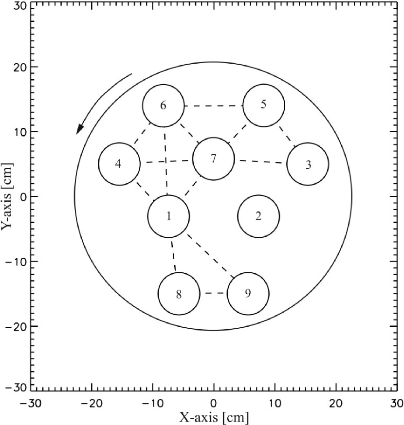
Figure 1: Configuration of the nine RHESSI detectors in the plane of the spectrometer as viewed from the front of the spacecraft, which rotates in the direction indicated with a 4-s period. The dashed lines represent detector-detector coincidence paths among the neighboring rear segments used in this analysis. Detector #2 was not used (see text).

The heart of the RHESSI instrument is the array of nine coaxial germanium detectors, 7.1-cm diameter, 8.5-cm height each (Smith et al., 2002). The detectors are arranged in the spectrometer as shown in Fig. 1. RHESSI performs its imaging by photon timing, not positioning, so there is no spatial information for interactions within a detector segment – just energy and timing information. The detectors are designed to be electrically “segmented” into two monolithic sections, so that the front segments ($\sim$1.5-cm thickness) perform as separate detectors, with separate electronics, from the rear segments ($\sim$7.0-cm thick). RHESSI detectors are segmented in order to optimize performance over its broad energy band: solar X-ray and hard X-ray photons ($<$100 keV) will preferentially stop in the “fronts”, while $\gamma$-rays ($>$100 keV) will preferentially interact in the “rears”. Given the overwhelming X-ray and hard X-ray fluxes from large flares, the fronts both measure the low energy emission, as well as shield the rears from these overwhelming count rates, for minimal deadtime to the $\gamma$-ray emission. Detector #2 initially failed to segment after the launch of RHESSI, and therefore acts as a single detector covering the whole front and rear volume at the times of these observations. The fronts have a typical threshold of 2.7 keV, and a spectral resolution of roughly 1 keV at 94 keV. The rears have a typical threshold of 20 keV, and a spectral resolution of 3 keV at 1.117 MeV. When an interaction occurs in a rear segment, there is a deadtime of 8–9 $\mu$s before another interaction can be measured in the same rear.

For our solar flare polarization analysis, we are using only the rears in order to avoid the overwhelming flux in the fronts. By including the front segments during these flares, our livetime to real scatter events goes nearly to zero, and our coincidence events are dominated by chance coincidences. In this analysis the fronts are treated effectively as passive material. For these same reasons, we exclude detector #2 from this analysis. Our polarization analysis utilizes the rear segments of detectors #[1,3,4,5,6,7,8,9]. In order to maximize the signal-to-noise, we include only scatters that occur between adjacent detector pairs since these will dominate the real scatter events, and minimize chance coincidences. The possible scatter paths included in our analysis are sketched in Fig. 1.

2.2 RHESSI Data

RHESSI sends down data for each individual interaction in its detectors (“photon-mode”). Here we are careful to differentiate “interactions” from “photons.” For most events in the RHESSI instrument these are one and the same. We are interested, however, in the subset of photon events which have interactions in multiple detectors. We have tried to be consistent here in our use of these two terms. For each interaction, there are three primary pieces of information: interaction time, interaction energy, and detector segment identification. Each interaction is tagged with a time resolution of 1 “binary microsecond” (1 b$\mu$s = 2^-20 s), and $\sim$0.3-keV energy sampling.

RHESSI does not have detector-detector coincidence electronics, so coincidences have to be determined by comparing the times of individual interactions. Whether any given interaction is a photon that interacted in a single detector, or is part of a coincident photon scattering event, must be determined by analysis of the interaction times. Between the rear segments we use in this analysis, we require coincidences to have $\Delta$t = 0 b$\mu$s (i.e., within one RHESSI time resolution unit). This criteria is discussed in detail below.

RHESSI often enters a “decimation” mode where only a fraction of the events in the rears will be stored for energies below $\sim$380 keV, typically $\frac{1}{6}$ to $\frac{1}{4}$, which is designed to save on-board memory during periods of high background. This decimation mode can significantly complicate polarization analysis (Wigger et al., 2004), so we have chosen only flare periods and background periods when RHESSI was not decimating in the rears.

2.3 RHESSI $\gamma$-ray Polarimetry

RHESSI is not designed to be a Compton $\gamma$-ray polarimeter; however, several aspects of its design make it sensitive to polarization. In the $\gamma$-ray range of 0.15–10 MeV, the dominant photon interaction in the RHESSI detectors is Compton scattering — yet most photons are eventually photabsorbed in the same detector in which they initially scattered. A small fraction of incident photons will undergo a single scatter in one detector before being scattered and/or photoabsorbed in a second separate detector. These scattered-photon events are sensitive to the incident $\gamma$-ray polarization since linearly polarized $\gamma$-rays preferentially scatter in azimuthal directions perpendicular to their polarization vector. In RHESSI, this scattering property can be used to measure the intrinsic polarization of solar flares.

The sensitivity of a Compton polarimeter is determined by its effective area to scatter events, and the average value of the polarimetric modulation factor, $\mu$, which is the maximum variation in azimuthal scattering probability for polarized photons (Novick, 1975; Lei, Dean & Hills, 1997). This factor is given by:

$$\mu(\theta,E_{\gamma})=\frac{d\sigma_{\perp}-d\sigma_{\parallel}}{d\sigma_{\perp}+d\sigma_{\parallel}},$$ (1)

where $d\sigma_{\perp}$, $d\sigma_{\parallel}$ are the Klein-Nishina differential cross sections for Compton scattering perpendicular and parallel to the polarization direction, respectively, which is a function of the incident photon energy $E_{\gamma}$, and the Compton scatter angle $\theta$ between the incident-photon direction and the scattered-photon direction. For a source of count rate $S$ and fractional polarization $\Pi_{s}$, the expected azimuthal scatter angle distribution (ASAD) is given by:

$$\frac{\partial S}{\partial\phi}=(\frac{S}{2\pi})[1-\mu_{m}\Pi_{s}\cos{2(\phi-\eta)}],$$ (2)

where $\phi$ is the azimuthal scatter angle, $\eta$ is the direction of the polarization vector, and $\mu_{m}$ is the average value of the polarimetric modulation factor for the instrument. While RHESSI has a small effective area for events that scatter between detectors due to its large-volume detectors (photons have a small probability of escaping a detector after their first scatter), it has a relatively large modulation factor in the 0.2–1 MeV range, $\mu_{m}\sim 0.32$, as determined by Monte Carlo simulations described below.

RHESSI also has the advantage of rotating around its focal axis (centered on the Sun) with a 4-s period. Rotation averages out the effects of scattering asymmetries in the detectors and passive materials that could be mistaken for a modulation. Sources that vary on timescales longer than the rotation period will be relatively insensitive to the systematic uncertainties that typically plague polarization measurements. The photon scatters between any pair of detectors will modulate twice per rotation due to a polarized component. We note that this modulation is orders of magnitude slower than modulations introduced by the imaging grids (Hurford et al., 2002).

Finally, while the RHESSI detectors have no positioning sensitivity, they are relatively loosely grouped on the spacecraft, allowing the azimuthal angle for a given scatter to be determined to within $\Delta\phi\simeq$ 13^∘ r.m.s., as determined by the diameter of the detectors and their typical spacing (Fig. 1). This angular uncertainty will decrease potential modulations by a factor of 0.95, which is included in our calculated modulation factor.

3 Observations

For this analysis we chose two of the brightest $\gamma$-ray flares seen by RHESSI, both with strong emission above 0.2 MeV. The 2002 July 23 flare was chosen specifically due to the large volume of RHESSI imaging and spectroscopy analysis performed on this flare. The 2003 October 28 flare was chosen both due to its strong $\gamma$-ray emission, and because it is one of the few $\gamma$-ray flares RHESSI has observed toward the center of the solar disk, providing a smaller viewing angle relative to solar vertical than the 2002 July 23 flare. For a given flare we had two criteria for the time interval analyzed, both designed to maximize signal-to-noise. First, we required the 0.2–1 MeV flare photon rate to be greater than the background photon rate. Second, we required the rate of real photon-scatter coincidences to be larger than the chance coincidence rate (Sec. 4.5).

3.1 23 July 2002

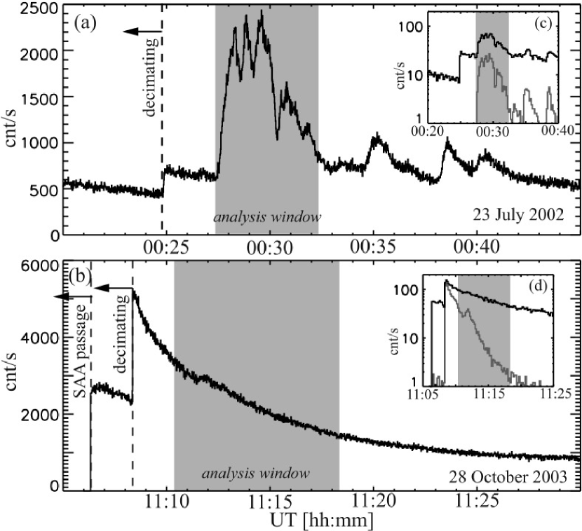
Figure 2: Lightcurves of 0.2-1 MeV single events in the RHESSI rear segments for (a) the 23 July 2002 flare, and (b) the 28 October 2003 flare. The insets (c) and (d) show the total coincidence rates (dark line) and the chance coincidence rates (light line) among the rears during the flare. The periods we used in this analysis are shown in grey.

On 23 July 2002 an X4.8-class flare was observed by RHESSI through its initial rise (00:18–00:27 UT), impulsive phase (00:27–00:43 UT), and much of its subsequent decay [Lin et al. (2003), and references therein]. The uncorrected 0.2–1 MeV lightcurve for the RHESSI rear detectors is shown in Fig. 2a. To be clear, these are the single interactions in the rear segments. From the lightcurve the period when RHESSI is decimating in the rears is obvious. For this analysis, we selected the time interval UT 00:27:20–00:32:20 to study for polarization. This interval avoids decimation periods, as well as selects a period when the flare dominates the count rate. The emission from this flare originated at S13^∘, E72^∘, near the limb of the solar disk, resulting in a viewing angle of 73^∘.

3.2 28 October 2003

On 28 October 2003 the tail of the impulsive phase of an X17-class flare was observed by RHESSI at 11:06 UT, just as the satellite was emerging from the South Atlantic Anomaly (SAA), through which the detectors are turned off. Therefore, RHESSI missed much of the initial rise of this flare. In addition, the decay phase was cut off due to Earth occultation of the sun during the RHESSI orbit. Despite these limitations, which have minimized the standard RHESSI analysis of this flare compared to the 23 July 2002 flare, we chose this flare for polarization analysis for two reasons. First, it is very bright in the $\gamma$-ray range. Second, this is the strongest flare RHESSI has seen near the center of the solar disk (S17^∘, E9^∘), with a viewing angle of 19^∘. The uncorrected 0.2–1 MeV lightcurve for the RHESSI rear detectors is shown in Fig. 2b. For this analysis, we selected the time interval UT 11:10:22–11:18:22 to study for polarization. This is offset from the peak measured $\gamma$-ray rates by approximately two minutes; however, during the peak of the emission the count rate is high enough that the livetime for measuring scattered photons in the rear segments is near zero (Sec. 4.5).

4 Analysis Method

The ultimate goal of this analysis is to study the azimuthal scatter angle distribution (ASAD) for photons that scatter between RHESSI detectors, as this distribution is projected on the solar disk, i.e. corrected for the rotation of the spacecraft. Therefore, for each scatter event we need to determine the angle of the scatter in the plane of the instrument, as determined by the center-to-center direction of the two detectors involved, as well as the instantaneous rotation angle of the RHESSI spacecraft. In our plots of the ASAD, 0^∘ is defined as east in solar coordinates, and the azimuthal angle is measured clockwise relative to this direction (i.e., 90^∘ is solar north).

4.1 ASAD Derivation

Here we present a detailed description of our analysis method for deriving the ASAD for each flare. All manipulations of the raw photon data, to the point of binning the scatter directions into an ASAD, are handled with standard RHESSI software under the SolarSoft (SSW) system:

Step 1. Read in all RHESSI interactions during the defined time interval.

By default, we always begin with all the interactions that occurred within the RHESSI detectors during our time interval of interest.

Step 2. Reject all events which do not occur among the rear segments.

By rejecting all of the other interactions, we are effectively treating the front segments as passive shielding from low-energy photons. Thus, we are including some photons in our ASAD which scattered first in a front segment, effectively depolarizing the photon before subsequently scattering between rears. These events are properly included in our calculations of the modulation factor (Sec. 4.6), treated as a background component which decreases the measured modulation. The same is true of all passive material in the spacecraft.

Step 3. Apply the energy calibration.

Use standard RHESSI software to perform a careful energy calibration and determine the energy of each interaction.

Step 4. Reject all interactions $<$10 keV.

These events are predominantly noise triggers in the rear detectors.

Step 5. Determine rear-rear coincidences, reject other interactions.

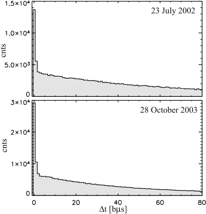
Figure 3: Distribution of waiting times ($\Delta$t) between single interactions for each flare. The peak at $\Delta$t = 0 b$\mu$s is a clear signal of the true photon-scatter coincidences. The underlying continuum is due to chance coincidences. There are some true scatter coincidences in the $\Delta$t = 1 b$\mu$s bin, but we have excluded them to maximize the signal-to-noise.

Coincidences are determined (Sec. 4.2, Fig. 3) by finding interactions in two separate rears with identical time tags ($\Delta$t = 0 b$\mu$s), while requiring that there were no other interactions within 4 b$\mu$s in any rear, either before or after this coincident pair. All non-coincident events are rejected at this point.

Step 6. Reject any coincident pair where either interaction is $<$30 keV.

This step is designed primarily to reject chance coincidences due to higher background from flare photons at low energies. Relatively few photons above 0.2 MeV will lose $<$30 keV in Compton scatter interactions. In practice, no photons at these low energies can directly reach the rear segments through the fronts, so these events are dominated by low energy photons which have scattered off the spacecraft or Earth’s atmosphere and into the rears.

Step 7. Reject any coincident pair whose combined “photon” energy does not lie in the 0.2–1 MeV range.

This is the optimal photon energy band for Compton $\gamma$-ray polarimetry with RHESSI for solar flares. Below 0.2 MeV, few photons have enough energy to scatter out of one detector and into another. Above 1 MeV, the solar flare emission is dominated by nuclear line emission. We also reject photons within a 20-keV band centered on the 0.511-MeV electron-positron annihilation line as well. (We present results in the 0.2–0.4 MeV and 0.4–1 MeV bands separately in Sec. 4.7.4.)

Step 8. Reject coincident pairs inconsistent with Compton scatter kinematics.

The most reliable coincident events for studying polarization will be those that scatter a single time in one detector, and then are completely absorbed (in one or more interactions) in a second detector. Since RHESSI does not resolve the photon interactions within a detector, we can not determine this absolutely for any coincident pair. But we can check that the energies recorded in the two detectors are consistent with a Compton scatter of a photon with total initial energy given by the sum of the interactions in the two detectors. In addition, we make a more stringent cut at this point. Since real photon scatters between the detectors are likely large-angle Compton scatters, which are the scatters most sensitive to polarization, we require that the energies measured in the two detectors be consistent with a Compton scatter angle in the range 45^∘–135^∘. These cuts help reject chance coincidences and photons with incomplete energy depositions, as well as forward-scatter and back-scatter events that are least sensitive to polarization (but see Sec. 4.7.3).

Since we only measure the energies in the two detectors for coincident events, there is not enough redundant information to verify that the photon was fully absorbed, and that the scatter angle lies within the optimal range. However, we can verify that the energies are consistent with these conditions. To be explicit, we start with the assumption that the photon was fully deposited, i.e. the initial photon energy is equal to the sum of the two measured energies. Then we check both possible interaction orderings to verify whether either one is consistent with a photon, of that assumed initial energy, scattering between the two detectors with a a Compton scatter angle in the range 45^∘–135^∘. If neither interaction order is consistent with this Compton scatter angle range, we reject the event – these are likely to be photons that had Compton scatter angles outside the optimal range, or photons that were not full stopped in the detectors. If one or both of the potential interaction orderings are consistent with a Compton scatter angle in this optimal range, we assume the event is good and keep it in the analysis.

Step 9. Determine the most-likely direction of scatter between the two detectors, in the instrument frame of reference (FOR).

From the same Compton kinematic analysis in Step 8, we can determine the most-likely order in which the photon scattered between the detectors. This determines the photon scatter direction in the instrument FOR, which we take to be the center-to-center direction between the detector pairs. We note that the Compton scatter information does not help to constrain this azimuthal scatter angle direction (we have to take the direction as between the two detector centers); however, this information helps determine the order in which the photon scattered between the detectors. From our analysis in Step 8, if only one potential interaction ordering is consistent with the Compton kinematic cuts, we assume that ordering is the correct one. If both potential interaction orderings are consistent with the Kinematic cuts, then we assume that the interaction with the smaller energy deposition was the initial scatter. This assumption is consistent the Compton scattering having a higher cross section for scattering in the forward direction, and we confirmed that this choice of interaction ordering has a higher probability from the Monte Carlo simulations. (Note, however, that since polarization modulations are 180^∘-symmetric, the choice of this interaction order should not affect the final results, as long as a consistent choice is made for these ambiguous cases.)

Step 10. Correct for the spacecraft rotation.

Using standard RHESSI analysis software, we determine the rotation angle of the spacecraft (relative to fixed solar coordinates) at the instant of each coincident event. Then the scatter direction in the instrument FOR for each interaction is corrected to the scatter direction relative to the solar disk.

Step 11. Create the ASAD.

The individual scatter directions are binned to create an ASAD for the time interval. We bin the events in 24 bins, 15^∘ each, covering a full 360^∘.

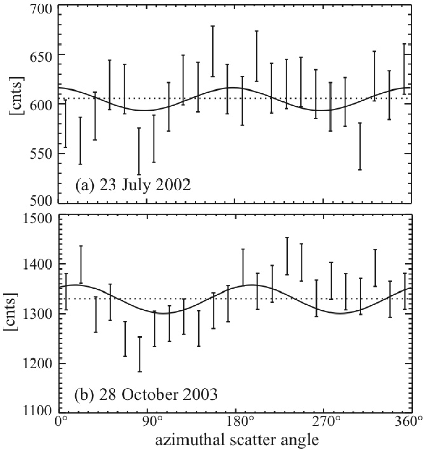
Figure 4: The 0.2-1 MeV raw flare ASADs (no background subtracted) for (a) the 2002 July 23 flare, and (b) the 2003 October 28 flare. Averages are shown for each ASAD (dotted line).

Fig. 4 shows the raw flare ASAD for 0.2–1 MeV scatter events for both the 23 July 2002 flare and the 28 October 2003 flares. These raw distributions are really the sum of three components: the true scattered photons from the flare, scattered photons from the background, and chance coincidences between detectors. In addition, there is another background component which includes photons which first scatter in the passive spacecraft material before subsequently scattering between the rears; however, this component is treated separately through the modulation factor (Sec. 4.6). An unpolarized signal should be flat, while polarization should manifest itself in this ASAD as a sinusoidal component with a period of 180^∘. Before we search for a modulation, we need to determine the background and chance coincidence distributions, and the modulation factor for the observations.

4.2 Coincidence Window

As noted above, RHESSI does not have detector-coincidence electronics; therefore, photon scatter events between detectors have to be determined by the interaction timing information. In order to determine the detector coincidence timing window, as well as the rate of chance coincidences, we perform an identical analysis to the steps identified above, except at Step 5 we record the time difference between every pair of interactions adjacent in the event list. These time differences are binned by the RHESSI time resolution, 1 b$\mu$s. The distribution of time differences for our two flare intervals are plotted in Fig. 3. The real scatter coincidences (both flare and background photons) show up as a strong peak in this distribution at $\Delta$t = 0 b$\mu$s. The underlying continuum is the chance coincidence distribution, which is expected to be an exponential distribution with a time constant given by the average time between interactions (or, the inverse of the interaction rate). This distribution allows us to determine the coincidence window for true photon scatter events ($\Delta$t = 0 b$\mu$s) and the underlying rate of chance coincidences within this window. We note that the number of events in the coincidence window for both data sets is very close to the number of events in the ASAD derived through the steps above. (Given the slight differences required in deriving the curves, we expect the peak in the time-difference distribution to be slightly lower.)

4.3 Chance Coincidences

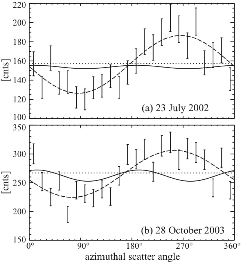
Figure 5: The 0.2-1 MeV chance-coincidence ASADs ($\Delta$t = 4 b$\mu$s) for (a) the 2002 July 23 flare, and (b) the 2003 October 28 flare. Averages are shown for each ASAD (dotted line), as well as the best-fit 360^∘ sinusoidal fits (dashed line), and the best-fit modulations (solid line). The 360^∘ component appears to be a systematic instrumental effect associated with these chance coincidences, and subtracts away in our final flare ASAD.

In order to subtract the chance-coincidence ASAD from the raw distribution shown in Fig. 4, we follow the same steps as outlined above, except instead of requiring the interactions to occur with $\Delta$t = 0 b$\mu$s, we require the time difference between the interactions to be $\Delta$t = 4 b$\mu$s. This creates a scatter angle distribution of interactions that are purely chance coincidences, with the number of chance coincidences nearly identical to the number within our raw flare ASAD. The chance coincidence ASADs are shown in Fig. 5.

For unpolarized signals, we expect all the ASADs to be flat. A polarized component will show up as a sinusoidal modulation on top of this flat distribution with a period of 180^∘, since Compton scattering is symmetric around the polarization axis. We do not expect a sinusoidal component in this distribution with a 360^∘ period; however, these components show up quite clearly in both the raw flare ASADs (Fig. 4) and the chance-coincidence ASADs (Fig. 5). Indeed, the 360^∘ component appears to be an instrumental effect due solely to the chance coincidences, and disappears from the flare ASAD when we subtract off the chance-coincidence component. We do not understand the origin of this 360^∘ period component, but it appears to be a systematic instrumental effect arising from the chance coincidences, and subtracts away with this component.

In Sec. 4.7.3 we discuss how we used these chance coincidence ASADs to verify that the chance coincidences are consistent with zero polarization, as expected.

4.4 Background Scatters

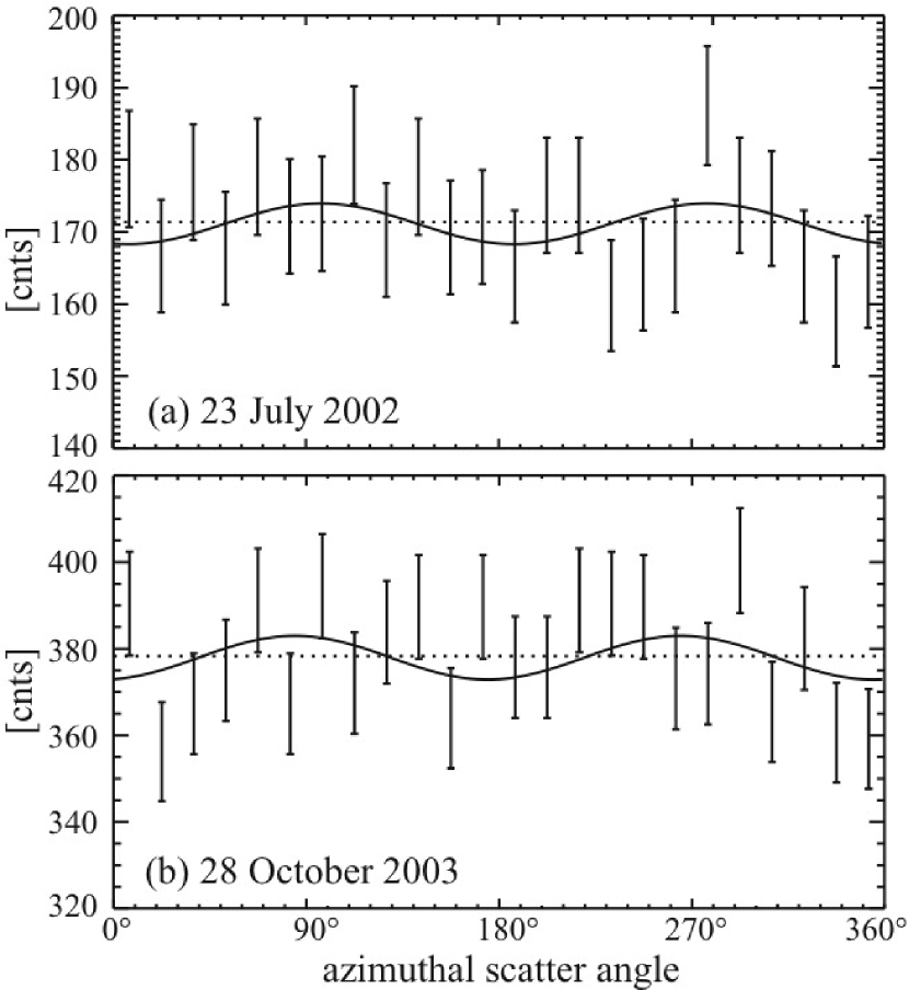
Figure 6: The 0.2-1 MeV average background ASADs (taken during orbits immediately before and after the flares) for (a) the 2002 July 23 flare, and (b) the 2003 October 28 flare. Averages are shown for each ASAD (dotted line), as well as the best-fit modulations (solid line).

Since the RHESSI detectors are unshielded, they are subject to a constant background of true cosmic and atmospheric photons, some fraction of which scatter between the detectors identically to the flare photons. To determine the background component to our scatter angle distribution, we identify two background time periods for each flare identical in length to our flare time intervals: one background period during the orbit before the flare, and one interval during the orbit following the flare. These time intervals are defined in Table 1. The average background ASADs are shown in Fig. 6, scaled by by the scatter livetimes discussed in Sec. 4.5.

The difference in the scatter-coincidence rates for the two background periods we chose for each flare are larger than anticipated from purely statistical fluctuations, which is expected since the RHESSI background varies significantly on orbital timescales. We characterize our systematic uncertainty on the background scatter rate as half of the difference between the two backgrounds selected for each flare. This systematic uncertainty dominates the overall uncertainty on our average background-subtracted scatter rate during the flare.

The average background ASADs show no significant signs of the 360^∘ period components, likely due to the small number of chance coincidences during the background intervals. The background distributions also do not show any significant 180^∘ modulations. In Sec. 4.7.3 we discuss how we used these average background ASADs to verify that the background events are consistent with zero polarization, as expected.

4.5 Scatter Livetime

In Figs. 2a & 2b we showed the 0.2–1 MeV single interaction rates in the rears. In Figs. 2c & 2d we show the total coincidence rates among the rears for all the detector pairs shown in Fig. 1, and the chance coincidence rates among the same pairs as determined by the method in Sec. 4.3. As can be seen in Figs. 2c & 2d, the chance coincidence rates do not scale linearly with the single interaction rates. Indeed, we see that when the rates get high enough the coincident events are dominated by the chance coincidences, with the number of real scatter events dropping. The system responds as if there is an effective livetime to real scatter events, which drops to zero if the event rate is high enough.

We note that this is a separate problem from determining the ratio of real scatter events to chance coincidence events, which is straightforward to determine from the peak in Fig. 3 at $\Delta$t = 0 b$\mu$s relative to the underlying continuum.

This effective scatter livetime and saturation at high count rates affects our analysis in two ways. First, in order to maximize our real scatter signal and limit the chance coincidence background, we select only time intervals where the photon scatter rate is greater than the chance coincidence rate, as determined by making time-resolved versions of Fig. 3. This criteria did not affect the 2002 July 23 analysis, but explains why our 2003 October 28 flare analysis window is offset several minutes after the peak single interaction count rate in the rears.

The second effect on the analysis is determination of this effective scatter livetime. Since we derive the background ASADs from off-flare time intervals, direct subtraction of the average background ASAD will over subtract background from the flare ASAD since the real background scatter rate is reduced by the effective scatter livetime during the time of the flare. Therefore, to properly subtract this component our average background ASADs must be corrected by this effective scatter livetime before subtraction from the raw flare ASADs. (The average background ASADs shown in Fig. 6 have already been corrected by these livetime factors.)

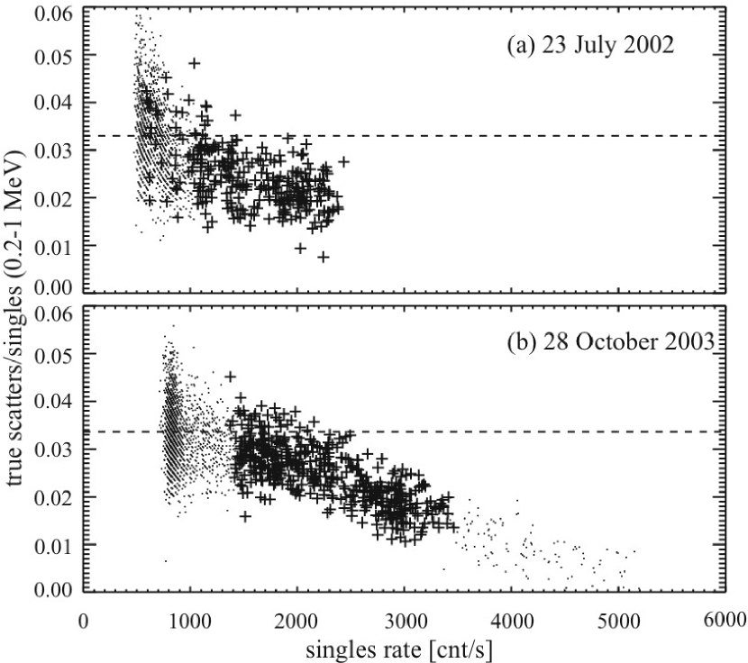
Figure 7: The ratio of 0.2-1 MeV true photon scatters to singles count rate, as a function of the singes count rate. The dots show all data around the time of the flare, while the crosses are from the times taken for the polarization analysis. For a constant scatter livetime we would expect this curve to be flat – the drop at higher count rates show a corresponding drop in the effective scatter livetime. By comparing the average of this ratio for times used in our analysis (crosses) to the average at low count rates (dashed line) we can directly measure the effective scatter livetimes for these analysis periods.

For our flare periods, estimating the scatter livetime is straightforward if we make the reasonable assumption that background photon scatters and flare photon scatters are suppressed by the same effective livetime during the flare. These scatter livetimes were determined by plotting the ratio of true scatter events (determined by time-resolved versions of Fig. 3) to single events, as a function of the overall singles event rate (Fig. 7). If there were no effective deadtime to scatter events, we would expect these plots to be flat; however, we can clearly see a roll-off in this ratio at high count rates. By determining the average ratio at low count rates, and the average ratio for our observation period, we can take their ratio as our effective scatter livetime (Fig. 7). For our analysis periods listed in Table 1, we estimate the fractional scatter livetimes to be 0.73$\pm$0.01 for the 2002 July 23 flare, and 0.74$\pm$0.01 for the 2003 October 28 flare.

4.6 Modulation Factor

Before we can determine the intrinsic polarization of the flares, we need to estimate the modulation factor for the RHESSI instrument. The modulation factor will depend on a number of factors including the detector geometries, the spectral shape in the 0.2–1 MeV range, and the energy and Compton kinematics cuts that we perform in deriving the ASAD.

Photons which first scatter in the passive material of the spacecraft will be effectively depolarized before subsequently scattering between rears. While these are effectively a background component in the flare ASAD, they are not a component that we can identify and subtract as a background. Instead, these events must be properly included in our calculations of the modulation factor, treated as a background component which will decrease measured modulations, and therefore the modulation factor. These events have been properly included and accounted for in our calculations of the modulation factor.

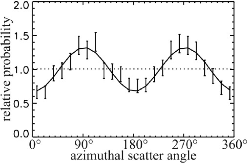
Figure 8: The simulated ASAD for 100% polarized solar photons in the 0.2–1 MeV range, assuming an input spectrum of the form measured for the 23 July 2002 flare (Sec. 4.6). The modulation on this distribution corresponds to an instrumental modulation factor for RHESSI of $\mu_{m}$ = 0.32$\pm$0.03.

In order to determine this modulation factor, we utilized a detailed RHESSI mass model, implemented for the MGEANT interface of the CERN GEANT Monte Carlo package (Sturner et al., 2000), with the GLEPS package which includes $\gamma$-ray polarization (McConnell et al., 2002). This mass model was developed to study the RHESSI background components (Wunderer et al., 2004). As an input spectrum, we chose the best-fit spectral distribution determined for the 23 July 2002 flare, which corresponds to a broken power law with an index break from 2.77 to 2.23 at 617 keV (Smith et al., 2003). We verified that this modulation factor does not significantly change for pure power law spectra with spectral indices ranging between 2 and 3, which encompasses our broken power law spectrum. We performed the same data cuts on the simulated interactions that we performed on the real interactions. By simulating 100% polarized photons, we can measure the modulation factor directly from the simulated ASAD, shown in Fig. 8, to derive $\mu_{m}$ = 0.32$\pm$0.03. We verified the results of this Monte Carlo by using MGEANT without the the polarization package, and kept track of the modulation factor for each individual scatter event, taking into account whether a photon first scattered in a front segment. This semi-analytical approach yielded an estimate of $\mu_{m}$ = 0.33$\pm$0.01, in agreement with the more detailed simulations.

4.7 Results

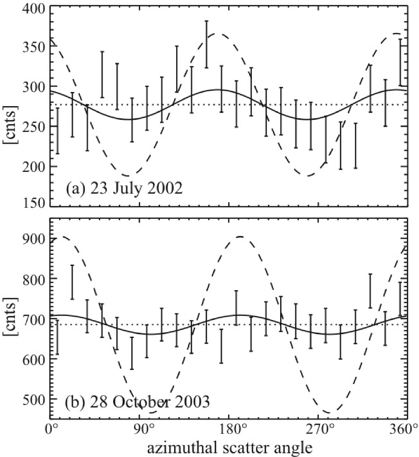
Figure 9: The 0.2-1 MeV background-subtracted ASADs for the 2002 July 23 flare (top), and the 2003 October 28 flare (bottom). Shown for comparison are the best-fit modulation (solid line), and the expected modulation for both unpolarized photons (dotted line) and 100% polarized photons (dashed line).

At this point we have three ASADs for each flare: the raw flare ASAD, the chance-coincidence ASAD, and the average-background ASAD. We subtracted the chance-coincidence ASAD and the average of the two background ASADs (scaled by the scatter livetimes) from the raw flare ASAD. This produces the residual flare ASADs for the flare photons alone, which are shown in Fig. 9.

For the two residual background-subtracted flare ASADs, we can now search for significant modulations corresponding to 180^∘ periods. For each distribution, we fit a function of the form of Eqn. 2 to determine the amplitude of the potential modulated component. Correcting for the modulation factor we can determine the intrinsic polarization fraction for the $\gamma$-ray photons from these two solar flares. In addition, we compare the modulation fit to unpolarized distributions to determine the significance of the measured signals.

4.7.1 23 July 2002

Fig. 9a shows the best-fit modulation curve to the 23 July 2002 flare scatter angle distribution. For this choice of binning, the amplitude of the modulation component is 19$\pm$8, with a 2.4$\sigma$ significance. The average is 277$\pm$10, with the uncertainty dominated by the systematic uncertainty in the background level during the flare. The ratio of these two yields the polarization of the incident flare $\gamma$-rays multiplied by the instrumental modulation factor. For this flare, $\mu_{m}\Pi_{s}$ = 0.069$\pm$0.029, the uncertainty of which includes the fact that the polarization direction is not known a priori. In order to determine the significance of this modulation, we performed a simple Monte Carlo simulation assuming an unpolarized (flat) distribution, and the average measured uncertainty, to determine how often we would randomly fit a modulation of this amplitude for an unpolarized source. Given our measurement uncertainties, the chance probability of fitting a modulation of this amplitude is 7.7%.

The minimum in the modulation curve corresponds to a direction of the polarization vector of $\eta$ = 78^∘ $\pm$ 13^∘ (north of east). Projected onto the solar disk (Fig. 10), this polarization vector is perpendicular (within its uncertainty) to the direction from the disk center toward the solar flare, which corresponds to a positive polarization by convention.

Correcting for the modulation factor, the fractional linear polarization for this flare is $\Pi_{s}$ = 0.21 $\pm$ 0.09 in the 0.2–1 MeV band. (The average measured photon energy over this band is 0.45 MeV.) For comparison, in Fig. 9a we have plotted the modulation level for a 100% polarized signal. While our absolute detection is at the marginal 2.4$\sigma$ level, we are still strongly constraining the polarization level of this flare. At the 99% confidence level (3$\sigma$), we constrain this polarization to lie within the range -6% to +48%.

4.7.2 28 October 2003

Fig. 9b shows the best-fit modulation curve to the 28 October 2003 flare scatter angle distribution. The amplitude of the modulation component is 24$\pm$12, with a 2.0$\sigma$ significance. The flat background is 685$\pm$51, with the uncertainty once again dominated by the systematic uncertainty in the background level during the flare. The ratio for this flare yields $\mu_{m}\Pi_{s}$ = 0.035$\pm$0.018. For our measurement uncertainties, the chance probability of fitting a modulation of this amplitude is 14%.

The minimum in the modulation curve corresponds to a direction of the polarization vector of $\eta$ = 101^∘ $\pm$ 15^∘ (north of east). This polarization vector is parallel to the direction from the disk center toward the solar flare (Fig. 10), corresponding to a negative polarization by convention.

Correcting for the modulation factor, the fractional linear polarization for this flare is $\Pi_{s}$ = -0.11 $\pm$ 0.05 in the 0.2–1 MeV band. (The average measured photon energy over this band is 0.50 MeV.) Once again, we have also plotted in Fig. 9b the modulation amplitude for a 100% polarized signal, demonstrating that we are strongly constraining the polarization level for this flare. At the 99% confidence level (3$\sigma$), we constrain this polarization to lie within the range -26% to +4%.

4.7.3 Null Results

As a critical test of our polarization techniques and characterization of potential systematic errors, we need to verify that signals we expect to be unpolarized do not show significant modulations. These signals include both our chance coincidence backgrounds and our true scattered-photons backgrounds, neither of which we would assume a prior to be modulated.

For the background scatters in Fig. 6, we determined the best-fit modulation amplitudes to be 3 $\pm$ 2 for the 23 July 2002 flare, and 5 $\pm$ 3 for the 28 October 2003 flare. Correcting for the modulation factor, these modulations correspond to effective polarizations of 5 $\pm$ 4% and 4 $\pm$ 3% for the two flare backgrounds, respectively. These results demonstrates that our background scatters are not polarized, and that systematic modulations are restricted for real photon-scatter events in our analysis below the 5% polarization level.

For the chance coincidence events in Fig. 5, we also determined the best-fit modulation amplitudes to be 2 $\pm$ 3 for the 23 July 2002 flare, and 10 $\pm$ 5 for the 28 October 2003 flare. (Note the fits to the 180^∘ modulations are not significantly affected by the orthogonal 360^∘ components.) Once again correcting for the modulation factor, the effective polarizations corresponding to these modulations for the chance coincidences alone are 4 $\pm$ 6% and 12 $\pm$ 6% for the two flare periods, respectively. However, when we compare the absolute value of these best-fit modulations with those measured for the background-subtracted flare ASADs above, we can see that the potential effects of these chance-coincidence modulations on the overall measured flare photon polarizations are 2 $\pm$ 3% and 4 $\pm$ 2% for the two flares respectively. Therefore, we can also limit the effects of systematically-induced modulations from the chance-coincidence events to below the 5% polarization level.

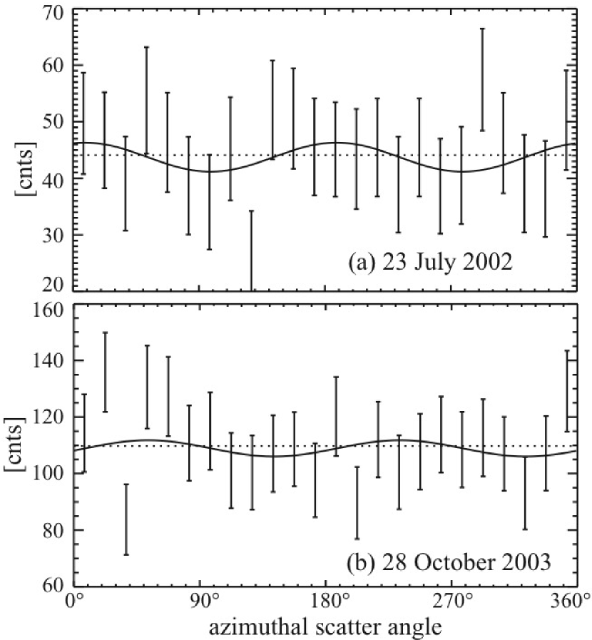
Figure 11: The 0.2-1 MeV background-subtracted ASADs for the two flares, using only backscatter events (Sec. 4.7.3). Shown for comparison are the best-fit modulation (solid line), and the average (dotted line). Since backscatter events are less sensitive to polarization than events chosen in Step 8, modulations on these ASADs should not be significant.

As a further check of null results, we repeated the polarization analysis for large-angle backscatter events in the instrument (Fig. 11). For the analysis above (ultimately deriving Fig. 9) we only accepted scatter events which were consistent with Compton scatter angles in the range 45^∘–135^∘ (Step 8 of our analysis method). This range of Compton scatter angles is the most sensitive to polarization modulations, hence this cut helped maximize the signal-to-noise. Small-angle scatters (0^∘–45^∘) and large-angle backscatters (135^∘–180^∘) are less sensitive to the incoming photon polarization, and therefore with our marginal sensitivities we expect null results for modulation curves in these cases. For our data cuts, small-angle scatters are dominated by chance coincidence events (due to favorable low-energy coincidences), while for backscatter events the chance coincidences are nearly negigible. Since we have already limited the systematic polarizations for chance coincidences, we repeated the full analysis for backscatter events to verify null results. For Steps 8 & 9, we modified the Compton kinematic cut criteria so that if either of the potential interaction orderings were consistent with a Compton scatter angle in the range 135^∘–180^∘, then the event was accepted for further analysis. The measured modulations for these backscatter events, shown in Fig. 11, are $\mu_{m}\Pi_{s}$ = 0.06$\pm$0.06 for the 2002 July 23 flare, and $\mu_{m}\Pi_{s}$ = 0.03$\pm$0.04 for the 28 October 2003 flare, consistent with our null hypothesis.

Based on these results, we are confident that we have limited the systematic uncertainties in these measurement techniques to below the 5% polarization level.

4.7.4 Energy Bands

We have presented our polarization analysis and results for the entire 0.2-1 MeV band. For completeness we have also performed the identical analysis over the 0.2-0.4 MeV band and the 0.4-1 MeV band for comparison. (Including calculation of the modulation factors for each of these smaller energy bands.) The final results of these analyses are presented in Table 2.

At first glance, the results presented in Table 2 suggest that the 2002 July 23 flare is more strongly polarized in the 0.2-0.4 MeV band than the 0.4-1 MeV band, while the 2003 October 2002 flare is more strongly polarized in the higher energy band. We stress that with our limited statistics these trends should be considered with caution.

5 Discussion

Despite the marginal detection of polarization for both of these flares, together they exhibit a few interesting properties.

Both of the flares show physically significant directions for their polarization vectors (Fig. 10), either perpendicular or parallel to the flare–disk center direction. While these detections are both marginally significant, the alignment of the polarization vectors along the two physically-possible directions supports the presumption that these are not spurious detections. It is especially intriguing that the polarization vector appears to have rotated by 90^∘ from the central disk toward the limb. If confirmed by further events, this trend will place strong constraints on the underlying beamed electrons.

Our measurements are consistent with the general expectation that the level of polarization will increase with increasing viewing angle, regardless of the underlying beamed electron distribution. For flares near the disk center (small viewing angles), the symmetry of the geometry alone should require the polarization level to approach 0%.

The levels of polarization measured are generally consistent with theoretical predictions for beamed electron distributions ($\leq$25%), and marginally inconsistent with predictions for isotropic distributions ($<$10%). In Fig. 12 we have plotted our measured polarizations along with one theoretical prediction for several $\gamma$-ray photon energies for a beamed electron model assuming a half opening angle of 30^∘ and and accelerated electron spectrum of $E^{-3.5}$ (Bai & Ramaty, 1978). Our results are generally consistent with this model, but we would clearly like to perform this analysis with several energy bands and many more flares – which is currently beyond the serendipitous RHESSI sensitivity to $\gamma$-ray polarization which we are exploiting.

We plan to continue analyses of these and other RHESSI solar flares in hopes of better constraining the $\gamma$-ray polarization as a function of both viewing angle and photon energy. These studies can clearly play an important role in illuminating the underlying electron beaming, and particle acceleration mechanisms, in solar flares. This paper has attempted to achieve two milestones in this endeavor: to verify the sensitivity of RHESSI to solar $\gamma$-ray polarization, and to establish the overall level of $\gamma$-ray polarization we can expect to observe for solar observations.

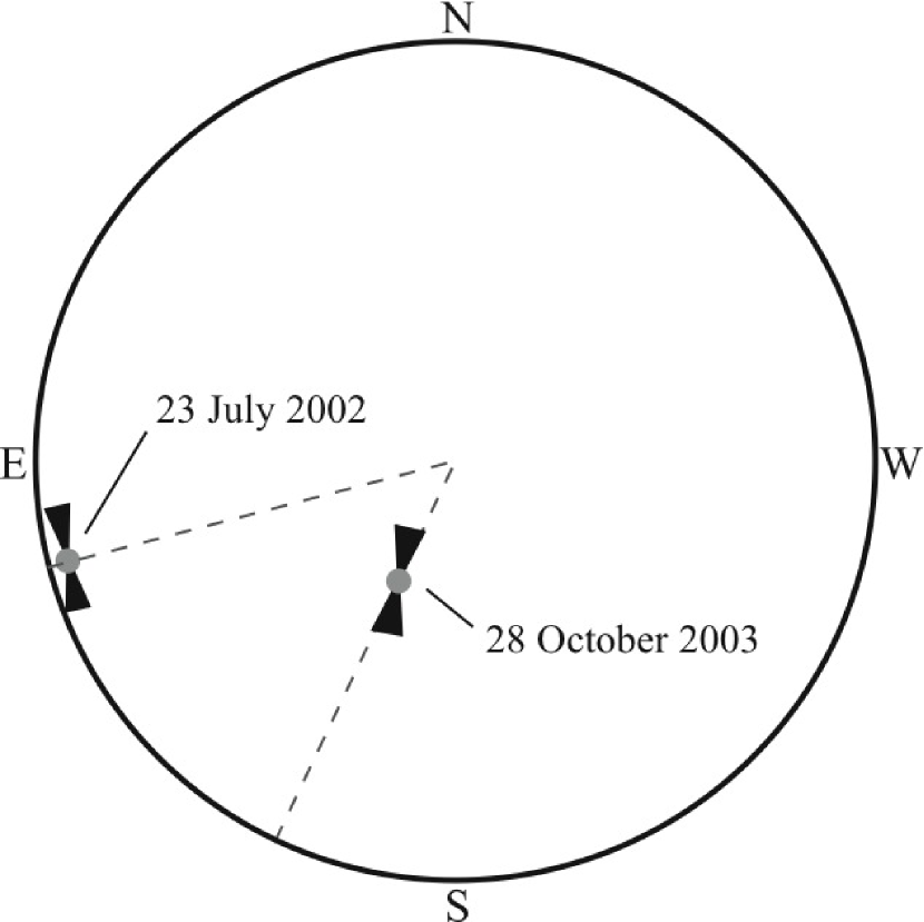
Figure 10: Diagram of the solar disk, showing the location of the two flares studied in this paper (grey circles). The $\pm 1\sigma$ limits on the 0.2-1 MeV polarization directions (black lines) are shown, as well as the radial direction from the disk center to each flare for reference.

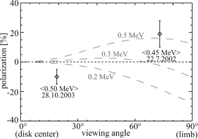
Figure 12: Our 0.2-1 MeV polarization measurements compared with a theoretical model from Bai & Ramaty (1978) for an accelerated electron spectrum of E^-3.5, beamed with into a 30^∘ half opening angle. The predictions are shown for three different photon energies: 0.2, 0.3, 0.5 MeV (dashed lines). The average photon energy for each measurement is shown for comparison. Negative polarizations correspond to polarization vectors aligned toward the center of the solar disk, while positive polarizations are perpendicular to this direction.

Table 1: Observation time intervals.

Flare	Observation	Date	Start	End
2002 July 23	Flare	2002.07.23	00:27:20 UT	00:32:20 UT
	Background 1	2002.07.22	23:00:20 UT	23:05:20 UT
	Background 2	2002.07.23	02:10:20 UT	02:15:20 UT
2003 October 28	Flare	2003.10.28	11:10:22 UT	11:18:22 UT
	Background 1	2003.10.28	09:42:22 UT	09:50:22 UT
	Background 2	2003.10.28	11:37:22 UT	11:45:22 UT

Table 2: Measured polarization amplitudes and directions.

Flare	Energy Range [MeV]	$\Pi_{s}$	$\eta$
2002 July 23	0.2–1	0.21 $\pm$ 0.09	78∘ $\pm$ 13∘
	0.2–0.4	0.26 $\pm$ 0.12	65∘ $\pm$ 13∘
	0.4–1	0.17 $\pm$ 0.15	–
2003 October 28	0.2–1	-0.11 $\pm$ 0.05	101∘ $\pm$ 15∘
	0.2–0.4	0.07 $\pm$ 0.07	–
	0.4–1	-0.25 $\pm$ 0.09	113∘ $\pm$ 10∘

References

- Bai & Ramaty (1978) Bai, T., & Ramaty, R., 1978, ApJ, 219, 705
- Brown (1972) Brown, J. C., 1972, Sol. Phys., 26, 441
- Chanan, Emslie, & Novick (1988) Chanan, G., Emslie, A. G., & Novick, R., 1988, Sol. Phys., 118, 309
- Charikov, Guzman, & Kudryavstev (1996) Charikov, Ju. E., Guzman, A. B., & Kudryavtsev, I. V., 1996, A&A, 308, 924
- Coburn & Boggs (2003) Coburn, W., & Boggs, S. E., 2003, Nature, 423, 415
- Elwert (1968) Elwart, G., 1968, in K. O. Kiepenheuer (ed.), ’Structure and Development of Solar Active Regions’, IAU Symp., 35, 44
- Haug (1972) Haug, E., 1972, Sol. Phys., 25, 425
- Hurford et al. (2002) Hurford, G. J., et al., 2002, Sol. Phys., 210, 61
- Korchak (1967) Korchak, A. A., 1967, Soviet Phys. Dokl., 12, 192
- Langer & Petrosian (1977) Langer, S. H., & Petrosian, V., 1977, ApJ, 215, 666
- Leach & Petrosian (1983) Leach, J., & Petrosian, V., 1983, ApJ, 269, 715
- Leach, Emslie, & Petrosian (1985) Leach, J., Emslie, A. G, & Petrosian, V., 1985, Sol. Phys., 96, 1985
- Lei, Dean & Hills (1997) Lei, F., Dean, A. J., & Hills, A. G., 1997, Space Sci. Rev., 82, 309
- Lin et al. (2002) Lin, R. P., et al., 2002, Sol. Phys., 210, 33
- Lin et al. (2003) Lin, R. P., et al., 2003, ApJ, 595, L69
- McConnell et al. (2002) McConnell, M. L., et al., 2002, Sol. Phys., 210, 125
- McConnell et al. (2004) McConnell, M. L., et al., 2004, Adv. Space Res., 34, 462
- Nakada et al. (1974) Nakada, M. P., et al., 1974, Sol. Phys., 37, 429
- Novick (1975) Novick, R., 1975, Space Sci. Rev., 18, 389
- Smith et al. (2002) Smith, D. M., et al., 2002, Sol. Phys., 210, 33
- Smith et al. (2003) Smith, D. M., et al., 2003, ApJ, 595, L81
- Sturner et al. (2000) Sturner, S., et al., 2000, in M. L. McConnell & J. M. Ryan (eds.), ’Proceedings of the 5th Compton Symposium’, AIP Conf. Proc., 510, 814
- Tindo et al. (1970) Tindo, I. P., et al., 1970, Sol. Phys., 14, 204
- Tindo et al. (1976) Tindo, I. P., et al., 1976, Sol. Phys., 46, 219
- Tramiel, Chanan, & Novick (1984) Tramiel, L. J., Chanan, G. A., & Novick, R., 1984, ApJ, 280, 440
- Wigger et al. (2004) Wigger, C., et al., 2004, ApJ, 613, 1008
- Wunderer et al. (2004) Wunderer, C. B., et al., 2004, Proc. 5th INTEGRAL Workshop, ESA SP-552, 913
- Zehnder et al. (2003) Zehnder, A., et al., 2003, Proc. SPIE, 4853, 41
- Zharakova, Brown, & Syniavskii (1995) Zharkova, V. V., Brown, J. C., & Syniavskii, D. V., 1995, A&A, 304, 284