A compact flare eclipsed in the corona of SV Cam

The eclipsing active binary SV Cam (G0V/K6V, $P_{\rm orb}$=0.593071 d) was observed with XMM-Newton during two campaigns in 2001 and 2003. No eclipses in the quiescent emission are clearly identified, but a flare was eclipsed during the 2001 campaign, allowing us to strongly constrain, from purely geometrical considerations, the position and size of the event: the flare is compact and it is formed at a latitude below 65$\degr$. The size, temperature and Emission Measure of the flare imply an electron density of $\log n_{\rm e}$ (cm^-3)$\sim$10.6–13.3 and a magnetic field of $\sim$65–1400 G in order to confine the plasma, consistent with the measurements that are obtained from density-sensitive line ratios in other similar active stars. Average emission seems to come from either extended or polar regions because of lack of eclipses. The Emission Measure Distribution, coronal abundances and characteristics of variability are very similar to other active stars such as AB Dor (K1V).

1 Introduction

The analysis of stellar coronae is commonly based on several aspects such as thermal structure, coronal abundances, stellar flares and analysis of eclipses. Since the first high resolution spectra in X-rays and XUV it has become evident that low activity stars, such as the Sun, have a thermal structure substantially different from that of active stars. Active stars, such as AB Dor or Capella are dominated by material at $T\sim 10$ MK, much hotter than the solar corona ($T\sim 2$ MK), and display a substantially larger number of flares (Dupree et al., 1993; Schrijver et al., 1995; Bowyer et al., 2000; Sanz-Forcada et al., 2003a; Huenemoerder et al., 2001; Maggio et al., 2004; Favata & Micela, 2003, and references therein). The thermal structure found in active stars is normally interpreted as the combination of different families of coronal loops (e.g. Griffiths & Jordan, 1998; Jardine et al., 2002), and it is reminiscent of the thermal structure found in some solar flares. The analysis of eclipses and rotational modulation raised the question on whether these loops with peak temperature around $\log T$(K)$\sim$6.9 are linked to a given coronal region such as the stellar poles (Brickhouse & Dupree, 1998; Schmitt & Favata, 1999), where photospheric spots are usually detected. One of the ways to get further insight in the knowledge of the coronae of active stars is to observe eclipsing binaries containing active stars, that may allow us to estimate the size and geometrical position of the emitting regions and to derive other characteristics. Coronal abundances of active stars also tend to show a rather low abundance of low-FIP elements when they are compared to the solar photosphere, although comparison with their own photospheric values may result in a composition consistent with that of the photosphere of the star (Sanz-Forcada et al., 2004), this still being an open debate.

The eclipsing binary SV Cam (HD 44982) is a well-studied spectroscopic RS CVn system at a distance of 85 pc (Perryman et al., 1997), formed by a spectroscopic binary (G0V/K6V, Lehmann et al., 2002) and the likely presence of a third (less massive) body in a wide orbit (Albayrak et al., 2001). SV Cam has a short orbital period ($P_{\rm orb}$=0.593071 d, Pojmanski, 1998), with locked rotation that causes enhanced stellar activity in the system. SV Cam has been detected by ROSAT (Hempelmann et al., 1997), but the low statistics of the observation did not allow us to clearly identify the presence of eclipses in the X-ray band. Optical observations reveal the presence of spots in the primary star, but the low luminosity of the secondary ($\sim$15% of the total) does not allow us to identify such features on the cooler object (Hempelmann et al., 1997; Kjurkchieva et al., 2002; Zboril & Djurašević, 2003, and references therein). The H$\alpha$ and Ca IR triplet profiles are filled in due to chromospheric activity in the secondary star (Montes et al., 1995; Pojmanski, 1998; Kjurkchieva et al., 2002). Recently, Jeffers (2005) found large polar spots in the photosphere of the primary star using Doppler imaging techniques, as well as the presence of smaller spots on the rest of the stellar surface (as is typical of active stars).

The outline of this paper is as follows: Sect. 2 describes the observations along with a brief description of the analysis techniques; the results are explained in Sect. 3, followed by a discussion, and Sect. 4 presents the conclusions.

Figure 1: SV Cam light curves (MOS1+MOS2 and PN respectively) in the 2003 campaign, with 1-$\sigma$ error bars. The upper axis reports the orbital phase, with $T_{0}$=HJD 2449350.3037 corresponding to primary (G0V) star located behind the secondary (K6V) star, and $P_{\rm orb}$=0.593071 d (Pojmanski, 1998). Solid lines mark the times when photospheric eclipses take place.

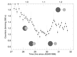
Figure 2: Upper panel: Same as Fig. 1, but for the 2001 campaign (only MOS data are available). An eclipse in the flare, around $\phi\sim$1.1, is displayed in the lower panel with a bin size of 300 s. Dotted lines indicate the phases used for the four contacts. The relative positions of the stars during the contacts are also indicated.

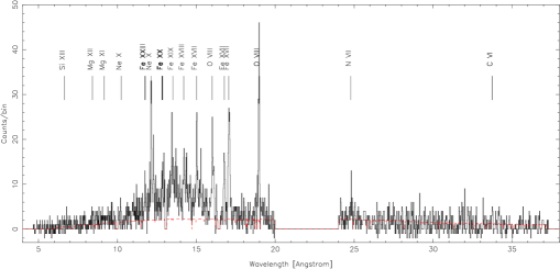
Figure 3: RGS 2 spectrum of SV Cam in October 2003. The dashed line represents the continuum predicted by the derived EMD. A false continuum is created by the extended instrumental line profiles.

2 Observations

SV Cam was observed with XMM-Newton (P.I. F. Favata) in March 2001 (rev. #238) for 65 ks, but due to technical problems and high background part of the data were not usable, in particular the PN data. The target was observed again in October 2003 (rev. #700) for 67 ks. XMM-Newton carries out simultaneous observation with the EPIC (European Imaging Photon Camera) PN and MOS detectors (sensitivity range 0.15–15 keV and 0.2–10 keV respectively), and with the RGS (Reflection Grating Spectrometer, den Herder et al., 2001) ($\lambda\lambda\sim$6–38 Å, $\lambda$/$\Delta\lambda\sim$100–500). The data have been reduced employing the standard SAS (Science Analysis Software) version 6.1.0 package, removing in the RGS spectra the time intervals when the background was higher than 0.7 cts/s in CCD #9, to ensure a “clean” spectrum. Light curves were obtained by selecting a circle centered on the source in the EPIC-PN and EPIC-MOS images, and subtracting the background count rate taken from a nearby area (Figs. 1, 2). In the 2001 campaign the EPIC data were split in three intervals due to high flaring background. In the PN, the third interval suffered from technical problems and therefore we display only the combined MOS1+MOS2 light curve (data from both detectors were obtained separately and then combined in the light curve after fixing the time shift present between MOS 1 and 2). Mid-resolution spectra were obtained with EPIC detectors in the range 0.3–10 keV, once the intervals with high background level were excluded. The average X-ray luminosity ($L_{\rm X}$) was calculated from the PN spectra of the two campaigns (the whole interval was used for 2003, and only the first interval for 2001), resulting in values of $L_{\rm X}=1.7\times 10^{30}$ and $L_{\rm X}=2.4\times 10^{30}$ erg s^-1 in the range 6–20 Å (0.62–2.1 keV) for 2001 and 2003 respectively, and $L_{\rm X}=2.6\times 10^{30}$ erg s^-1 and $L_{\rm X}=3.9\times 10^{30}$ erg s^-1 in the range 5–100 Å (0.12–2.4 keV), the range covered by ROSAT/PSPC. This indicates an increase in the X-ray flux by $\ga$50 % between the two observations, with $L_{\rm X}/L_{\rm bol}=5.6\times 10^{-4}$ and $L_{\rm X}/L_{\rm bol}=8.5\times 10^{-4}$ calculated over the 5–100 Å range.

The rich RGS spectrum taken in 2003 (Fig. 3) has been used to calculate the thermal structure (the Emission Measure Distribution, EMD) and coronal abundances of SV Cam, following the method described in Sanz-Forcada et al. (2003b): line fluxes are measured in the RGS spectrum, and a trial EMD and a set of coronal abundances are combined with an atomic plasma model in order to compare observed and predicted line fluxes. The EMD and abundances are then corrected to get the best approximation between the two sets of line fluxes values, and an iterative process is carried out in order to better determine the continuum position that is employed to measure the line fluxes in RGS. The determination of abundances during the process is made as follows: only Fe lines are used initially to determine the EMD; then the abundance of Ne is fixed in the temperature domain where the EMD is known, and the EMD is extended afterwards to the rest of the temperature domain covered by Ne; the rest of elements are added sequentially following the same process. This assumes that the relative elemental abundances are constant throughout the corona. Such an approach has shown good consistency between results of the different detectors capable of achieving high-spectral resolution of stellar coronae (Sanz-Forcada et al., 2003b). In this analysis we have measured the line fluxes (Table 4) using the Interactive Spectral Interpretation System (ISIS, Houck & Denicola, 2000) software package, through convolution of the spectral response. The measured line fluxes were then corrected for interstellar medium absorption (ISM) using a value of $\log\leavevmode\nobreak\ N_{\rm H}({\rm cm}^{-2})\sim 19.7$ (although such a correction has very little influence on the result). The EMD was reconstructed using a step in temperature of 0.1 dex, the same employed in the Astrophysical Plasma Emission Database (APED v1.3.1, Smith et al., 2001), the plasma atomic model used in our analysis.

3 Results and discussion

3.1 Light curves

The light curves of SV Cam reveal a high level of variability in the corona of this system, with flares clearly identified in both campaigns (Figs. 1, 2). In 2001 a drop in counts occurred while a flare was decaying, reaching the quiescent levels at phase $\phi\sim 1.1$, and then returning to the flaring levels. We interpret this decay as an eclipse of the flaring region, with the totality of this region being occulted. The light curve of the hardness ratio, defined as HR=Hard/Soft where Hard and Soft are the fluxes in the bands 1–10 keV and 0.3–1 keV respectively (Fig. 4) is sensitive to the changes in temperature. The flare is well identified by the rise in temperature, with a subsequent decay. During the eclipse, at $\phi\sim 1.1$ the temperature drops to the level previous to the flare. The existence of two flares could also explain this behaviour, but two further arguments strengthen the hypothesis of an eclipse taking place: (i) the decay of the first peak changes suddenly to a much steeper one (at $\phi\sim$1.02); although some cases with two decays have been reported in the literature, the second decay is always less steep than the first, while in the case of SV Cam we observe a steeper decay, something not observed to date; (ii) the light curve shows a strong symmetry between the points that we interpret as responsible for the 4 contacts, a symmetry much more likely in an eclipsing phenomenon. Therefore, although we cannot completely rule out a sequence of two flares, we consider the hypothesis of an eclipse as the most likely. We can use this eclipse to derive some information of the flare, as we will explain in detail below.

In the 2003 campaign (Fig. 1) the observation appears to take place during the decay of a flare, with a new flare developing at $\phi\sim 1.6$. We find no evidence of an eclipse in the light curve. Therefore, from the two campaigns we can conclude that most of the coronal emission is not being occulted during eclipses, and therefore the non-flaring emission is either very extended or it originates at high latitudes on the primary.

Figure 4: Hardness ratio (HR), defined as HR=Hard/Soft, where Hard and Soft are the fluxes in the bands 1–10 keV and 0.3–1 keV respectively. Note the drop in the HR during the eclipse, at $\phi\sim 1.1$.

Regarding the variability of the source, we have made an analysis of the amplitude variability, defining amplitude as $W=L_{\rm X}$/$L_{\rm min}$, where $L_{\rm min}$ is the assumed quiescent value of the light curves (corresponding to the mode of the count rate distribution), following Sanz-Forcada & Micela (2002). The amplitude variability curve, shown in Fig. 5 tells us how activity “behaves” in a star or group of stars. In Fig. 5 we compare the case of the two observations of SV Cam (each with its own $L_{\rm min}$) with the K1V active star AB Dor (Sanz-Forcada et al., in preparation) and a group of M stars (Marino et al., 2000). The observations of AB Dor were made with same instrument (EPIC MOS 1+MOS 2), during XMM-Newton revolutions #162, 205, 266, 338, 429 and 462. The M stars were observed with ROSAT in the range $\Delta E$=0.12–2 keV. Although the spectral range and time scale of the observations is different, a contrast between the variability in active M stars and that from the active G and K dwarfs SV Cam and AB Dor is quite evident. Results from EUVE ($\Delta E$=0.07–0.15 keV) for the dM star AD Leo have shown very similar results to those of ROSAT (Sanz-Forcada & Micela, 2002). Among the two observations of SV Cam, in 2003 there is a higher level of emission, but a lower level of variability than in 2001. The latter is also remarkably similar to the average behavior of AB Dor.

The whole view of the variability in SV Cam shows an active star with a quiescent level rather difficult to identify, and with flaring activity going on in the two campaigns. No eclipses out of flares could be identified, but an eclipse during a flare has been observed, and it will be the subject of further analysis below. These light curves indicate that the “quiescent” coronal emission comes either from an extended region, or from high latitudes of the primary star.

3.2 An eclipsed flare in SV Cam

To determine the geometry of the occulted flare, we have considered the four contacts of the eclipse, identified at phases 1.024, 1.065, 1.118, 1.159 (Fig. 2) in the light curve with 300 s binning. To simplify the problem, we assume that the emitting region has a spherical shape, and we characterize the flare with four variables: latitude ($\theta$), longitude ($\lambda$, with origin 0 the meridian of the each star that is in front of the observer at $\phi$=0), height over the center of the hosting star ($h$) and the size of the spherical emitting region ($R_{3}$). We have made a grid of values for the 4 variables, and we then calculated the times when the four contacts of the eclipse take place for each set of values. We considered as valid results those that agree within 300 s (1 bin) with the measured times. There are four possible scenarios for the eclipse to happen:

1. primary star hosting the flare which is eclipsed by the secondary,

2. self-eclipse in the secondary star,

3. self-eclipse in the primary star,

4. self-eclipse by the primary star actually starting (first contact) when the second star hides the flare, and ending behind the primary.

Figure 5: Normalized cumulative distribution of the amplitude ($W=L_{\rm X}/L_{\rm min}$) variability in SV Cam in the two observing campaigns, as measured in EPIC MOS1+MOS2 count rates. Also displayed are the ROSAT/PSPC ($\Delta E$=0.12–2 keV) observations of a sample of M stars (Marino et al., 2000) and the MOS 1+MOS 2 amplitude variability in observations of AB Dor (see text).

.

Possible solutions are plotted in Fig. 6 and listed in Table 1, and we will refer to them as cases 1, 2, 3 and 4 according to this Table.

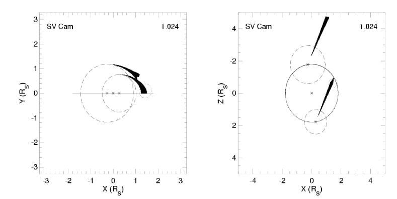
Figure 6: Relative positions of the two stars (dashed lines) during first contact ($\phi$=1.0240), as seen from the front (left panel) and top (right panel). The solid line marks the orbit of the stars around the center of mass, while three asterisks mark the central positions of the two stars at first contact, and the center of the orbit. All the possible results are represented with black points indicating the center of the emitting region (only the solutions in the northern hemisphere are represented). An example of the eclipsed region with a size of $R_{3}$=0.28 $R_{\odot}$ is shown in dotted line.

We make use of the orbital data calculated by Lehmann et al. (2002): $R_{1}$, $R_{2}$=1.18, 0.76 R_⊙, $a_{12}$=3.60 R_⊙ (axis of the orbit), $i$=89.6$\degr$ (we can safely assume $i$=90 to simplify equations), $M_{1}$, $M_{2}$=1.09, 0.70 M_⊙ and circular orbits. The solutions found in the first two cases (flare hosted by primary or secondary, but eclipsed by the secondary) correspond actually to the same points in the 3-D space. The equations corresponding to the first case (primary star hosting a flare eclipsed by secondary) are:

$$x_{1}=-\frac{1}{2}\;a\sin(\phi),\quad y_{1}=0,\quad z_{1}=-\frac{1}{2}\;a\cos{\phi}$$

$$x_{2}=-x_{1},\quad y_{2}=0,\quad z_{2}=-z_{1}$$

$$x_{3}=x_{1}+h\cos(\theta)\sin(\phi+\lambda),\quad y_{3}=y_{1}+h\sin(\theta),\quad$$

$$z_{3}=z_{1}+h\cos(\theta)\cos(\phi+\lambda)$$

where $x$, $y$ correspond to the plane in front of the observer (Fig. 6), and $z$ is perpendicular to this plane (positive towards the observer). $x_{3}$, $y_{3}$, $z_{3}$ correspond to the position of the emitting region of the flare. In the first and fourth contacts the distance between the center of the flare and the center of secondary star must be:

$$\Delta_{1}=\sqrt{(R_{2}+R_{3})^{2}-(y_{3}-y_{2})^{2}}$$

and similarly, in the second and third contacts:

$$\Delta_{2}=\sqrt{(R_{2}-R_{3})^{2}-(y_{3}-y_{2})^{2}}$$

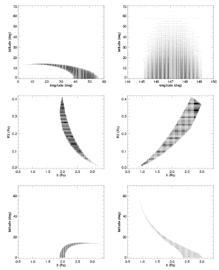
Figure 9: Left: Results in case 1 (primary flaring, secondary eclipsing). Right: Results in case 2 (self-eclipse in secondary).

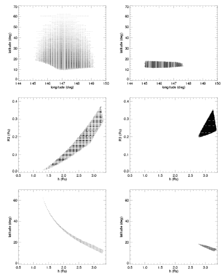
Figure 10: Left: Results in case 3 (self-eclipse entirely in primary). Right: Results in case 4 (primary flaring, eclipse starts in secondary, ends in primary).

Thus, in the four positions we will have four equations: $x_{3}=x_{2}+\Delta_{1},\quad x_{3}=x_{2}+\Delta_{2}\quad x_{3}=x_{2}-\Delta_{2}\quad x_{3}=x_{2}-\Delta_{1}$ respectively, that we can use to calculate numerically the times of the four contacts for each point of the grid. Some geometrical constraints can be added to ensure the totality of the eclipse ($y_{3}+R_{3}\leq y_{2}+R_{2}$) and a valid position in $z$ ($z_{3}+\sqrt{(R_{2}+R_{3})^{2}-(y_{3}-y_{2})^{2}}<z_{2}$). Similar equations can be easily derived for the other cases. An additional constraint was imposed in the cases 3 and 4, the only scenarios in which $h$ reaches values larger than $a$: the centrifugal force must be lower than the resulting gravitational forces of the two stars. In this way, $h$+$R_{3}$ must be lower than $\sim$3.6 R_⊙. The results found are shown in Table 1 and in Figs. 9 and 10. The trends relating the different variables are: in case 1, for an increasing $h$, $R_{3}$ and $\lambda$ decrease, and $\theta$ increases; for the other 3 cases an increase in $h$ yields an increase in $R_{3}$ and a decrease in $\theta$, with no trend for $\lambda$.

Table 1: Range of possible solutions (northern hemisphere only) of the eclipse of a flare in 2003.

Flaring star	Ecl. star	$\theta$($\degr$)	$\lambda$($\degr$)	$h$ (R⊙)	$R_{3}$ (R⊙)	$\log n_{\rm e}$ (cm-3)	$B$ (G)
Pri	Sec	0–14	4.7–55.7	1.91–3.28	0.012–0.41	10.6–12.9	66–930
Sec	Sec	0–65	145.1–149.1	0.83–2.99	0.006–0.41	10.6–13.4	66–1600
Pri	Pri	9.7–62	145.1–149.1	1.31–3.30	0.013–0.37	10.7–12.8	72–880
Pri	S+P	12–18	145.0–147.6	2.77–3.36	0.20–0.36	10.7–11.1	74–110
All results		0–65	$\sim$5–56 or $\sim$146	0.83–3.36	0.006–0.41	10.6–13.4	66–1600

We can also estimate the electron density ($n_{\rm e}$) of the emitting region by calculating the Emission Measure (EM) before ($\phi\la$0.6) and during the flare prior to the eclipse ($\phi\sim 0.87-1.02$) through a fit of the MOS spectra. A fit using 3 temperatures resulted in an average value of $\log T$ (K)=7.17 and $\log$ EM (cm^-3)=53.17 in quiescence and $\log T$ (K)=7.22 and $\log$ EM (cm^-3)=53.38 during the flare. Since we can define EM$\sim 0.8\,n_{\rm e}^{2}\,V$, it is possible to get the density $n_{\rm e}$ from the net flare EM, using $V=4\pi/3R_{3}^{3}$ (see Table 1). If we consider that the magnetic pressure, $B^{2}/(8\pi)$, should be at least as large as the electron pressure ($2n_{e}kT$), we can get the minimum magnetic field necessary to have a stable structure in the flare.

The analysis of the eclipse leads to several interesting conclusions: (i) the flare takes place at regions with $\theta\la 65\degr$; (ii) the emitting region is compact in size ($R_{3}\la 0.41$ R_⊙), implying values of the electron density consistent with those calculated from the Chandra and XMM-Newton spectra of active stars at different temperatures (Sanz-Forcada et al., 2003b; Ness et al., 2004; Testa et al., 2004); (iii) the emitting region is not necessarily attached to the surface of the star (the minimum $h$ found – in case 2 – implies also the minimum size and the highest values of density) and therefore the loop of the flare likely has its emission concentrated in the apex.

3.3 Eclipses and flares

There are a few cases in the literature where the flares have been eclipsed. Such an event is very useful to constrain some of the characteristics of the flaring region. The technique most commonly used derives the position of the flare from the whole eclipse light curve. This was the case of two flares in the secondary star of Algol (B8V/K2III): Schmitt & Favata (1999) using BeppoSAX, observed a flare in a polar region (there was no rotational modulation), with a loop height/size $\la$0.6 R_∗ (2 R_⊙), resulting in densities of at least $\sim$10¹¹ cm^-3 and $B\ga 500$ G; Schmitt et al. (2003) using a more detailed analysis, studied another flare in Algol observed with XMM-Newton, resulting in a nearly equatorial location with loop heights $\sim$0.1 R_∗ (0.3 R_⊙) and densities of several times 10¹¹ cm^-3, resulting again in $B\sim 400$ G as the minimum to accommodate the electron pressure found. More recently, Mitra-Kraev et al. (2005) used the oscillations observed in a flare of the dM star AT Mic to constrain the flare loop length to $\sim$0.36 R_⊙ and $B\sim 100$ G. The first case reported in the literature was an analysis of an ASCA light curve with lower statistics of VW Cep (Choi & Dotani, 1998). The authors use rather qualitative assessments, and the ingress and egress times of the eclipse, to conclude that the flare should be occuring near the pole, at a height/size of 0.5 R_∗ ($\sim$0.5 R_⊙) and $B\sim 80$ G.

Figure 7: Emission Measure Distribution of SV Cam in Oct. 2003. Thin lines represent the relative contribution function for each ion (the emissivity function weighted by the EMD at each point). Small numbers indicate the ionization stages of the species. The observed to predicted line flux ratios for the ion stages in the upper figure are plotted in the lower figure. Dotted lines denote a factor of 2.

Although the techniques employed do not result in an exact determination of the geometry of the loop, all these studies need for a large (at least 100 G) magnetic field in order to explain the presence of loops that have a relatively compact sizes. We will apply the technique used for SV Cam to the analysis of these flares in a future publication (Sanz-Forcada et al., in preparation).

3.4 Thermal structure and abundances

The analysis of the thermal structure reveals an EMD (Fig. 7, Table 2) very similar to the other active stars (Sanz-Forcada et al., 2003a), in which the EMD is dominated by a peak of material at $\log T$(K)$\sim$6.9 with strong dependency on the rotational period of the star, and with a large amount of material at higher temperatures in the case of SV Cam that is also supported by the detection in the EPIC-PN spectrum of the Fe xxv complex at 6.7 keV. In this case the lack of statistics prevents the measurement of the O vii He-like triplet that would be useful to determine the electron density at $\log T$(K)$\sim$6.3.

Coronal abundances (Table 3, Fig. 8) are not as metal-deficient relative to the Sun as they are for other active stars (Huenemoerder et al., 2001; Audard et al., 2003; Sanz-Forcada et al., 2003b, 2004), although a [Ne/Fe]=0.40$\pm$0.13 is lower than for other stars of its activity level (e.g., Drake et al., 2001). If we consider the uncertainties, most values are consistent with solar photosperic abundances. Most of the uncertainty comes from the determination of the Fe abundance, given the difficulties in setting the continuum in the RGS spectrum. The rest of the abundances were all calculated relative to Fe, therefore any shift in its value will affect the others. The lack of information on the photospheric abundances of SV Cam prevents us from drawing any conclusions on the changes in abundance pattern taking place in the corona, as it has been shown in Sanz-Forcada et al. (2004).

Table 2: Emission Measure Distribution of SV Cam in Oct. 2003.

log $T$ (K)	log $\int N_{\rm e}N_{\rm H}{\rm d}V$ (cm-3)a
6.0	51.50:
6.1	50.40:
6.2	50.80${}^{+0.20}_{-0.40}$
6.3	51.00${}^{+0.10}_{-0.30}$
6.4	50.70${}^{+0.20}_{-0.40}$
6.5	50.80${}^{+0.20}_{-0.40}$
6.6	51.10${}^{+0.20}_{-0.40}$
6.7	51.40${}^{+0.30}_{-0.30}$
6.8	51.85${}^{+0.25}_{-0.25}$
6.9	52.75${}^{+0.00}_{-0.00}$
7.0	52.50${}^{+0.20}_{-0.20}$
7.1	52.60${}^{+0.20}_{-0.20}$
7.2	52.45${}^{+0.15}_{-0.25}$
7.3	52.30${}^{+0.20}_{-0.30}$
7.4	52.00${}^{+0.30}_{-0.30}$
7.5	51.20:
7.6	49.60:

^aEmission Measure, where $N_{\rm e}$ and $N_{\rm H}$ are electron and hydrogen densities, in cm^-3. Error bars provided are not independent between the different temperatures, see text.

Figure 8: SV Cam coronal abundances in Oct. 2003. Dashed line indicates solar photospheric abundances by Anders & Grevesse (1989).

4 Conclusions

The corona of SV Cam has shown a very similar thermal pattern to all the active stars, and although coronal abundances were calculated, no conclusion can be drawn due to the lack of information on the photospheric abundances. The most interesting information on SV Cam comes from its light curves. The SV Cam corona was shown to be variable, with a change in flux of at least $\sim$ 50% in 36 months, and several flares. No coronal eclipses have been unequivocally identified during quiescence, but the eclipse of a flare allowed us to constrain the size and location of the emitting region of the flare. We found that the flare is compact ($R_{3}\sim 0.01-0.4\leavevmode\nobreak\ {\rm R}_{\odot}$), thus implying a range of electron densities that is consistent with the values calculated from line ratios at different temperatures for active stars. While the quiescent emission of the corona seems to be extended or concentrated at high latitudes, the eclipsed flare has $\theta\la 65\degr$, in contrast with the polar flare observed in Algol by Schmitt & Favata (1999).

Table 3: Coronal abundances of the elements ([X/H], solar units) in SV Cam.

X	FIP	Referencea	[X/H]
	eV	solar value	SV Cam
Ni	7.63	6.25	0.48$\pm$0.12
Mg	7.64	7.58	$-$0.09$\pm$0.20
Fe	7.87	7.67	$-$0.20$\pm$0.20
Si	8.15	7.55	$-$0.16$\pm$0.39
S	10.36	7.21	$-$0.31$\pm$0.35
C	11.26	8.56	$-$0.08$\pm$0.25
O	13.61	8.93	$-$0.02$\pm$0.13
N	14.53	8.05	$-$0.10$\pm$0.16
Ar	15.76	6.56	$-$0.40$\pm$0.45
Ne	21.56	8.09	0.20$\pm$0.13

^a Solar photospheric abundances from Anders & Grevesse (1989), adopted in this work, are expressed in logarithmic scale. Note that several values have been updated in the literature, most notably the cases of Fe (now 7.45, Asplund et al., 2000), O (now $\sim$8.7, Allende Prieto et al., 2001; Holweger, 2001) and C (now 8.39, Allende Prieto et al., 2002).

Table 4: XMM/RGS line fluxes of SV Cam^a

Ion	$\lambda$model	log $T_{\mathrm{max}}$	$F_{\mathrm{obs}}$	S/N	ratio	Blends
Si xiii	6.6479	7.0	1.84e-14	3.9	-0.27	Si xiii 6.6882
Si xiii	6.7403	7.0	3.00e-14	3.7	0.31	Mg xii 6.7378, Si xiii 6.7432
Mg xii	8.4192	7.0	3.48e-14	5.3	-0.00	Mg xii 8.4246
Mg xi	9.1687	6.8	1.42e-14	5.4	-0.16
Mg xi	9.2312	6.8	3.31e-14	8.4	0.25	Fe xxi 9.1944, Ni xix 9.2540, Fe xxii 9.2630, Mg xi 9.3143, Ni xxv 9.3400
Fe xxi	9.4797	7.0	2.23e-14	7.1	0.35	Ne x 9.4807, 9.4809
No id.	10.0200		2.03e-14	5.1	…	Na xi 10.0232, 10.0286
Ne x	10.2385	6.8	1.82e-14	7.0	-0.08	Ne x 10.2396
Fe xxiv	10.6190	7.3	2.84e-14	6.7	0.08	Fe xix 10.6414, 10.6491, 10.6840, Fe xvii 10.6570, Fe xxiv 10.6630
Fe xvii	10.7700	6.8	6.05e-15	3.1	-0.53	Ni xxiii 10.7214, 10.8491 , Fe xix 10.8160
Fe xxiii	11.0190	7.2	3.16e-14	7.3	-0.01	Fe xxiii 10.9810, Fe xxiv 11.0290
Fe xxiv	11.1760	7.3	1.47e-14	5.1	-0.07	Fe xvii 11.1310, Fe xxiv 11.1870
Fe xvii	11.2540	6.8	1.96e-14	5.9	0.12	Ni xxii 11.2118, Fe xxiv 11.2680, Fe xxiii 11.2850, Ni xxi 11.2908
Fe xviii	11.4230	6.9	2.41e-14	6.5	0.07	Fe xxii 11.4270, Fe xxiv 11.4320, Fe xxiii 11.4580
Fe xviii	11.5270	6.9	8.50e-15	3.8	-0.40	Fe xviii 11.5270, Fe xxii 11.4900, Ni xix 11.5390, Ni xxi 11.5390, Ne ix 11.5440
Fe xxii	11.7700	7.1	5.77e-14	10.5	-0.08	Fe xxiii 11.7360, Ni xx 11.8320, 11.8460
Fe xxii	11.9770	7.1	1.67e-14	5.7	0.11	Fe xxii 11.9320, Fe xxi 11.9750
Ne x	12.1320	6.8	1.24e-13	15.8	0.15	Ne x 12.1321
Fe xxi	12.2840	7.0	3.47e-14	8.4	-0.20	Fe xvii 12.2660
Ni xix	12.4350	6.9	3.23e-14	8.2	0.00
Fe xx	12.8240	7.0	4.23e-14	9.4	-0.24	Fe xxi 12.8220, Fe xx 12.8460, 12.8640
Fe xx	12.9650	7.0	3.63e-14	8.4	0.01	Fe xx 12.9120, 12.9920, 13.0240 , Fe xix 12.9330, 13.0220, Fe xxii 12.9530
Fe xx	13.1530	7.0	3.13e-14	7.7	0.00	Fe xx 13.1370, 13.2740, Fe xxii 13.2360, Fe xxi 13.2487, Ni xx 13.3090
Ne ix	13.4473	6.6	3.46e-14	8.8	-0.18	Fe xx 13.3850, Fe xix 13.4230, 13.4620
Fe xix	13.5180	6.9	5.84e-14	11.5	-0.02	Fe xix 13.4970, Fe xxi 13.5070, Ne ix 13.5531
Ne ix	13.6990	6.6	3.03e-14	8.4	0.05	Fe xix 13.6450, 13.6752, 13.7315, 13.7458
Fe xix	13.7950	6.9	4.04e-14	12.9	0.04	Fe xx 13.7670, Ni xix 13.7790, Fe xvii 13.8250
Fe xxi	14.0080	7.0	2.60e-14	7.8	-0.19	Ni xix 14.0430, 14.0770
Fe xviii	14.2080	6.9	4.72e-14	11.9	-0.17	Fe xviii 14.2560, Fe xx 14.2670
Fe xviii	14.3730	6.9	2.47e-14	6.6	-0.17	Fe xx 14.3318, 14.4207, 14.4600, Fe xviii 14.3430, 14.4250, 14.4392
Fe xviii	14.5340	6.9	1.10e-14	5.3	-0.25	Fe xviii 14.4856, 14.5056, 14.5710, 14.6011
O viii	14.8205	6.5	8.96e-15	6.6	0.06	Fe xviii 14.7820, 14.7867, O viii 14.8207, Fe xx 14.8276
Fe xvii	15.0140	6.7	8.14e-14	19.8	-0.13	Fe xix 15.0790
O viii	15.1760	6.5	2.23e-14	9.9	0.06	O viii 15.1765, Fe xix 15.1980
Fe xvii	15.2610	6.7	3.15e-14	11.6	0.12
Fe xvii	15.4530	6.7	6.95e-15	4.9	0.03	Fe xix 15.4136, Fe xviii 15.4940, 15.5199, Fe xx 15.5170
Fe xviii	15.6250	6.8	1.63e-14	9.0	0.14
Fe xviii	15.8700	6.8	7.83e-15	6.3	-0.16	Fe xviii 15.8240
O viii	16.0066	6.5	6.63e-14	18.3	-0.09	Fe xviii 16.0040, 16.0710, 16.1590, O viii 16.0055, Fe xix 16.1100
Fe xvii	16.7800	6.7	3.19e-14	12.8	-0.05
Fe xvii	17.0510	6.7	5.85e-14	14.9	-0.07	Fe xvii 17.0960
Fe xviii	17.6230	6.8	9.60e-15	7.0	-0.03
O vii	18.6270	6.3	3.19e-15	2.9	-0.42	Ca xviii 18.6910
O viii	18.9671	6.5	1.18e-13	17.3	-0.16	O viii 18.9725
Ca xvi	21.4500	6.7	4.14e-15	3.3	0.30	Ca xvi 21.4410
O vii	21.6015	6.3	2.32e-14	7.8	0.14	Ca xvi 21.6100
O vii	22.0977	6.3	1.14e-14	5.4	-0.01	Ca xvii 22.1140
N vii	24.7792	6.3	8.87e-15	6.1	0.00	N vii 24.7846
Ar xvi	24.9910	6.7	8.61e-16	2.2	0.00	Ar xvi 25.0130, Ar xv 25.0500
C vi	26.9896	6.2	1.77e-15	3.2	0.30	C vi 26.9901
C vi	28.4652	6.2	3.36e-15	2.9	0.13	C vi 28.4663
S xiv	30.4270	6.5	1.79e-15	2.9	-0.02
C vi	33.7342	6.1	1.11e-14	7.0	-0.09	C vi 33.7396

^a Line fluxes (in erg cm^-2 s^-1) measured in XMM/RGS SV Cam spectra. log $T_{\rm max}$ indicates the maximum temperature (K) of formation of the line (unweighted by the EMD). “Ratio” is the log($F_{\mathrm{obs}}$/$F_{\mathrm{pred}}$) of the line. Blends amounting to more than 5% of the total flux for each line are indicated.