GMOS IFU observations of the stellar and gaseous kinematics in the centre of NGC 1068

Abstract

We present a datacube covering the central 10 arcsec of the archetypal active galaxy NGC 1068 over a wavelength range 4200 – 5400 Å obtained during the commissioning of the integral field unit (IFU) of the Gemini Multiobject Spectrograph (GMOS) installed on the Gemini-North telescope. The datacube shows a complex emission line morphology in the [OIII] doublet and H$\beta$ line. To describe this structure phenomenologically we construct an atlas of velocity components derived from multiple Gaussian component fits to the emission lines. The atlas contains many features which cannot be readily associated with distinct physical structures. While some components are likely to be associated with the expected biconical outflow, others are suggestive of high velocity flows or disk-like structures. As a first step towards interpretation, we seek to identify the stellar disk using kinematical maps derived from the Mg $b$ absorption line feature at 5170 Å and make associations between this and gaseous components in the atlas of emission line components.

1 Introduction

The galaxy NGC 1068 is the nearest example of a system with an active galactic nucleus (AGN). Integral field spectroscopy allows the complex kinematics of this object to be revealed without the ambiguities or errors inherent in slit spectroscopy (e.g. Bacon 2000) and provides high observing efficiency since all the spectroscopic data is obtained simultaneously in a few pointings. The use of fibre bundles coupled to close-packed lenslet arrays offers not only high throughput for each spatial sample, but also unit filling factor to maximise the overall observing efficiency and reduce the effect of sampling errors. The GMOS Integral Field Unit, a module which converts the Gemini Multiobject Spectrograph (Allington-Smith et al. 2002) installed at the Gemini-north telescope, from slit spectroscopy to integral field spectroscopy (the first such device on a 8-10m telescope) offers an opportunity to gather data on this archetypal object at visible wavelengths in a completely homogeneous way with well-understood and unambiguous sampling.

In this paper we present a datacube covering the central $10\times 8$ arcsec of NGC 1068 over a wavelength range from 4200 – 5400 Å obtained during the commissioning run of the GMOS IFU in late 2001.

Below we briefly summarize the key morphological characteristics of NGC 1068 (see also Antonucci, 1993; Krolik & Begelman, 1988). Although the Seyfert galaxy NGC 1068 resembles an ordinary Sb type galaxy at its largest scales, the central region exhibits considerable complexity. Figure 1 shows a CO map reproduced from Schinnerer et al. (2000) detailing the structure on a $1$ kpc scale. Two inner spiral arms and the inner stellar bar first recognized by Scoville et al. (1988, see also Thatte et al., 1997) can clearly be seen. The position angle of the galaxy’s major axis (measured at $D_{\rm 25}=70$ arcsec) is indicated by the dashed line. The central CO ring with a diameter of about five arcsec is roughly aligned with this axis. The field covered by our GMOS-IFU observations is indicated in the figure. The galaxy’s distance throughout this paper is assumed to be 14.4 Mpc, yielding a scale of 70 pc per arcsec.

At subarcsecond scales, radio interferometer observations (Gallimore et al. 1996) show a triple radio component with a NE approaching synchrotron-emitting jet and a SW receding jet. Hubble Space Telescope observations (HST) by Macchetto et al. (1994) in [OIII] emission show a roughly North-South oriented v-shaped region with various sub-components. With the exception of the central component, there seems to be no immediate correspondence between the [OIII] components and the radio components. More recent HST observations (Groves et al. 2004; Cecil et al. 2002) reveal the presence of numerous compact knots with a range of kinematics and inferred ionising processes. Recent infrared interferometer observations (Jaffe et al. 2004) have identified a 2.1$\times$3.4 pc dust structure that is identified as the torus that hides the central AGN from view (e.g. Peterson, 1997).

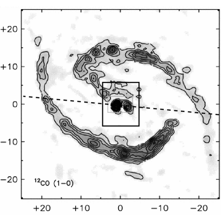
Figure 1: The field-of-view ($10.3\times 7.9$ arcsec) of the mosaicked GMOS IFU data is outlined (black rectangle) on a CO map (with the axes is arcsec) of the centre of NGC 1068 reproduced from Schinnerer et al. 2000. The CO map illustrates the central complexity in this galaxy with an inner spiral, an inner bar (PA$=48^{\circ}$) and a central CO ring. Also indicated is the position angle of the galaxy’s major axis (dashed line) at PA$=80^{\circ}$. At the assumed distance of 14.4 Mpc to NGC 1068, 1 arcsec corresponds to 70 pc.

In section 2, we give details of the observations and construction of the datacube. The datacube is analysed to decompose the emission lines into multiple components in Section 3, which also includes a brief examination of the main features that this reveals. In section 4, we use the stellar absorption features to constrain a model of the stellar disk and make associations between this and components in the emission line analysis.

2 Observations and Data Reduction

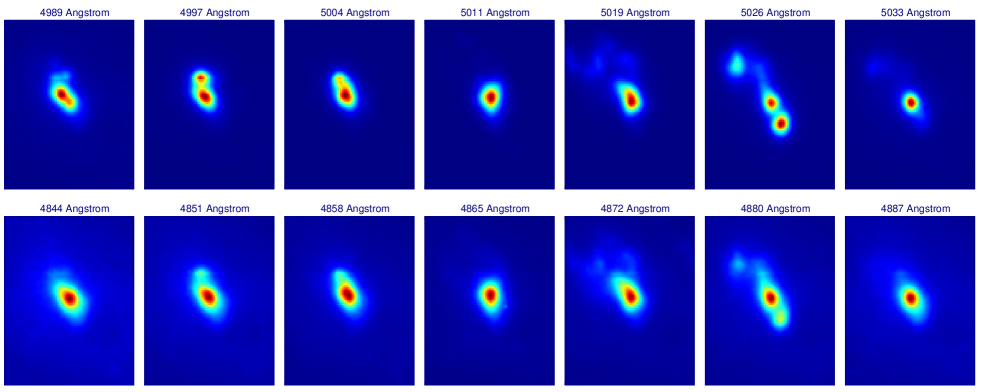
Figure 2: The top panels (each covering an area of 10.3 x 7.3 arcsec) show a series of one Angstrom wide wavelength slices through the data across the brightest [OIII] line. Across this line the central morphology of NGC 1068 develops various subcomponents. A similar change in morphology is witnessed across all other emission lines as illustrated by the next series of panels that show the emission distribution across the H$\beta$ line.

The GMOS IFU (Allington-Smith et al. 2002) is a fiber-lenslet system covering a field-of-view of $5\times 7$ arcsec with a spatial sampling of 0.2 arcsec. The IFU records 1000 contiguous spectra simultaneously and an additional 500 sky spectra in a secondary field located at 1.0 arcmin from the primary field.

The NGC 1068 observations on 9 Sep 2001 consist of 4 exposures of 900s. obtained with the B600 grating set to a central wavelength of 4900 Å and the $g^{\prime}$ filter (required to prevent overlaps in the spectra from each of the two pseudoslits into which the field is reformatted). The wavelength range in each spectrum was 4200 – 5400 Å. The seeing was  0.5 arcsec. Between exposures the telescope pointing was offset by a few arcsec to increase the covered area on the sky and to improve the spatial sampling. The pointing offsets from the centre of the GMOS field followed the sequence: (-1.75,+1.50), (-1.75,-3.00), (+3.50,+0.00), (+0.00,+3.00) arcsec.

The data were reduced using pre-release elements of the GMOS data reduction package (Miller et al. 2002 contains some descriptions of the IRAF scripts). This consisted of the following stages.

• Geometric rectification. This joins the three individual CCD exposure (each of $4608\times 2048$ pixels) into a single synthesised detector plane, applying rotations and offsets determined from calibration observations. At the same time, a global sensitivity correction is applied to allow for the different gain settings of the CCDs. Before this, the electronic bias was removed.

• Sensitivity correction. Exposures using continuum illumination provided by the Gemini GCAL calibration unit were processed as above. GCAL is designed to simulate the exit pupil of the telescope in order to remove calibration errors due to the illumination path. Residual large-scale errors were very small and were removed with the aid of twilight flatfield exposures. The mean spectral shape and the slit function (which includes the effect of vignetting along the direction of the pseudo-slit) were determined and used to generate a 2-D surface which was divided into the data to generate a sensitivity correction frame which removes both pixel-pixel variations in sensitivity, including those due to the different efficiencies of the fibres, and longer-scale vignetting loss in the spatial direction.

• Spectrum extraction. Using the continuum calibration exposures, the 1500 individual spectra were traced in dispersion across the synthesised detector plane. The trace coefficients were stored for application to the science exposures. Using these, the spectra were extracted by summing with interpolation in the spatial direction a number of pixels equal to the fibre pitch around the mean coordinate in the spatial direction. Although the spectra overlap at roughly the level of the spatial FWHM, resulting in cross-talk between adjacent fibres at the pseudoslit, the effect on spatial resolution is negligible since fibres which are adjacent at the slit are also adjacent in the field and the instrumental response of each spaxel is roughly constant. Furthermore it has no impact on the conditions for Nyquist sampling since this is determined at the IFU input (where $\geq 2$ spaxels samples the seeing disk FWHM) and not at the pseudo-slit. However the overlaps permit much more efficient utilisation of the available detector pixels resulting in a larger field of view for the same sampling (see Allington-Smith and Content 1998 for further details).

• Construction of the datacube. Spectra from the different pointings were assembled into individual datacubes. The spectra were first resampled onto a common linear wavelength scale using a dispersion relationship determined from 42-47 spectral features detected in a wavelength calibration observation. From the fitting residuals we estimate an RMS uncertainty in radial velocity of 8 km/s. The offsets between exposures were determined from the centroid of the bright point-like nucleus in each datacube, after summing in wavelength. The constituent datacubes were then co-added using interpolation onto a common spatial grid. The spatial increment was $0.1\times 0.1$ arcsec to minimise sampling noise due to both the hexagonal sampling pattern of the IFU and the offsets not being exact multiples of the IFU sampling increments. The resampling does not significantly degrade spatial resolution since the resampling increment is much smaller than the Nyquist limit of the IFU. Since the spectra had a common linear wavelength scale within each datacube, no resampling was required in the spectral domain. Cosmic ray events were removed by identifying pixels where the data value significantly exceeded that estimated from a fit to neighbouring pixels. The parameters of the program were set conservatively to avoid false detections. Since each spectrum spans $\sim$5 pixels along the slit, distinguishing single-pixel events such as cosmic rays from emission lines which affect the full spatial extent of the spectrum is quite simple. After this the exposures were checked by eye and a few obvious low-level events removed manually using local interpolation.

• Background subtraction. Spectra from the offset field were prepared in the same way as for the object field above, combined by averaging and used to subtract off the background sky signal. The sky lines were relatively weak in this observation so the accuracy of this procedure was not critical.

The result is a single merged, sky-subtracted datacube where the value at each point is proportional to the detected energy at a particular wavelength, $\lambda$, for a $0.1\times 0.1$ arcsec sample of sky at location $x,y$. The fully reduced and mosaicked NGC 1068 GMOS IFU data cube covers an area on the sky of $10.3\times 7.9$ arcsec with a spatial sampling of 0.1 arcsec per pixel and spectral resolving power of 2500. The wavelength range covered was 4170 – 5420 Å sampled at 0.456 Å intervals.

The change in atmospheric dispersion over the wavelength range studied is less than 1 spaxel so no correction has been applied. The spectra were not corrected to a scale of flux density since this was not required for subsequent analysis

3 Emission Line Data

The morphology of the central region changes rapidly across the emission lines. This is illustrated in Fig. 2 showing a series of monochromatic slices. The emission lines appear to consist of multiple components whose relative flux, dispersion and radial velocity change with position.

3.1 Empirical multi-component fits

To understand the velocity field of the line-emitting gas, we made multicomponent fits to the H$\beta$ emission line. This was chosen in preference to the brighter O[III] $\lambda\lambda$ 4959, 5007 doublet because of its relative isolation and because the signal/noise was sufficient for detailed analysis. The fits were performed on the spectra extracted for each spatial sample from the sky-subtracted and wavelength-calibrated datacube after it had been resampled to $0.2\times 0.2$ arcsec covering a field of $8.6\times 6$ arcsec and 4830 – 4920 Å in wavelength to isolate the H$\beta$ line. The resampling made the analysis easier by reducing the number of datapoints without loss of spatial information.

The continuum was found to be adequately fit by a linear function estimated from clean areas outside the line profile. A program was written to fit up to 6 Gaussian components, each characterised by its amplitude, $A$, radial velocity, $v$ and velocity dispersion, $\sigma$. The Downhill Simplex method of Nelder and Mead (1965) was used. This minimises $\chi^{2}$ evaluated as

$$\chi^{2}=\sum_{i=1}^{M}\left(\frac{F_{i}-f(x_{i};A_{i},\mu_{i},\sigma_{i}...A_{N},\mu_{N},\sigma_{N})}{s_{i}}\right)$$ (1)

where $F_{i}$ is the value of the $i$th datapoint. $M$ is the number of datapoints in the fit and

$$f(x_{i})=\sum_{j=1}^{N}A_{j}\exp\left[-\frac{(x_{i}-\mu_{j})^{2}}{2\sigma_{j}^{2}}\right]$$ (2)

is the sum of $N$ Gaussian functions. The radial velocity and velocity dispersion are determined from $\mu$ and $\sigma$ respectively. The noise, $s$, in data numbers was estimated empirically from the data as a sum of fixed and photon noise as

$$s_{i}=H\sqrt{\frac{F_{i}}{G}+s_{R}^{2}}$$ (3)

where the detector gain $G=2.337$ and the readout noise is $s_{R}=3.3$. The parameter $H=1.06$ represents the effect of unknown additional sources of error and was chosen to provide satisfactory values of $Q$ (see below) for what were judged by eye to be good fits.

The significance of the fit was assessed via $Q(\chi^{2}|\nu)$ which is the probability that $\chi^{2}$ for a correct model will exceed the measured $\chi^{2}$ by chance. The number of degrees of freedom, $\nu=M-3N$. $Q$ is evaluated as

$$Q(\chi^{2}|\nu)=Q(\nu/2,\chi^{2}/2)=\frac{1}{\Gamma(\nu/2)}\int^{\infty}_{\chi^{2}/2}\exp(-t)t^{\frac{\nu}{2}-1}dt$$ (4)

with limiting values $Q(0|\nu)=1$ and $Q(\infty|\nu)=0$.

Fits were attempted at each point in the field with $1\leq N\leq N_{\rm max}=6$, with $N$ increasing in unit steps until $Q\simeq 1.0$. The fits were additionally subject to various constraints to preclude unphysical or inherently unreliable fits, such as those with line width less than the instrumental dispersion ($\sigma<0.9$ pixels) or so large as to be confused with errors in the baseline subtraction ($\sigma>0.5M$ ). The final value of the fit significance (not always) unity was recorded as $Q_{\rm max}$. The fits at each datapoint were examined visually and in the small number of cases, where the fits were not satisfactory, a better fit was obtained with an initial choice of parameters chosen by the operator.

The uncertainty in the resulting radial velocities taking into account random and systematic calibration errors was estimated to be $\sigma=30\>{\rm km}\,{\rm s}^{-1}$. Examples of fits are shown in Fig. 3.

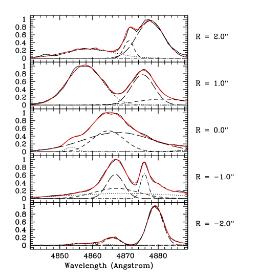
Figure 3: The normalized emission line profiles (black) obtained at various locations along a transect that coincides with the position angle of the jets. The individual Gaussian components whose sum best-fits the observed line profile are shown in different line styles. The red line shows the sum of the individual components.

The distribution of $Q_{\rm max}$ and $N_{\rm max}$ over the GMOS field-of-view suggests that most fits within the region of the source where the signal level is high are reliable but some points near the nucleus have lower reliability, perhaps because the required number of components exceeds $N_{\rm max}$. This is not surprising in regions where the signal/noise ratio is very high. There is a clear trend to greater numbers of components in the brighter (nuclear) regions of the object. This is likely to be due to the higher signal/noise in the brighter regions but may also reflect genuinely more complex kinematics in the nuclear region. An atlas of fits for each datapoint in the field of view with $N\geq 1$ is given in electronic form in the appendix.

3.2 Steps towards interpretation

Garcia-Lorenzo et al. (1999) and Emsellem et al. (2005) identified three distinct kinematical components in their [OIII] and H$\beta$ data based on line width. Our GMOS data obtained at a finer spatial and spectral resolution paints a considerably more complex picture. At even finer spatial resolution, HST spectroscopic data (e.g. Cecil et al. 2002; Groves et al. 2004) obtained with multiple longslit positions and narrow-band imaging adds further complexity, including features not seen in our data in which individual clouds can be identified and classified by their kinematics.

However, the HST longslit data must be interpreted with caution since it is not homogeneous in three dimensions and cannot be assembled reliably into a datacube. Making direct links between features seen in our data with those of these other authors is not simple, but subjective and ambiguous. This clearly illustrates how our understanding of even this accessible, archetypal galaxy is still strongly constrained by the available instrumentation despite recent major advances in integral-field spectroscopy and other 3D techniques.

The atlas of multicomponent fits to the emission line data provides a huge dataset for which many interpretations are possible. To indicate the complexity of the data, the line components along representative transects through the data are plotted in Figs. 4 & 5. The plots give the radial velocity for each fitted component as a function of distance along the transect as indicated on the white-light image obtained by summing over all wavelengths in the datacube. The component flux (the product of fitted FWHM and amplitude) is represented by the area of the plotted symbol and the FWHM is represented by its colour. H$\beta$ absorption is negligible compared to the emission and has been ignored in the fits.

Fig. 4 is for a “dog-leg” transect designed to encompass the major axis of the structure surrounding the brightest point in the continuum map (assumed to be the nucleus) and the bright region to the north-east. For comparison, Fig. 5 shows a transect along an axis roughly perpendicular to this. The following general points may be made from this:

Figure 4: A plot of radial velocity versus distance along the dog-leg NE-SW transect, as shown in the image, for each component fitted to the H$\beta$ line excluding uncertain fits. The change of direction marks the zero-point of the distance scale. The area of the circles is proportional to the component flux while the colour encodes the line width as indicated in the key. See the text for further details.

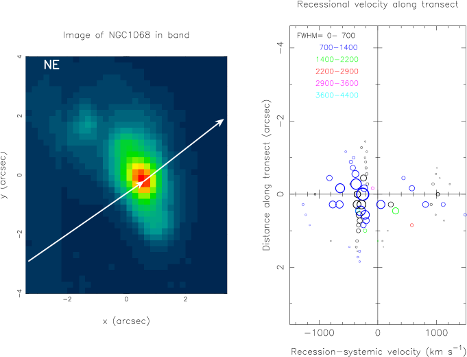
Figure 5: Same as the preceding figure but for a transect perpendicular to the previous one.

• Strong shears in radial velocity are present between north-east and south-west

• At each position along the transects there are a number of distinct components with different bulk radial velocity, spanning a large range ($\sim$3000 km/s)

• The majority of the observed flux comes from a component spanned by relative radial velocity –1000 km/s to 0 km/s

• This component, if interpreted as a rotation curve has a terminal velocity of $\pm$500 km/s, too large for disk rotation, so is more likely to indicate a biconical outflow with a bulk velocity that increases with distance from the nucleus, reaching an asymptotic absolute value of 500 km/s. This component also has a large dispersion which is greatest close to the nucleus.

• The closeness in radial velocity between components of modest dispersion within this structure (at transect distances between 0 and +1 arcsec) may arise from uncertainties in the decomposition of the line profiles into multiple components, i.e. two components of moderate dispersion are similar to one component with high dispersion,

• The other components are likely to indicate rotation of gas within disk-like structures, if the implied terminal velocities are small enough, or outflows or inflows.

• Any such flows do not appear to be symmetric about either the systemic radial velocity or the bulk of the emission close to the nucleus.

A comparison of the STIS [OIII] emission spectra along various slit positions (Cecil et al.; Groves et al.) provides qualitative agreement with our data in that most of the components in our datacube have analogues in their data. However their data suggest a much more clumpy distribution than ours, which is not surprising given the difference in spatial resolution. The apparently much greater range of radial velocity in their data is because our component maps indicate the centroid of the radial velocity of each component, not the full width of the line, which can be considerable (FWHM of 1000-2000 km/s). If we plot the line components in the same way as them, the dominant -1000 to 0 km/s component would fill in the range –2500 to +1000 in good agreement with their data.

There is evidence of a bulk biconic flow indicative of a jet directed in opposite directions from the nucleus plus a number of flows towards and away from the observer which could be either inflowing or outflowing, but which show a preference to be moving away from the observer. Some of these could be associated with disk-like components. As a first attempt towards interpretation, we seek to identify any gaseous components which can be associated with the stellar kinematics.

4 Absorption Line Data

4.1 Stellar Kinematics

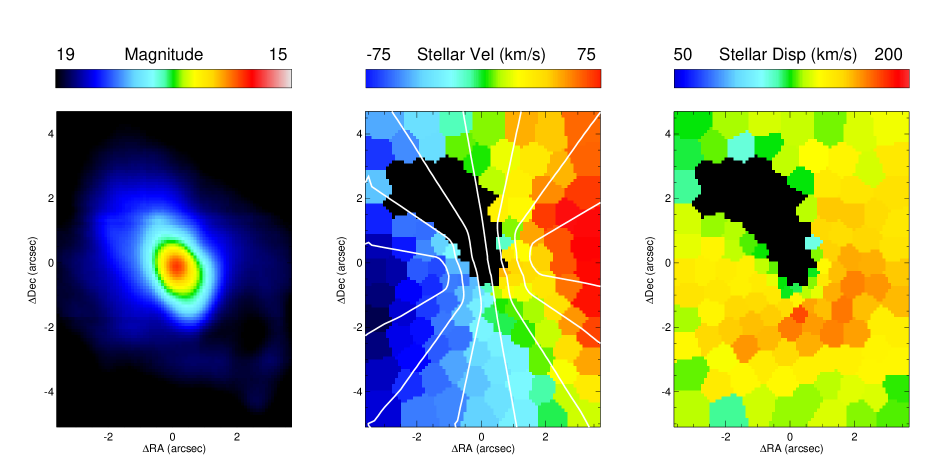
Figure 6: Maps of the stellar kinematics in the centre of NGC 1068. The reconstructed image (left panel) is obtained by summing all spectra in the GMOS IFU datacube from 5100 to 5400 Å. The magnitude scale has an arbitrary offset. The kinematical analysis presented in the next two panels uses data that are coadded into spatial bins with a signal-to-noise ratio of 20 or more using a Voronoi binning algorithm (Cappellari & Copin, 2003). The stellar velocity field (centre) and the stellar velocity dispersion (right panel) were derived by fitting a stellar template spectrum (type K0III) convolved with a Gaussian distribution to the spectral region around the Mg $b$ triplet ($\sim 5170$ Å). The systemic velocity has been subtracted in the central panel. The white contours in this panel show the best-fit model velocity field, see section 4.3. In all panels North is to the top and East is to the left. Blank regions indicate those areas where strong non-continuum emission prevented satisfactory fits to the absorption line data.

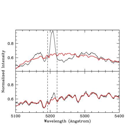
Figure 7: Two examples of stellar template fits (bold red lines) to absorption lines in the data cube. The top panel shows a spectrum from a location in the ‘wedge’ where strong non thermal emission significantly ‘eroded’ the absorption lines while the bottom panel shows a typical absorption line spectrum. In both panels the continuum is fit with a third order polynomial. A 6th order polynomial in the top panel would fit the continuum wiggles better but the derived kinematics are qualitatively similar to the 3rd order fit. The emission line in these panels is the [NI] line ($\lambda\lambda\ 5199.8$Å). The wavelength between the two dashed lines were excluded in the stellar template fits.

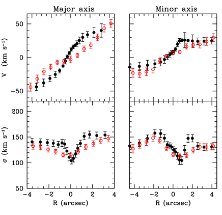
Figure 8: A comparison between the results derived from long-slit observations of Shapiro et al. (2003, open circles) and stellar kinematics derived from our GMOS data (filled circles). The long-slit results are obtained with the KPNO 4m telescope along the major axis (PA$=80^{\circ}$) and the minor axis (PA$=170^{\circ}$) of NGC 1068 (see Fig. 1). The slit width of 3.0 arcsec covers a substantial fraction of the GMOS observations. We mimic these long-slit observations by deriving the GMOS results in 3.0 arcsec wide cuts through the GMOS data. The differences between the two data sets are consistent with the effect of different PSFs.

Although the GMOS IFU commissioning observations of NGC 1068 concentrated on the bright emission lines, the Mg $b$ absorption line feature ($\sim 5170$ Å) is readily identifiable in the spectra over most of the field covered by these observations and can be used to derive the stellar kinematics. In order to minimize contamination by emission lines when extracting the stellar kinematics, we only used data in the wavelength range from 5150 to 5400 Å.

In order to reliably extract the stellar velocities from the absorption lines it is necessary to increase the signal-to-noise ratios by co-adding spectra. The $103\times 79$ individual spectra in the data cube were co-added using a Voronoi based binning algorithm (Cappellari & Copin 2003). While the improvement in signal/noise is at the expense of spatial resolution, the chosen algorithm is optimised to preserve the spatial structure of the target. A signal-to-noise ratio of $\gtrsim 20$ was used to bin the data, yielding 160 absorption line spectra above this threshold.

The stellar kinematics are extracted from these spectra using the standard stellar template fitting method. This method assumes that the observed galaxy spectra can be approximated by the spectrum of a typical star (the stellar template) convolved with a Gaussian profile that represents the velocity distribution along the line-of-sight. The Gaussian parameters that yield the smallest difference in $\chi^{2}$ between an observed galaxy spectrum and the convolved template spectrum are taken as an estimate of the stellar line-of-sight velocity and the line-of-sight stellar velocity dispersion. Various codes have been developed over the past decade that implement stellar template fitting. We have used the pixel fitting method of van der Marel (1994) in this paper.

Stellar template spectra were not obtained as part of the NGC 1068 GMOS IFU observations. Instead, we used a long-slit spectrum of the K0III star HD 55184 that was obtained with the KPNO 4m telescope in January 2002 on a run that measured the stellar kinematics along the major and minor axis of NGC 1068 (Shapiro et al. 2003). The instrumental resolution of the KPNO spectrum is the same as our GMOS data. Both the template spectrum and the GMOS IFU spectra were resampled to the same logarithmic wavelength scale before applying the kinematical analysis. The continuum in the galaxy spectra is handled by including a 3rd order polynomial in the fitting procedure.

The best-fit stellar velocities and stellar velocity dispersions are presented in Fig. 6. A section of the kinematical maps directly North East of the centre is empty. No acceptable stellar template fits could be obtained in this region (see also Fig. 7). The blank region lies along the direction of the approaching NE jet. Boosted non-continuum emission is therefore the most likely explanation for the observed blanketing of the absorption line features in this area.

4.2 Comparison and interpretation

Although part of the stellar velocity map is missing, the overall appearance is that of a regularly rotating stellar velocity field. The kinematical minor axis (with radial velocity, $v=0$) is aligned with the direction of the radio jets and with the long axis in the reconstructed GMOS IFU image. Garcia-Lorenzo et al. (1997) derive the stellar velocity field over the central $24\times 20$ arcsec in NGC 1068 from the Ca II triplet absorption lines. The part of their velocity map that corresponds to the GMOS IFU data is qualitatively consistent with our velocity map although there appears to be a rotational offset of about 15 degrees between the two velocity maps. Their best-fit kinematical major axis has PA$=88^{\circ}\pm 5^{\circ}$ while the GMOS IFU maps suggests PA $\simeq 105^{\circ}$. The latter is more consistent with the Schinnerer et al. (2000) best-fit major axis at PA$=100^{\circ}$.

In Fig. 8 we compare the GMOS data with results we derived from the long-slit data obtained along the (photometric) major and minor axes of NGC 1068 (Shapiro et al. 2003). The long-slit results were obtained from a 3.0 arcsec wide slit. The GMOS kinematics shown in this figure were therefore derived by mimicking the long-slit observations. That is, we extracted the kinematics from 3.0 arcsec wide cuts through the GMOS data along the same PAs as the long-slits. The long-slits partially overlap the wedge region seen in Fig. 6. However, because of the width of the mimicked slits, the contaminating effect of the centrally concentrated emission lines was significantly reduced. But some effects on the derived stellar kinematics remain. Most notably along the minor axis profiles at $\sim 2$ arcsec. (The Shapiro et al. results were obtained in fairly poor seeing conditions resulting in additional smearing.)

The stellar velocity dispersion map is missing the same region as the stellar velocity map. Although this includes the nucleus, it appears that the maximum velocity dispersion is located off-centre. The velocity dispersion profiles of NGC 1068 published in Shapiro et al. (2003) focused on the behaviour at large radii where contamination by emission lines is not an issue. A re-analysis of these data using a pixel based method rather than a Fourier based method shows that the velocity dispersions in NGC 1068 exhibit the same central drop (see also Emsellem et al. 2005) observed in the GMOS data. As the spectra of NGC 1068 show very strong emission lines in the central region of this system, the difference with the Shapiro et al. results can be attributed to unreliability of Fourier-based methods in the presence of significant emission lines.

Assuming that the velocity dispersions are distributed symmetrically around the major axis (PA$=100^{\circ}$) of the kinematical maps, the dispersion distribution resembles the dumbbell structures found in the velocity dispersion maps of the SABa type galaxy NGC 3623 (de Zeeuw et al. 2002) and the SB0 type galaxies NGC 3384 and NGC 4526 (Emsellem et al. 2004). A rotating (i.e. cold) disk embedded in a bulge naturally produces the observed dumbbell structure in the velocity dispersions. Both the position angle of the kinematical major axis and the orientation of the inferred nuclear disk are consistent with the central CO ring (diameter: 5 arcsec) identified by Schinnerer et al. (2000). Alternative interpretation of the incomplete NGC 1068 stellar dispersion map include a kinematically decoupled core or recent star formation (e.g. Emsellem et al. 2001). The GMOS stellar velocity maps compliment the larger scale maps of Emsellem et al. (2005) where the central structure (see their Fig. 6) becomes uncertain for the same reason as for the empty portion of our data.

4.3 A stellar disk model

Both the gas and stellar data present a very rich and complex morphology. As a first step toward interpretation we fit the GMOS stellar velocity map with a qualitative ‘toy’ model of a rotating disk. In a forthcoming paper, much more detailed and quantitative models of the gas and stellar data will be presented.

The disk model consists of an infinitely thin circular disk (in this simple model we use a constant density profile) with a rotation curve that rises linearly to $75\>{\rm km}\,{\rm s}^{-1}$ out a radius of 3 arcsec and thereafter remains constant. Both the best-fit amplitude and the break radius as well as the position angle of the disk model were found empirically by comparing the model velocity field to the GMOS velocity map in a least-square sense. We assumed that the disk is parallel to the plane of the galaxy (i.e. we assumed an inclination of $i=30$ degrees). The model velocity field is overplotted with white contours in the central panel of Fig. 6. The best-fit position angle of the disk model differs by some 30^∘ (PA${}_{\rm disk}=110^{\circ}$) from the major axis of NGC 1068 but is in close agreement with the kinematical position angle (e.g. Schinnerer et al. 2000).

A comparison between the disk model and the H$\beta$ data is shown in Fig. 9 at two different projections. The thin contours show the projected intensity distribution of H$\beta$ as a function of position and velocity. The projected intensity distribution of the disk model is overplotted as thick lines. In both panels the H$\beta$ distribution shows a spatially extended structure that is narrow in velocity space. The overplotted disk model closely matches the location and gradient of this structure in the data cube. To facilitate a comparison by eye the velocity distribution of the rotating disk model was broadened by $140\>{\rm km}\,{\rm s}^{-1}$, the mean observed velocity dispersion, in this figure. The most straightforward interpretation of this result is that part of the emission line distribution originates in a rotating gas disk that is aligned with the stellar disk in the centre of NGC 1068. This component can, with hindsight, clearly be seen in the transect maps (most evident in Fig. 4 near transect position $-4$ arcsec) as the aligned set of narrow components that are located closely to the systemic velocity of NGC 1068.

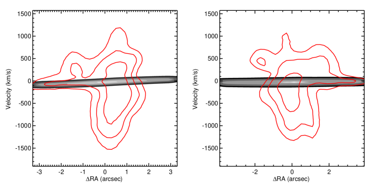
Figure 9: Comparison between the projected H$\beta$ flux distribution (thin lines) observed in the centre of NGC 1068 with the GMOS IFU and the projected density distribution of the disk model (thick shaded lines). In the left panel the data cube is collapsed along the declination axis, while the panel on the right shows the data cube collapsed along the RA axis. The disk-like structure in these data is clearly visible as the spatially extended, but narrow in velocity space, structure. The disk model closely matches both the location and the gradient of this structure.

5 Conclusions

We have used integral field spectroscopy to study the structure of the nucleus of NGC1068 at visible wavelengths. We present an atlas of multicomponent fits to the emission lines. Interpretation of this large, high-quality dataset is not straightforward, however, since the link between a given fitted line component and a real physical structure cannot be made with confidence. We have started our exploration of the structure by using absorption line data on the stellar kinematics in the disk to identify a similar component in the emission line data which presumably has its origin in gas associated with the disk. This analysis serves to illustrate both the complexity of the source and the enormous potential of integral-field spectroscopic data to understand it as well as the need for better visualization and analysis tools.

References

- (1) Allington-Smith, J. & Content, R. 1998. PASP 110, 1216-1234.
- (2) Allington-Smith, J., Murray, G., Content, R., Dodsworth, G., Davies, R., Miller, B. W., Jorgensen, I., Hook, I, Crampton, D., & Murowinski, R. 2002, PASP, 114, 892.
- (3) Antonucci, R. 1993, ARAA, 31, 473
- (4) Bacon, R., 2000. ’NGST Science and Technology Exposition’, ASP Conference Series, Vol. 207, p333, eds: E.P.Smith and K.S.Long.
- (5) Cappellari, M. & Copin, Y. 2003, MNRAS, 342, 345
- (6) Cecil, G., Bland, J., Tully, R. B. 1990, ApJ, 355, 70
- (7) Cecil, G., Dopita, M. A., Groves, B. A., Wilson, A.S., Ferruit, P., Pecontal, E., & Binette, L. 2002. ApJ 568, 627.
- (8) de Zeeuw, P. T., et al. 2002, MNRAS, 329, 513
- (9) Emsellem, E., Greusard, D., Combes, F., Friedli, D., Leon, S., Pecontal, E., & Wozniak, H. 2001, A&A, 368, 52
- (10) Emsellem, E., et al. 2004, MNRAS, 352, 721
- (11) Emsellem, E., Fathi, K., Wozniak, H., Ferruit, P., Mundell, C. G., & Schinnerer, E. 2005, A&A, in prep
- (12) Gallimore, J. F., Baum, S. A., O’Dea, C. P., & Pedlar, A. 1996, ApJ, 458, 136
- (13) Garcia-Lorenzo, B., Mediavilla, E., Arribas, S., & del Burgo, C. 1997, ApJ, 483, L99
- (14) Garcia-Lorenzo, B., Mediavilla, E., & Arribas, S. 1999, ApJ, 518, 190
- (15) Groves, B. A., Cecil, G., Ferruit, P., & Dopita, M. A. 2004. ApJ 611, 786.
- (16) Jaffe, W., et al. 2004, Nature, 429, 47
- (17) Krolik, J. H., & Begelman, M. C. 1988, ApJ, 329, 702
- (18) Macchetto, F., Capetti, A., Sparks, W. B., Axon, D. J., & Boksenberg, A. 1994, ApJ, 435, L15
- (19) Miller et al. 2002, ASP Conf. Ser. Vol. 288, p. 427.
- (20) Nelder, J.A. & Mead, R., The Computer Journal, 7, 308-313.
- (21) Peterson, B. M. 1997 ‘An introduction to AGN’, Cambridge University Press
- (22) Schinnerer, E., Eckart, A., Tacconi, L. J., & Genzel, R. 2000, ApJ, 533, 850
- (23) Scoville, N. Z., Matthews, K., Carico, D. P., & Sanders, D. B. 1988 ApJ, 327, L61
- (24) Shapiro, K. L., Gerssen, J., & van der Marel, R. P. 2003, AJ, 126, 2707
- (25) Thatte, N., Quirrenbach, A., Genzel, R., Maiolino, R., & Tecza, M. 1997, ApJ, 490, 246
- (26) Turner, J. 2001, PhD thesis, University of Durham.
- (27) van der Marel, R. P. 1994, MNRAS, 270, 271