Multi-spot ignition in type Ia supernova models

We present a systematic survey of the capabilities of type Ia supernova explosion models starting from a number of flame seeds distributed around the center of the white dwarf star. To this end we greatly improved the resolution of the numerical simulations in the initial stages. This novel numerical approach facilitates a detailed study of multi-spot ignition scenarios with up to hundreds of ignition sparks. Two-dimensional simulations are shown to be inappropriate to study the effects of initial flame configurations. Based on a set of three-dimensional models, we conclude that multi-spot ignition scenarios may improve type Ia supernova models towards better agreement with observations. The achievable effect reaches a maximum at a limited number of flame ignition kernels as shown by the numerical models and corroborated by a simple dimensional analysis. tars: supernovae: general – Hydrodynamics – Instabilities – Turbulence – Methods: numerical

1 Introduction

Over the past years, a consensus has emerged about the general astrophysical scenario of the majority of type Ia supernovae (SNe Ia). These events are associated with thermonuclear explosions of white dwarf (WD) stars close to the Chandrasekhar mass (for a recent review see Hillebrandt & Niemeyer, 2000). A thermonuclear flame ignited near the WD’s center is believed to propagate outward incinerating most parts of it. The released nuclear energy may suffice to explode the star as could be shown in several numerical simulations (e.g. Nomoto et al., 1984; Reinecke et al., 2002c; Gamezo et al., 2003; Röpke & Hillebrandt, 2005a).

Yet little is known about the way the thermonuclear flame ignites. The evolution towards flame ignition is a complex physical process. As a single WD is an inert object, dynamics must be introduced into the progenitor system by assuming it to be a binary. The favored scenario suggests a non-degenerate binary companion from which the WD accretes matter. Due to this mass accumulation it approaches the Chandrasekhar limit, steadily increasing its central density so that eventually carbon burning ignites. In the following several hundreds of years a simmering phase of convective burning sets the conditions under which finally a thermonuclear runaway occurs leading to the the formation of a flame. Unfortunately, the flame ignition is difficult to address both analytically and numerically. The few studies that tackled the pre-ignition evolution proposed different scenarios for flame formation. While one study claims the flame ignition to take place in only one single point near the center (Höflich & Stein, 2002), others favor an ignition in multiple sparks distributed around the center or on only one side of it, depending on the large-scale convective flow pattern (Garcia-Senz & Woosley, 1995; Woosley et al., 2004; Wunsch & Woosley, 2004; Iapichino, 2005).

Not being well constrained by theory, shape and location of the first flame(s) are usually treated as free initial parameters in multi-dimensional simulations. The hope was originally that those had only little impact on the models supporting the observational finding of a remarkable uniformity of SN Ia characteristics. However, multi-dimensional simulations starting with different initial flame configurations disagreed with this conjecture. The way of flame ignition turned out to be one of the influential parameters of the models. Different choices gave rise to controversial results. Single-spot central ignitions leading to explosions of the WD were studied by Niemeyer & Hillebrandt (1995), Reinecke et al. (1999a), Hillebrandt et al. (2000), Reinecke et al. (2002a), Reinecke et al. (2002c), and Gamezo et al. (2003). In contrast, off-center single-spot ignitions release insufficient energy to explode the star (Niemeyer et al., 1996; Calder et al., 2004). Multi-spot ignition scenarios were applied by Niemeyer et al. (1996), Reinecke et al. (2002b), and Röpke & Hillebrandt (2005a) and seem to have the potential to increase the explosion strength. Apparently, a slight misalignment of the initial flame with the WD’s center leads to a drastic change in the outcome of the simulations when starting with a single perfect sphere (Calder et al., 2004). More structured multi-spot flame configurations are less sensitive to it (Röpke & Hillebrandt, 2005a). But even setting aside the complications arising from asymmetries in off-center ignitions, the results of the models have been shown to depend on the number of flame seeds (Reinecke et al., 2002b; Travaglio et al., 2004). The objective of the present study is to explore this effect in detail in a systematic approach.

The question of what can be expected from multi-spot ignition scenarios with an increasing number and different distributions of initial flames was addressed only recently by García-Senz & Bravo (2005). We report on a similar study, which is, however, based on a completely different approach to modeling thermonuclear supernovae. While García-Senz & Bravo (2005) apply a Lagrangian description of the hydrodynamics based on the smooth particle hydrodynamics (SPH) technique, we utilize an Eulerian grid-based finite volume method. The key distinction is that our approach facilitates a self-consistent description of turbulent thermonuclear flame propagation, as will be discussed in Sect. 3. In contrast, the SPH model has to rely on a parameterization of the effective turbulent flame propagation velocity, since it cannot provide a valid description of turbulence effects. The predictive power of the SPH approach is thus limited. Nevertheless, the large-scale structures observed by García-Senz & Bravo (2005) appear to be similar to what we find in our simulations, as can be seen from a comparison with a full-star model presented by Röpke & Hillebrandt (2005a). This is not too surprising since both are driven by buoyancy and should be equally well reproduced in both approaches.

As will be discussed below, the simulation parameters and the details of the results of the present study differ significantly from those of García-Senz & Bravo (2005). Moreover, the focuses of the two surveys are distinct. While García-Senz & Bravo (2005) presented the first attempt to modeling SNe Ia in three dimensions (albeit in a parametrized way) from flame formation on and to assess the resulting explosions, we take a more pragmatic point of view. Our objective is to answer the question whether multi-spot ignition scenarios are in principle capable of curing some of the shortcomings of current deflagration SN Ia models. We therefore apply a number of different initial flame configurations without attempting to model their pre-ignition evolution. The question of how realistic these are is set aside in the present study.

Although being within the range of observational expectations, the explosion energies and the masses of burning products in all multi-dimensional deflagration models presented so far seem to be on the weak side and multi-spot ignition scenarios may offer a way to improve the results. Besides such global quantities, we are especially interested in the distribution of the species in velocity space. Previous work showed that poorly resolved models are inconsistent with observations in predicting low-velocity oxygen and carbon lines in late time spectra (Kozma et al., 2005). This is due to downdrafts of unburnt material in between burning buoyancy-driven bubbles of ashes. These downdrafts transport significant amounts of carbon and oxygen towards the center of the WD. It may well be, however, that the downdrafts carry sparks seeding additional burning, which are not resolved in current simulations. Moreover, the simulation from which the synthetic spectrum of Kozma et al. (2005) was derived started out with a very artificial initial central flame configuration. The model was calculated on a uniform computational grid of $[256]^{3}$ cells co-expanding with the WD. This led to an only marginally converged result and the explosion energy as well as the production of iron group and intermediate mass elements was rather low. Obviously, some of the disagreements with the observations are caused by the simplicity of the model – in particular the initial flame shape – and one may wonder whether the problems are mitigated with more structured flame configurations such as arising from multi-spot ignition.

An estimate of the capabilities of the multi-spot ignition scenario is given in Sect. 2. In Sect. 3 we will briefly outline the techniques underlying our numerical simulations and discuss a new implementation that enables us to study multi-spot ignition scenarios in detail. This implementation is compared with previous simulations in Sect. 4. Results from two-dimensional models will be discussed in Sect. 5. Although it will be shown that these are inappropriate to study multi-spot ignitions, they point to important effects. A systematic survey based on three-dimensional simulations is presented in Sect. 6. In Sect. 7 we draw conclusions for modeling thermonuclear supernova explosions.

2 Multi-spot ignition: estimating the gains

Woosley et al. (2004) and Wunsch & Woosley (2004) conclude from analytical models of the ignition process that a multi-spot ignition is possible (but not guaranteed). Timescale arguments show that a number of hot spots is in principle capable of evolving towards a thermonuclear runaway. The first flame will ignite at a radius $\sim$$150\,\mathrm{km}$ off-center of the WD and more can follow. Yet their number and spatial distribution cannot be conclusively constrained by the analytical models.

Thus, it is justified to regard these as free parameters in simulations of the explosion process. In this spirit, we address the question of the number of ignition spots in the present study. Concerning the spatial distribution we simplify matters by assuming a spherically symmetric probability density of ignitions to occur around the WD’s center. This ignores possible large-scale anisotropies of the ignition process due to low-order modes in the convective flow pattern prior to ignition (Woosley et al., 2004). The impact of such effects is subject to a forthcoming publication.

Given the ambivalence of the ignition conditions, it is a legitimate question to ask which multi-spot configuration would lead to an optimal fuel consumption producing the most vigorous explosion and potentially burning most of the fuel near the center. A dimensional analysis such as presented in the following can shed some light on this issue. Sects. 5 and 6 will tackle the question from the side of numerical simulations.

One has to note that there are two major effects on the outcome of multi-spot ignitited supernova simulations. If a single flame seed is separated from the bulk of ignition sparks towards larger radii, it will experience a larger gravitational acceleration. The burning front resulting from this spark will evolve faster than the other ignition points and dominate the flame evolution. This effect is determined by the nonlinear evolution of the burning fronts and hard to predict analytically. It will thus be discussed on the basis of numerical simulations in Sects. 5 and 6. Here, we only note that the distribution of ignition points should not be too sparse in order to avoid such effects.

On the other hand, accomodating too many ignition kernels in a given volume will have the effect that the flames merge shortly after ignition due to self-propagation. In this case, the simulation will look similar to those ignited centrally in a single connected shape. The main advantage of multi-spot ignition scenarios, i.e. a large flame surface, is lost. Two effects counteract the surface distruction by merging of the fronts. Firstly, the overall expansion of the star due to the nuclear energy release leads to an increasing separation of burning bubbles and, secondly, buoyancy-induced flotation rises them in radial direction further increasing their separation.

In a simplified picture, two igniting bubbles of radius $r_{\mathrm{b}}$ at a separation $l$ will lead to a maximum flame surface if their growth due to flame propagation is exactly compensated by these two effects. Assuming a homologous expansion of the star, the temporal change in distance of the bubbles, $\dot{l}_{\mathrm{ex}}$ induced by this effect is given by

$$\frac{l-2r_{\mathrm{b}}}{\dot{l}_{\mathrm{ex}}}=\tau_{\mathrm{dyn}},$$ (1)

where $\tau_{\mathrm{dyn}}\sim(G\rho)^{-1/2}=0.07\,\mathrm{s}$ is the dynamical timescale assuming a density of $3\times 10^{9}\,\mathrm{g}\,\mathrm{cm}^{-3}$ ($G$ denotes Newton’s constant).

Due to buoyancy, two neighboring bubbles enclosing an angle $\phi$ with the star’s center will rise radially, increasing their separation by

$$\dot{l}_{\mathrm{buoy}}=2\dot{r}\sin\frac{\phi}{2}.$$ (2)

For the angle $\phi$ we assume

$$\sin\frac{\phi}{2}=\frac{l-2r_{\mathrm{b}}}{2\langle r\rangle},$$ (3)

with an average initial distance $\langle r\rangle$ of the bubbles from the WD’s center. Thus,

$$\dot{l}_{\mathrm{buoy}}=\dot{r}\frac{l-2r_{\mathrm{b}}}{\langle r\rangle}$$ (4)

The asymptotic radial rise velocity of a bubble is (up to a factor of order unity) given by

$$\dot{r}=\sqrt{\mathrm{At}\,g\,r_{\mathrm{b}}}$$ (5)

(Davies & Taylor, 1950), where $\mathrm{At}=(\rho_{\mathrm{u}}-\rho_{\mathrm{b}})/(\rho_{\mathrm{u}}+\rho_{\mathrm{b}})$ denotes the Atwood number across the flame front with the density $\rho_{\mathrm{u}}$ of unburnt material outside and the density $\rho_{\mathrm{b}}$ of the burnt material inside the bubble. In its functional form, Eq. (5) follows the expression obtained from balancing the buoyancy and the drag forces for a spherical bubble. Typical values are $g\sim 10^{9}\,\mathrm{cm}\,\mathrm{s}^{-2}$ and about 0.07 for the Atwood number at a fuel density of $\rho_{\mathrm{b}}\sim 3\times 10^{9}\,\mathrm{g}\,\mathrm{cm}^{-3}$(Timmes & Woosley, 1992).

The distance decrement by growth of the bubbles due to burning is given by the propagation velocity of the flame front,

$$\dot{l}_{\mathrm{burn}}=2v_{\mathrm{burn}},$$ (6)

with $v_{\mathrm{burn}}\sim 10^{7}\,\mathrm{cm}\,\mathrm{s}^{-1}$ shortly after ignition. Equating the sum of $\dot{l}_{\mathrm{ex}}$ and $\dot{l}_{\mathrm{buoy}}$ with $\dot{l}_{\mathrm{burn}}$ yields for the optimal initial bubble separation $l_{\mathrm{opt}}$

$$l_{\mathrm{opt}}-2r_{\mathrm{b}}=\frac{2v_{\mathrm{burn}}\tau_{\mathrm{dyn}}\langle r\rangle}{\langle r\rangle+\tau_{\mathrm{dyn}}\sqrt{\mathrm{At}\,g\,r_{\mathrm{b}}}}.$$ (7)

The average density of bubbles $n$ in a sphere of radius $R$ is given by

$$n=\frac{3N}{4\pi R^{3}},$$ (8)

with $N$ denoting the number of bubbles. In the optimal case, this should be equal to the inverse volume of a sphere with radius $0.5l_{\mathrm{opt}}+r_{\mathrm{b}}$, i.e. the number of bubbles in this case is given by

$$N_{\mathrm{opt}}=\left\{\frac{R\,\left(\langle r\rangle+\tau_{\mathrm{dyn}}\sqrt{\mathrm{At}\,g\,r_{\mathrm{b}}}\right)}{\tau_{\mathrm{dyn}}v_{\mathrm{burn}}\langle r\rangle+2r_{\mathrm{b}}\langle r\rangle+2\tau_{\mathrm{dyn}}r_{\mathrm{b}}\sqrt{\mathrm{At}\,g\,r_{\mathrm{b}}}}\right\}^{3}.$$ (9)

Thus, assuming a central density of the WD of $3\times 10^{9}\,\mathrm{g}\,\mathrm{cm}^{-3}$, an ignition radius of 100 to 150$\,\mathrm{km}$ (Woosley et al., 2004), and setting the average initial distance from the center $\langle r\rangle$ to one half of this radius, the optimal number of ignition sparks with a radius of $r_{\mathrm{b}}=5.5\,\mathrm{km}$ (being the smallest resolvable bubble structure in the numerical models discussed below) should be somewhere between 23 and 76 per octant. This, of course, is no more than a crude estimate. Due to burning the bubbles will increase in size and this in turn affects the energy release and the contribution from buoyancy effects. Moreover, the establishing flows and the interaction of the flame with turbulence have been ignored. In a realistic numerical simulation, the flame seed configuration is much more complex. In most setups (see Sects. 5 and 6) we will apply a Gaussian distribution in radius. Since the outer bubbles are more separated in this case, the optimal number of bubbles is expected to be larger than the simple estimate.

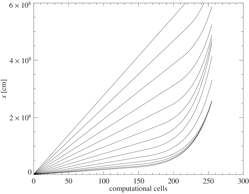
Figure 1: Evolution of the hybrid computational grid in a three-dimensional simulation. Each curve corresponds to a time progression of $\Delta t=0.1\,\mathrm{s}$, starting at the lowest curve with $t=0\,\mathrm{s}$.

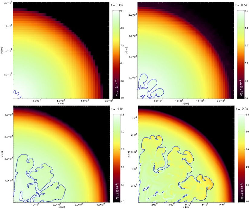
Figure 2: Snapshots of the evolution of a c3-model on a $256^{2}$ cells hybrid grid. The logarithm of the density is color-coded and the contour marks the location of the flame front.

With Eq. (9) the question can be answered of whether it is possible to tune models to give more vigorous explosions by increasing the resolution and accommodating an ever larger number of ignition spots. Even in the limit of $r_{\mathrm{b}}\rightarrow 0$ the optimal number $N_{\mathrm{opt}}$ of flame seeds increases to no more than 354 to 1195 per octant. Thus the effect of the number of initial flame sparks on the explosion strength is limited.

3 Explosion: astrophysical scenario and numerical methods

The explosion model describes the propagation of the flame after ignition near the center of the WD outwards. Our implementation is based on the deflagration scenario in which the flame velocity is sub-sonic and accelerated by the interaction with turbulence generated by generic instabilities (see e.g. Hillebrandt & Niemeyer, 2000). It follows the numerical methods developed by Reinecke et al. (1999b, 2002a) and Röpke (2005). For the details and extensive tests of the implementation we refer to these works. The fundamental concept behind the approach is that of large eddy simulations (LES). Only the largest scales of the problem are directly resolved. The interaction of the flame with turbulent eddies on unresolved scales of the establishing turbulent energy cascade is described by a sub-grid scale turbulence model (Niemeyer & Hillebrandt, 1995). The large separation of the flame width (of the order of a millimeter) from the resolved scales justifies the flame modeling as a sharp discontinuity separating the fuel from the ashes. To this end, the level-set technique is applied as described in detail by Reinecke et al. (1999b).

We apply the same WD equation of state as used by Reinecke et al. (2002a). In all simulations presented in the present paper we fix the initial composition to equal parts of carbon and oxygen throughout the star and construct the initial WD assuming cold isothermal ($T=5\times 10^{5}\,\mathrm{K}$) conditions and a central density of $2.9\times 10^{9}\,\mathrm{g}\,\mathrm{cm}^{-3}$. The nuclear reactions are implemented in the simplified approach suggested by Reinecke et al. (2002a). Five species (¹²C, ¹⁶O, ²⁴Mg representing the intermediate mass elements, ⁵⁶Ni as a representative of the iron group, and $\alpha$-particles) are followed. At high fuel densities the material crossed by the flame is converted to nuclear statistical equilibrium modeled as a mixture of “Ni” and $\alpha$-particles. Below fuel densities of $5.25\times 10^{7}\,\mathrm{g}\,\mathrm{cm}^{-3}$ intermediate mass elements are produced and once the fuel density drops below $10^{7}\,\mathrm{g}\,\mathrm{cm}^{-3}$ we stop burning. In the current implementation electron captures are neglected. These could decrease the density in the ashes and therefore increase the density contrast over the flame. In the setups chosen for our simulations we expect the effect on the dynamics of the explosion to be small, but significant changes may result at still higher central densities than those applied here.

Our novel approach that enables us to study the effects of initial flame configurations in detail is a computational grid different from previous implementations. While the first three-dimensional simulations by Hillebrandt et al. (2000) and Reinecke et al. (2002a, b, c) were carried out on static Cartesian grid geometries with a fine-resolved uniform inner part and an exponentially growing grid spacing further out to capture parts of the expansion in the explosion process, Röpke (2005) and Röpke & Hillebrandt (2005a) applied a moving uniform grid that tracked the expansion of the WD star. Here, we combine both approaches and use a moving grid that is composed of two nested sub-grids. The inner part (grid 1) again features a uniform fine resolution and the outer grid cells (grid 2) grow exponentially. Initially, both grids are moved individually. While grid 1 contains the flame and tracks its propagation, grid 2 follows the WD expansion. Since in the course of the explosion the flame spreads out over the WD star, grid 1 must expand faster than grid 2. It is therefore possible to subsequently gather cells of grid 2 into grid 1 as soon as the grid spacings match. Eventually, grid 1 incorporates grid 2 and the full WD is covered by a single uniform grid tracking its expansion. We will call this approach hybrid grid in the following. An example for the grid evolution in one of our simulations is given in Fig. 1.

Although conceptually simple, the hybrid grid has proven to be extremely useful and is much easier to handle than adaptive mesh refinement strategies. Since the expansion and flame spread in the explosion is on average spherical for most ignitions scenarios, it offers the possibility to maximally resolve the flame region with a given fixed number of computational cells. This leads to an improved modeling of the flame propagation and, in particular, provides the possibility to drastically improve the resolution in the central parts at the onset of the explosion. In this way it becomes feasible to resolve highly structured initial flame configurations. For studying multi-spot ignition scenarios, the number of initial flame kernels could be substantially increased. Whereas the previous static grid setups of one octant of the WD star could resolve up to $\sim$30 bubbles in a simulation with $768^{3}$ grid cells (cf. Travaglio et al., 2004), a hybrid-grid setup with $256^{3}$ cells can accommodate several hundreds of ignition spots.

All simulations performed in this study are carried out on only one spatial octant of the WD assuming mirror symmetry to the other octants. As demonstrated by Röpke & Hillebrandt (2005a), this symmetry constraint does not suppress a development of potential low-wavenumber modes in the nonlinear flow pattern. Although these may in principle occur in convective phenomena, the short explosion time-scale in SNe Ia prevents them. Therefore restricting the simulations to only one octant does not miss physical effects and provides a valid approach to save computer time in our study.

4 Testing the implementation

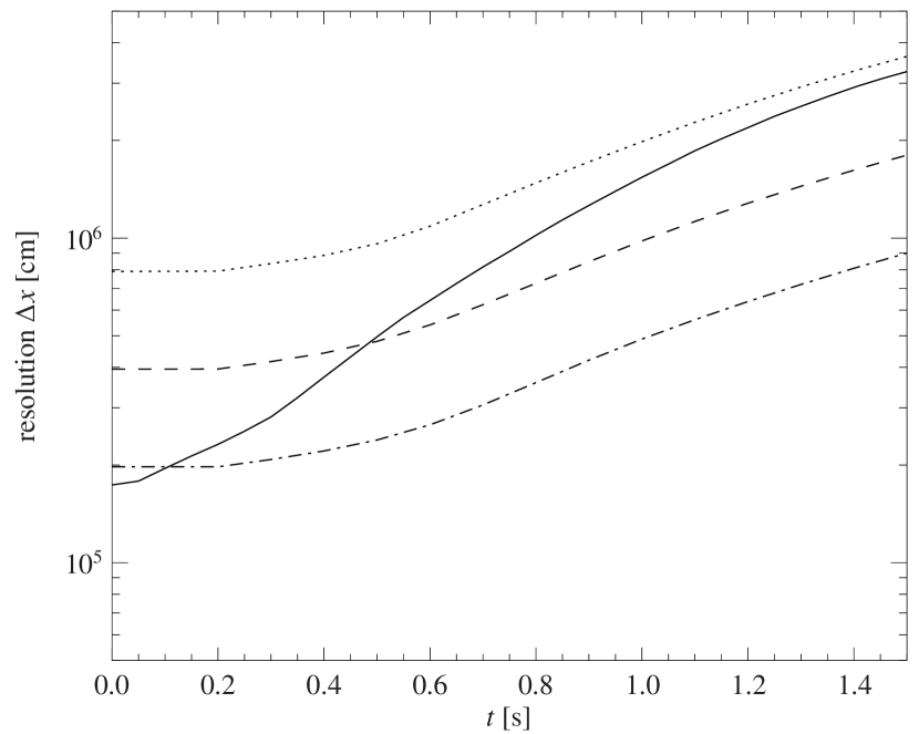
Figure 3: Flame resolution in different simulations: $256^{2}$cells hybrid grid (solid), $256^{2}$cells uniform grid (dotted), $512^{2}$cells uniform grid (dashed), and $1024^{2}$cells uniform grid (dashed-dotted).

Apart from a better resolution of the ignition, our approach concentrates resolution in the flame region also in the subsequent stages of the explosion. It is therefore worthwhile to compare the results with previous simulations. In particular, we will point out some changes with respect to the expanding uniform grid simulations of Röpke (2005). For this comparison, we apply the standard test case of a single-octant simulation in which the flame is centrally ignited with a sinusoidal (2d) or toroidal (3d) perturbation imposed on it. According to the notation of Reinecke et al. (2002a), we will refer to this flame setup as c3.

Figure 2 shows snapshots from the evolution of a c3-model in two dimensions imposing cylindrical symmetry. Here, a $256^{2}$ cells hybrid grid was applied. The initial c3 flame is depicted in the upper left panel of Fig. 2. Comparing these snapshots to those of the previous uniform-grid implementations (cf. Fig. 4 of Röpke, 2005), we note that the global structure resembles the simulations there carried out on a much larger number of computational cells. These, however, possess finer sub-structures. The reason is clear from a comparison of the resolutions of the flame fronts in the different implementations provided by Fig. 3. Due to the moving grids the resolution changes with time in all cases. As expected, the concentration of computational cells in the flame part leads to a much better resolution of the flame in the first stages for the hybrid implementation on $256^{2}$ cells than for the uniformly expanding $256^{2}$ cells grid. It is similar to the uniformly expanding $1024^{2}$ cells grid implementation. Therefore, the large-scale structures, seeded by the initial c3 flame perturbations evolve in a balanced way, whereas in the older implementation with $256^{2}$ grid cells the inner Rayleigh-Taylor finger was suppressed (cf. Fig. 4 of Röpke, 2005). Since the flame propagates faster than the WD expands, the resolution in later stages – when the two nested grids have evolved into a single uniform grid – converges towards that of the previous implementation. Naturally, this prevents the flame from developing as detailed fine structures as the uniform grid $1024^{2}$ implementation. This effect is, however, compensated with regard to the global quantities by the sub-grid scale turbulence model. We conclude that our novel implementation provides a reasonable compromise between computational expenses from larger grids and resolution of the flame.

The situation is very similar in three-dimensional simulations. A snapshot from the standard c3_3d model $1.0\,\mathrm{s}$ after ignition is shown in Fig. 4. As in the two-dimensional case, the three-dimensional implementation of the hybrid grid leads to a more balanced evolution of the flame morphology imprinted on the initial flame seed. The c3_3d model in previous uniform grid implementations (see Fig. 13 of Röpke, 2005) showed three strong flame features evolving along the axes due to a suppression of initial perturbations. This grid-imprinted symmetry is relaxed in the novel implementation in which the flame is structured into more and smaller features (see Fig. 4). Interestingly, the energy production is not increased by these effects in the three-dimensional simulations (cf. the energy release of the c3_3d model on a uniform expanding grid presented by Röpke, 2005), corroborating the conclusion that the description of the burning (at least in the stages where it proceeds to iron group elements) is numerically converged in our models. Although increased resolutions give rise to a modified structure of the flame and a redistribution of the ashes, the global quantities are largely unaffected.

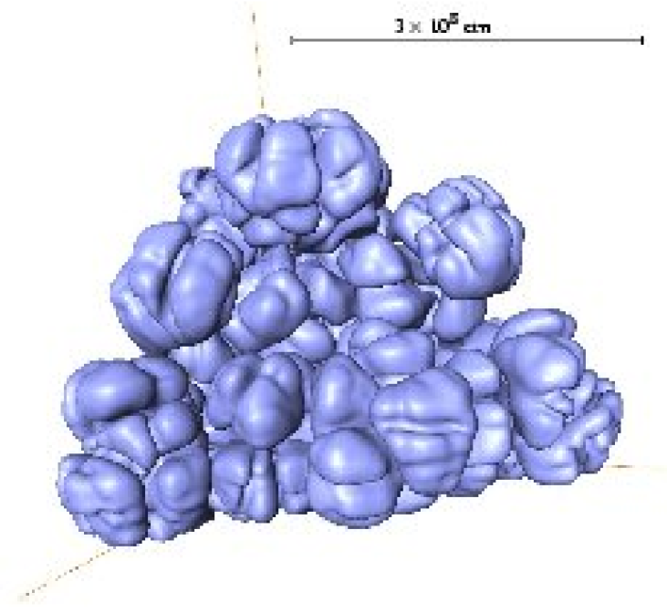
Figure 4: Flame front in model c3_3d $1.0\,\mathrm{s}$ after ignition.

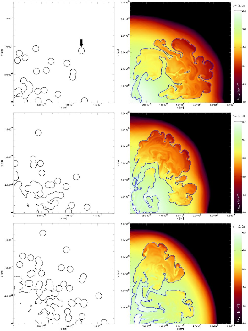
Figure 5: Two-dimensional multi-spot simulations: model b30_2d (top), model b100_2d (middle), and model b200_2d (bottom). The left column shows the initial flame configuration and the right column provides snapshots of the evolution after $2\,\mathrm{s}$ with the the logarithm of the density color-coded and the flame front represented by the contour. The arrow in the top left panel marks the bubble that later on dominates the flame evolution.

5 Two-dimensional simulations

With the hybrid grid implementation, four different flame configurations were tested in two-dimensional simulations again assuming a cylindrical symmetry. All were carried out on $256^{3}$ grid cells with an initial inner grid spacing of $1.74\,\mathrm{km}$. Apart from the c3_2d-model, different numbers of initial bubbles were chosen in the following procedure. The bubbles with a radius of $5.5\,\mathrm{km}$ were distributed randomly in angle and according to a Gaussian probability distribution with a dispersion of $\sigma=75\,\mathrm{km}$ in radius. This Gaussian radial distribution, however, was distorted by the constraint that no bubble was allowed to ignite at a radius larger than $2.5\sigma$ and by imposing a minimum distance of the bubble centers $d_{\mathrm{min}}$. The models b30_2d, b100_2d, and b200_2d contained 30 bubbles with $d_{\mathrm{min}}=0.8$, 100 bubbles with $d_{\mathrm{min}}=0.2$, and 200 bubbles with $d_{\mathrm{min}}=0.1$, respectively.

The initial flame configurations are shown in Fig. 5. This figure also contains snapshots at $t=2\,\mathrm{s}$. From a comparison with the c3_2d-model in Fig. 2 it is clear that in the two-dimensional case multi-spot ignition scenarios do not give rise to an increased overall fuel consumption. This is confirmed by the evolution of the total energies in the different models plotted in Fig. 6. The models b30_2d and b100_2d produce only about 40% of the asymptotic kinetic energy of model c3_3d and the energy production of model b200_2d falls in between.

The reason for this finding is a peculiarity of two-dimensional models. Apart from the fact that turbulence in the two-dimensional case follows a different scaling than three-dimensional turbulence, two-dimensional simulations tend to amplify large structures. This may be attributed to the missing degree of freedom in the third spatial direction where axial symmetry is imposed. Thus the initial flames consist of tori rather than bubbles. The large-scale flows around these structures are expected to significantly differ from the flow patterns in three-dimensional simulations.

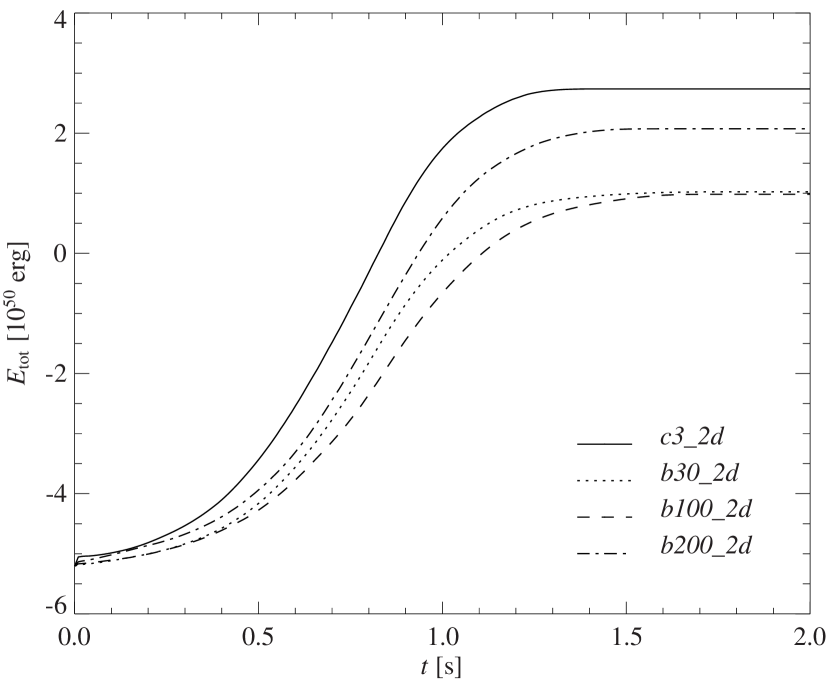
Figure 6: Total energies in the two-dimensional simulations.

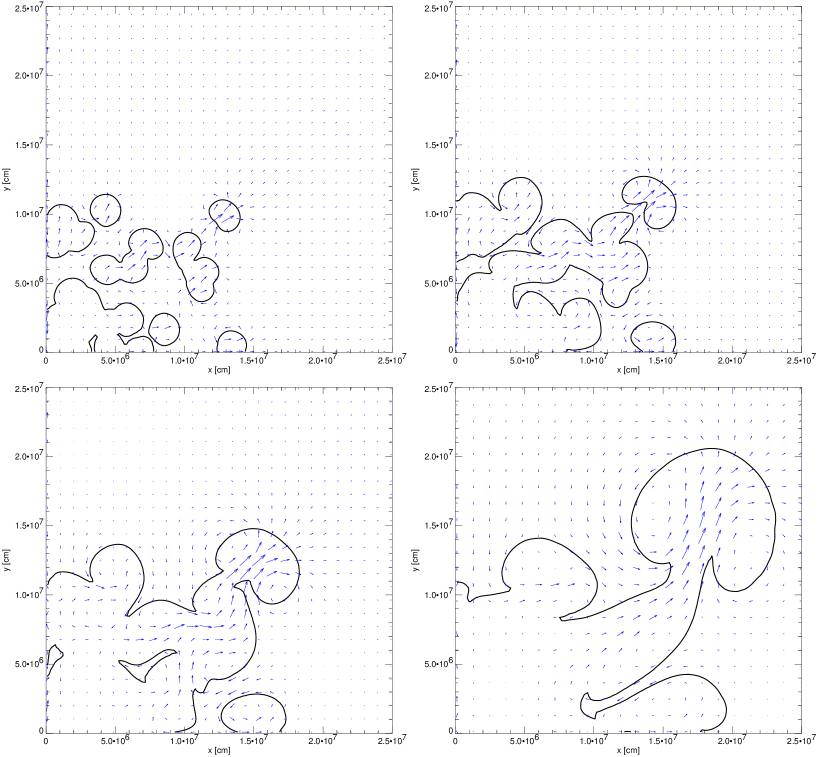
Figure 7: Flame evolution and velocity fields in model b30_2d at $t=0.05\,\mathrm{s}$, $t=0.10\,\mathrm{s}$,$t=0.15\,\mathrm{s}$, and $t=0.25\,\mathrm{s}$ (top left to bottom right).

As a result, in cases with few ignition spots, the outermost flame seed dominates the evolution. This is illustrated by snapshots of the early flame evolution in model b30_2d in Fig. 7. Starting from the initial configuration shown in Fig. 5, the inner flames merge quickly, but the outermost ignition spot (marked with the arrow in Fig. 5) evolves into a structure that dominates the flame evolution further on (cf. the snapshots in Fig. 7 and the snapshot at $t=2\,\mathrm{s}$ in Fig. 5). A similar effect governs the flame evolution in model b100_2d. Due to the larger number of ignition spots in model b200_2d the flame propagation is more balanced here and finally becomes dominated by two large features (see Fig. 5). The reason why the c3_2d-model appears so well-behaved is the symmetric and balanced perturbation we impose on the initial flame. It imprints three features which evolve equally.

Our results are in reasonable agreement with the findings of Niemeyer et al. (1996) and the recent study by Livne et al. (2005), both reporting on dominating large-scale flame features.

Thus our findings point to the effect mentioned in Sect. 2. Single spots may lead to large-scale features which have an unfavorable effect on the burning. Since flow patterns in two-dimensional simulations differ significantly from those in three-dimensional cases, the question arises of how pronounced this effect is there.

6 Three-dimensional simulations

6.1 Ignition setups

With the three-dimensional implementation of our scheme, we performed seven simulations with different initial flame configurations. The three-dimensional analog of our standard test model c3_2d, termed c3_3d, served as comparison with two-dimensional runs and with previous three-dimensional setups on other grid geometries. Five ignition configurations with bubbles of a radius of $5.5\,\mathrm{km}$ were chosen in a similar way as the setups for the two-dimensional simulations of Sect. 5. Again, a Gaussian radial distribution was applied, with a dispersion of $\sigma=75\,\mathrm{km}$. According to the number of igniting bubbles, the models are denoted as b15_3d, b30_3d, b55_3d, b150_3d, and b250_3d. In yet another setup, b500_3d, we assumed an equipartition over the radius instead of a Gaussian distribution. The models are summarized in Table 1 and the distributions of the ignition kernels in the multi-spot scenarios are depicted in the left columns of Figs. 9 and 10. Potentially, the maximum distance of flame ignition is a relevant parameter since the gravitational acceleration increases steeply in the inner part of the WD. The values of the maximal ignition radii are given in Table 1. Fig. 8 shows the energetic evolution of the models.

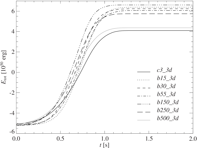
Figure 8: Total energies in the three-dimensional simulations.

Table 1: Flame configurations and results of three-dimensional models.

model	number of ignition spots	max. ignition radius $[10^{7}\,\mathrm{cm}]$	$M$(“Ni”) $[M_{\odot}]$	$M$(“Mg”) $[M_{\odot}]$	$M$(C,O) $[M_{\odot}]$	$E_{nuc}$ $[10^{51}\,\mathrm{erg}]$	$E_{tot}$ $[10^{50}\,\mathrm{erg}]$
c3_3d	(1)	1.80	0.511	0.157	0.738	0.93	4.27
b15_3d	15	1.68	0.657	0.158	0.591	1.16	6.62
b30_3d	30	1.69	0.650	0.153	0.603	1.14	6.45
b55_3d	55	1.47	0.633	0.165	0.608	1.13	6.29
b150_3d	150	1.80	0.667	0.167	0.572	1.18	6.81
b250_3d	250	1.83	0.613	0.164	0.629	1.09	5.94
b500_3d	500	1.80	0.526	0.162	0.718	0.96	4.57

6.2 Flame front evolution

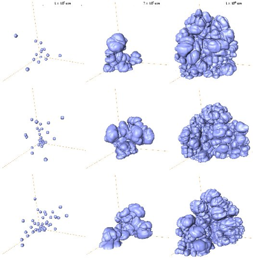
Figure 9: Evolution of the flame fronts in models b15_3d (top), b30_3d (middle), and b55_3d (bottom), at times $t=0\,\mathrm{s}$ (left column), $t=0.6\,\mathrm{s}$ (middle column), and $t=2.0\,\mathrm{s}$ (right column). The indicated length scale applies to the respective column.

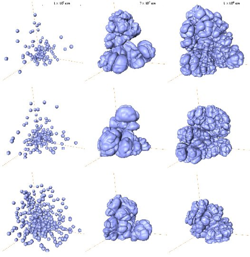
Figure 10: Evolution of the flame fronts in models b150_3d (top), b250_3d (middle), and b500_3d (bottom), at times $t=0\,\mathrm{s}$ (left column), $t=0.6\,\mathrm{s}$ (middle column), and $t=2.0\,\mathrm{s}$ (right column). The indicated length scale applies to the respective column.

The evolutions of the flame fronts in our three-dimensional models with multi-spot ignitions are shown in Figs. 9 and 10. As expected, the basic features are the same in all models and consistent with the findings of Reinecke et al. (2002b). After ignition in multiple spots, the volumes of the bubbles slowly increase due to the burning of the flame. In this first stage, buoyancy-induced flotation of the bubbles is slow since their dimension is small. Therefore the shear flows are weak and the effects of turbulent flame wrinkling increase only gradually. This corresponds to a slow increase of the released energies as can be seen from Fig. 8.

At $t\sim 0.4\,\mathrm{s}$ the energy generation rates increase drastically and peak around $0.6\,\mathrm{s}$. The flame fronts at this time are shown in the middle column of Figs. 9 and 10. We note here that the initially separated ignition spots have merged into a single connected structure in agreement with Reinecke et al. (2002b) and Röpke & Hillebrandt (2005a). As pointed out by Röpke & Hillebrandt (2005a) (see also Fig. 5 of that publication), this is a natural consequence of the flow field that establishes around buoyantly rising burning bubbles. The stream lines are directed around the forming mushroom-like structure and converge behind it, where an upwards pointing flow emerges. This flow drags underlying flame patches towards the bubble so that the originally disconnected flame structures eventually merge. This effect has been ignored in the dimensional estimate of Sect. 2.

After $t\sim 1.5\,\mathrm{s}$ the burning has ceased in our models and the energies released in the explosion process have reached their final values (cf. Fig. 8). The flame fronts at $t=2.0\,\mathrm{s}$ are shown in the right columns of Figs. 9 and 10. All models were followed up to $t=10.0\,\mathrm{s}$ where homologous expansion is reached with reasonable accuracy (Röpke, 2005). In the last seconds the distributions of the ashes change only slowly in the relaxation process.

From Figs. 9 and 10 it is obvious that the different ignition configurations lead to significant variations in the flame evolutions. They are determined by the effects mentioned in Sect. 2.

The first effect is most relevant in cases of small numbers of ignition spots. A sparse ignition may easily lead to anisotropies in the evolving flame structure. Due to the randomness of flame kernel locations the emerging large-scale flame structure is already imprinted in the ignition seed. This is most obvious in model b55_3d, where a preferential direction towards observer (cf. Fig.9, lower row) is already present in the ignition configuration and retained in the later evolution – although somewhat moderated in the latest stages. Since there are only very few ignition spots at large radii, i.e. subject to the large gravitational accelerations, these tend to produce the largest structures. This effect is, however, less pronounced than in the two-dimensional simulations. Thus, three-dimensional multi-spot models give rise to a more robust flame evolution.

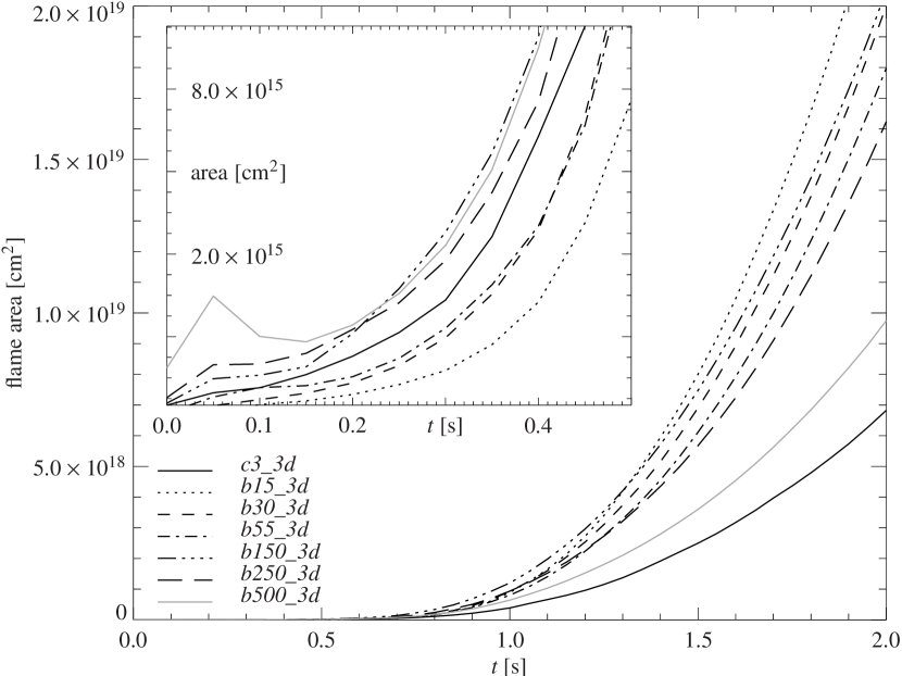
Figure 11: Flame surface area in different models as a function of time. The inset enlarges the evolution in the early stages.

As expected, with increasing number of ignition spots the flames will merge quickly due to burning and consequently flame surface is lost. To illustrate this effect, the temporal evolution of an approximate measure of the flame surfaces in the different models is plotted in Fig. 11. Obviously, they vary considerably. As a consequence of the dense distribution of initial flame bubbles in model b500_3d, the effect is most pronounced there. From ignition to $t=0.05\,\mathrm{s}$ the flame surface area increases rapidly, but it again decreases to a minimum between $t=0.1\,\mathrm{s}$ and $0.2\,\mathrm{s}$. The flame surface destruction effect is also present in a less pronounced way in the models b250_3d and b150_3d and even b55_3d. In these, the flame surfaces increase monotonically, but the slopes decrease between $t=0.05\,\mathrm{s}$ and $t=0.15\,\mathrm{s}$. In contrast, the surface destruction is not noticeable in simulations starting from sparse distributions of ignition spots. The slopes of flame surface area evolution increase monotonically in models b15_3d and b30_3d. Interestingly, the c3_3d model corresponds to an intermediate case.

The comparison of the later flame area evolution is more complicated. After $t\sim 1.0\,\mathrm{s}$ the flame surface areas of the models with sparse ignition seeds catch up with the models ignited in denser initial flame configurations. One possible explanation may be that in the latter, as soon as the initial flame seeds have merged due to burning, a new structure emerges which is similar to a single perturbed sphere. Since this large lump of ashes is generated in a random way, seeds for larger and perhaps dominating flame features may not emerge in a balanced distribution. Thus, the flame evolution may again be hampered by large scale modes as in the case of starting with sparse flame seeds and thus the loss in flame surface area may never be recovered.

It should be noted that the radius inside of which the flame kernels are ignited plays a minor role. In model b55_3d it was reduced by about 10% with little impact on the results.

6.3 Global quantities

The evolutions of the total energies in the models are plotted in Fig. 8. Values of the total energies, the nuclear energy releases, and the masses of produced iron group and intermediate mass nuclei and unburnt material at the end of our simulations ($t=10.0\,\mathrm{s}$) are included in Table 1. The masses of unburnt material in all models are too large to be consistent with observations. This is partially due to the fact that we stop burning artificially once the fuel density drops below $10^{7}\,\mathrm{g}\,\mathrm{cm}^{-3}$. Realistically, burning should continue to lower fuel densities converting more carbon/oxygen material into intermediate mass elements thereby increasing the energy release of the explosion (Röpke & Hillebrandt, 2005b).

The most vigorous explosion resulted from model b150_3d which released $1.18\times 10^{51}\,\mathrm{erg}$ of nuclear energy producing $0.667\,M_{\odot}$ of iron group elements and $0.167\,M_{\odot}$ of intermediate mass elements. The weakest explosion was obtained with the c3_3d initial flame configuration, but the model with most ignition spots, b500_3d, exploded almost as weakly. These global characteristics are a natural consequence of the flame area evolutions in the different models described above. The fact that model b15_3d finally develops the largest flame area is no contradiction. It catches up with the flame area of model b150_3d at $t\sim 1.3\,\mathrm{s}$, which is late in the burning phase of the simulation. At this time the burning is incomplete due to the low fuel densities in the expanded WD. It terminates in intermediate mass nuclei and the energy release is thus lower than in complete burning to nuclear statistical equilibrium (NSE) in earlier stages.

The global characteristics of the explosion models confirm the conjecture of Sect. 2. The explosion strength one can achieve with multiple ignition spots is indeed limited and there exists an optimal flame configuration with a finite number of initial flame kernels. Nevertheless, most multi-spot ignition scenarios show a significantly increased energy production as compared to the centrally ignited c3_3d simulation. It is remarkable that – in contrast to the two-dimensional models – most of the simulations reach total energies within a narrow range of about $0.7\times 10^{50}\,\mathrm{erg}$ around $6.3\times 10^{50}\,\mathrm{erg}$ (cf. Fig. 8 ). This may be interpreted as a sign for convergence and robustness of the multi-spot ignition model in its three-dimensional implementation. As far as the global quantities are concerned, even the most energetic explosion model b150_3d is not a clearly distinguished optimum, but all models starting with 15 to 250 ignition spots per octant reach similar explosion energies with some scatter due to the random choice of initial flame locations.

6.4 Distribution of elements in the ejecta

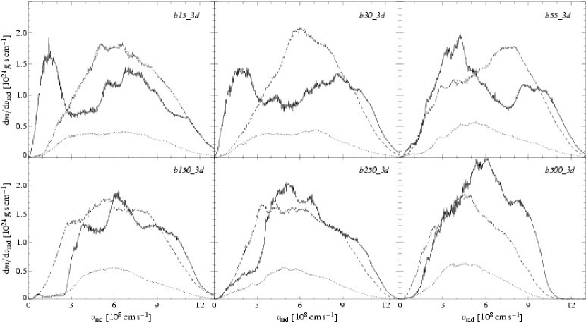
Figure 12: Distribution of the followed species in the three-dimensional models: carbon/oxygen fuel (solid) iron group elements (dashed), intermediate mass elements (dotted).

Besides the global quantities as the production of energy, other quantities can be compared with observational findings to judge the validity of SN Ia explosion models. These are mainly the abundances and distributions of various species in the explosion ejecta. Of course, most important is the radioactive isotope ⁵⁶Ni, since its decay powers the optical event, but also other isotopes contribute significantly to the shapes of spectra and light curves.

Constraints on abundances and distributions of elements can be obtained from comparing synthetic light curves and spectra derived from the models with observations. Alternatively, one can determine the composition stratification of the ejecta by fitting model spectra to a series of observed ones (Stehle et al., 2005) and compare it with the results of explosion models. Such detailed approaches are, however, beyond the scope of the present paper.

Without nuclear postprocessing (cf. Travaglio et al., 2004) we can only evaluate the cumulative abundances and distributions of iron group elements, intermediate mass elements, and unburnt material (carbon and oxygen). The produced masses of the former are given in Table 1. From comparison with the findings of Travaglio et al. (2004) it seems likely that the amounts of ⁵⁶Ni synthesized in the most strongly exploding models will be close to $0.4\,M_{\odot}$. This value falls within the range of the expectations for normal SNe Ia (Contardo et al., 2000), but rather on the low side.

The most interesting feature is the distribution of unburnt material in velocity space plotted in Fig. 12. Kozma et al. (2005) showed that spectra of the nebular phase put sharp constraints on the models in this respect. A synthetic nebular spectrum derived from a weakly exploding c3_3d model (but with a coarser flame resolution than the model presented here due to differences in the computational grids) featured strong emission lines originating from oxygen at low velocities. This effect might be an artifact of the peculiar (and unrealistic) c3_3d-configuration, where the large buoyant structures are already imprinted on the initial flame leading to strong downdrafts of unburnt material. It may be suspected that multi-spot ignition scenarios leading to different flame evolutions alleviate the downdraft problem. This could be possible due to the more complex initial flame structure which may be regarded as perturbed by a wider range of modes. Moreover, due to the large flame surface area that is achievable here, burning becomes more efficient and increased amounts of the sinking fuel in the downdrafts may be converted.

Indeed, this conjecture is supported by our results (cf. Fig. 12). In particular, in model b250_3d the unburnt material at low velocities is significantly reduced and the composition is dominated here by iron group elements. With increasing numbers of ignition spots a clear trend is noticeable from Fig. 12. Sparse distributions of initial flames still show an unburnt-material dominated composition at low velocities. With increasing numbers of ignition spots this gradually changes into an iron-group dominance. This effect is, however, not simply caused by the fact that with denser distributions of flame kernels more material is converted already in the ignition setup. The trend weakens with larger numbers of initial flames (cf. models b250_c3 and b500_c3 in Fig. 12). The reason is most likely again the effect of flame kernels melting together shortly after ignition, forming a large lump as described above. The emerging random perturbations of this structure are likely to prevent a balanced flame evolution similar to what is found in case of sparse ignition spot distributions. Such flame propagation scenarios naturally leave behind more unburnt material in central regions.

In contrast to the global quantities discussed in Sect. 6.3, the distribution of the species in the explosion ejecta clearly depends on the number of flame ignition kernels. Models with $\sim$150 ignition spots per octant produce distributions that are closest to observational expectations.

7 Conclusions

In the present study we have explored the possibilities of multi-spot ignition scenarios of Type Ia supernova explosion models in a systematic way. Owing to improvements of the computational code, it was possible to achieve a high initial resolution of $1.74\,\mathrm{km}$ on computational grids with 256 cells per dimension. By setting the initial bubble radii to $5.5\,\mathrm{km}$, it was possible to accommodate up to 500 flame kernels within a radius of $\sim$$180\,\mathrm{km}$ around the center of the WD star. Due to the random placement and overlap of the bubbles, larger structures emerge providing a variety of sizes of ignition seeds.

Comparing the results of two-dimensional simulations with those of three-dimensional models, we find significant differences in the flame front evolutions starting from multiple ignition spots. In the former setups, single outliers tend to dominate the evolution to a much higher degree than in three dimensions. We conclude from these findings that two-dimensional simulations are inappropriate to explore initial flame configurations. Two-dimensional studies can therefore only be a tool to study other effects and compare simulations with the same fixed and carefully chosen initial flame configuration, a possibility being the c3_2d-model. Thus, although the general picture of our two-dimensional simulations is similar to the findings of Livne et al. (2005), we disagree with their conclusions.

A simple estimate showed that the gain in explosion strength arising from multi-spot ignition scenarios should be limited. This is confirmed by a systematic study based on three-dimensional simulations covering one octant of the star. Different ignition configurations with 15 up to 500 flame seeds were tested. We found the most vigorously exploding model for 150 flame kernels per octant with a radial Gaussian distribution inside a sphere of $180\,\mathrm{km}$ around the center of the WD. This agrees reasonably with our dimensional estimate in Sect. 2, given the simplifications made there. Setups with increased resolutions – although allowing for smaller flame seeds – would not profit from much higher numbers of ignition spots.

In terms of production of energy and iron group elements this simulation came close to the b30-model of Travaglio et al. (2004), which is a success of the hybrid grid implementation since it allows results on an only $[256]^{3}$ cells computational grid that previously required $[768]^{3}$ cells. This novel approach will provide a powerful tool to study the details of SN Ia deflagration models at moderate computational expenses. The similarity with the b30-model suggests that the deflagration scenario of SNe Ia in its current implementation (i.e. applying a multi-spot ignition with a Gaussian radial distribution within $\sim$$180\,\mathrm{km}$ around the center of the WD and ignoring burning below fuel densities of $10^{7}\,\mathrm{g}\,\mathrm{cm}^{-3}$) will not allow asymptotic kinetic energies much higher than $\sim$$7\times 10^{50}\,\mathrm{erg}$ and the total production of iron group elements will not greatly exceed $0.7\,M_{\odot}$. Since these values already fall in the range of observational expectations (cf. eg. Contardo et al., 2000), multi-spot ignition scenarios offer a way of modeling “normal” SNe Ia events. These global quantities seem to be rather robust against variations in the number and configuration of flame kernels.

Comparing our results with those of García-Senz & Bravo (2005) we note agreement in some general results. Multi-spot ignition scenarios may give rise to an explosion of the WD star. The evolution of the large-scale features is similar in both studies. Our novel approach, however, facilitated an increased resolution of the initial flame configuration by a factor of 10 compared with García-Senz & Bravo (2005). It was therefore possible to accommodate much smaller flame kernels in greater numbers within the ignition region. This may be the main reason for disagreements in the conclusions (our more elaborate flame description certainly contributes as well, but this is difficult to disentangle). In contrast to García-Senz & Bravo (2005) our results do not indicate a convergence with ever increasing numbers of flame seeds, but rather a maximum at a limited number. Moreover, our initial flame bubbles seem to merge more rapidly forming a connected flame structure. This gives rise to differences in the distribution of species in the ejecta. The clumpiness of ashes reported by García-Senz & Bravo (2005) is less pronounced in our simulations.

In cases with larger numbers of ignition spots, we find a much better exhaustion of the fuel in central regions. In contrast to the global quantities, this effect is sensitive to the number of ignition spots, indicating an incompleteness of the current deflagration model of SNe Ia. Potentially, an improved modeling of late phases of the burning process (Röpke & Hillebrandt, 2005b) may be necessary, which possibly also increases the explosion energy.

We conclude from our simulations that multi-spot ignition scenarios may allow SN Ia models to achieve better agreement with observations, although the effect is limited with regard to the number of igniting flames. It thus does not lead to an arbitrary means of tuning the models to higher energy release or nuclear conversion in the explosive burning. Multi-spot ignition scenarios, however, may be capable of reproducing “normal” SN Ia explosions.