Constraining Inverse Curvature Gravity with Supernovae

Abstract

We show that the current accelerated expansion of the Universe can be explained without resorting to dark energy. Models of generalized modified gravity, with inverse powers of the curvature can have late time accelerating attractors without conflicting with solar system experiments. We have solved the Friedman equations for the full dynamical range of the evolution of the Universe. This allows us to perform a detailed analysis of Supernovae data in the context of such models that results in an excellent fit. Hence, inverse curvature gravity models represent an example of phenomenologically viable models in which the current acceleration of the Universe is driven by curvature instead of dark energy. If we further include constraints on the current expansion rate of the Universe from the Hubble Space Telescope and on the age of the Universe from globular clusters, we obtain that the matter content of the Universe is $0.07\leq\omega_{\rm m}\leq 0.21$ (95% Confidence). Hence the inverse curvature gravity models considered can not explain the dynamics of the Universe just with a baryonic matter component.

PACS:04.50.+h, 95.36.+x

It is now widely accepted that recent Supernovae (SNe) observations imply that our Universe is currently experiencing a phase of accelerated expansion Riess:1998cb . This seems to be independently confirmed by observations of clusters of galaxies Allen:04 and the cosmic microwave background WMAP . The accelerated expansion is usually explained through violations of the strong energy condition by introducing an extra component in the Einstein equations in the form of dark energy with an equation of state $w<-1/3$. However, such an explanation is plagued with theoretical and phenomenological problems, such as the extreme fine tuning of initial conditions and the so called coincidence problem Steinhardt and it is therefore natural to seek alternatives to dark energy as the source of the acceleration. One possibility is an inhomogeneous Universe with only local acceleration, albeit it is hard to explain natural boundary conditions for such a local void Kolb:2005me . The other, that we will elaborate on in this Letter, is modifications of gravity that turn on only at very large distances Gabadadze:2004dq or small curvatures Carroll:2003wy ; Capozziello:2003tk therefore giving a geometrical origin to the accelerated expansion of the Universe.

It was shown in Carroll:2003wy that a simple modification of the gravitational action adding inverse of curvature invariants to the Einstein-Hilbert term would naturally have effects only at low curvatures and therefore at late cosmological times. The simplest of such modifications includes just one single inverse of the curvature scalar $\mu^{4}/R$, with $\mu$ a parameter with dimensions of mass. This results in a model governed by the Einstein-Hilbert term, i.e. usual gravity, for curvatures $R\gg\mu^{2}$ but can lead to an accelerated expansion at curvatures $R\lesssim\mu^{2}$. This simple model is equivalent to a Brans-Dicke theory Carroll:2003wy . Based on this equivalence it was subsequently proven by a number of authors that the model is in conflict with solar system data solarsystem and is unstable when matter is introduced Dolgov:2003px . This conclusion naturally extends to generalizations of this action where the Einstein-Hilbert term is supplemented with an arbitrary function of $R$, except for particular cases that could still lead to viable models Dick:2003dw .

With this restriction in mind, the authors of Carroll:2004de discussed a more general modification of gravity based on the following gravitational action

$$\begin{array}[]{lcl}\displaystyle S&\displaystyle=&\displaystyle\frac{1}{16\pi G}\int d^{4}x\sqrt{-g}\Big{[}R-\frac{\mu^{4n+2}}{(aR^{2}+bP+cQ)^{n}}\Big{]}\\ &\displaystyle+&\displaystyle\int d^{4}x\sqrt{-g}\mathcal{L}_{M}\;,\end{array}$$ (1)

where $P\equiv R_{\mu\nu}R^{\mu\nu}$, $Q\equiv R_{\mu\nu\rho\sigma}R^{\mu\nu\rho\sigma}$, $G$ Newton’s constant, ${\cal L}_{M}$ the matter Lagrangian and $g$ the determinant of the metric.

In this generalized case the equivalence with a Brans-Dicke theory is not clear and a more detailed analysis of modifications of Newton’s potential has to be done to compare with solar system data. The authors of Navarro:2005gh computed the corrections to Newton’s law in these models as a perturbation around Schwarzschild geometry and found that as long as we include inverse powers of the Riemann tensor ($c\neq 0$), Newton’s law is not modified in the solar system at distances shorter than $r_{c}\sim 10$ pc and therefore all solar system experiments are well under control. Note that, as long as the Riemann tensor is present, this result is independent of whether we include or not inverse powers of the scalar curvature or the Ricci tensor squared, as they vanish in the background solution. This important result restricts the parameter space of phenomenologically relevant inverse curvature gravity models to the ones with inverse powers of the Riemann tensor squared present. Other constraints come from the absence of ghosts in the spectrum, requiring specific relations between $b$ and $c$ Navarro:toappear . Finally we restrict our analysis in this Letter to models with $n=1$.

Let us turn now to the cosmology of models governed by the gravitational action (1). Assuming a cosmological setup with a spatially flat Friedmann-Robertson-Walker metric, $ds^{2}=-dt^{2}+a(t)d\vec{x}^{2}$, all models with $n=1$ can be characterized by just three parameters, $\alpha$, $\hat{\mu}$ and $\sigma$, given in terms of the parameters in Eq. (1) by

$$\alpha\equiv \frac{12a+4b+4c}{12a+3b+2c},$$ (2)

$$\hat{\mu}\equiv \mu/|12a+3b+2c|^{1/6},$$ (3)

$$\sigma\equiv \mathrm{sign}(12a+3b+2c).$$ (4)

In order to write the corresponding Friedmann equation in the simplest possible way we will use logarithmic variables, $u\equiv\ln(H/\hat{\mu})$ and $N\equiv\ln a$, where as usual $H=\frac{\dot{a}}{a}$, with a dot denoting the time derivative. The generalized Friedmann equation in these variables reads

$$u^{\prime\prime}\mathcal{P}_{1}(u^{\prime})+\mathcal{P}_{2}(u^{\prime})+18\sigma\big{(}\mathcal{P}_{3}(u^{\prime}))^{3}e^{6u}(e^{2(\bar{u}-u)}-1)=0,$$ (5)

where a prime denotes the derivative with respect to $N$ and we have defined the following polynomials,

$$\mathcal{P}_{1}(y) =6\alpha^{2}y^{2}+24\alpha y+32-8\alpha,$$ (6)

$$\mathcal{P}_{2}(y) =15\alpha^{2}y^{4}+2\alpha(50-3\alpha)y^{3}$$

$$+4(40+11\alpha)y^{2}+24(8-\alpha)y+32,$$ (7)

$$\mathcal{P}_{3}(y) =\alpha y^{2}+4y+4\;.$$ (8)

The source is $\bar{u}\equiv\ln\left[\bar{\omega}_{r}\exp(-4N)+\bar{\omega}_{m}\exp(-3N)\right]/2$, where we have defined the appropriately normalized values of the energy densities today as

$$\frac{8\pi G}{3}\frac{\rho_{r,m\,0}}{\hat{\mu}^{2}}\equiv\bar{\omega}_{r,m}\;,$$ (9)

with $\rho_{\rm r,m}^{0}$ the present densities in matter and radiation and we have exploited the fact that the energy-momentum tensor is still covariantly conserved. This means that the source in Eq. (5) corresponds to the standard one with no dark energy.

The new Friedmann equation is no longer algebraic but a second order non-linear differential equation. Furthermore, it becomes non-autonomous in the presence of sources, making its dynamical study a formidable problem. The asymptotic behavior of the system in vacuum was carefully studied in Carroll:2004de , where it was found that, depending on the value of $\alpha$, but irrespective of $\sigma$, the system has a number of attractors, including sometimes singularities. The same attractor and singular points are relevant when sources are present. In that case however, both the value of $\sigma$ and the fact that the Universe is in a matter dominated era before the new corrections become relevant are crucial to determine the fate of the Universe.

A careful analysis of the dynamical behavior of the system reveals that physically valid solutions only exist for certain combinations of $\alpha$ and $\sigma$. In order to classify the different regions, we define the following special values of $\alpha$: $\alpha_{1}\equiv 8/9$, $\alpha_{2}\equiv 4(11-\sqrt{13})/27\approx 1.095$ and $\alpha_{3}\equiv 20(2-\sqrt{3})/3\approx 1.786$. For $\alpha<\alpha_{1}$ both signs of $\sigma$ result in an acceptable (non-singular) dynamical evolution, but nevertheless in a bad fit to Supernovae data. For $\alpha_{1}<\alpha<\alpha_{2}$ only $\sigma=-1$ leads to an acceptable expansion history, since for $\sigma=+1$ a singular point is violently approached in the past. For $\alpha_{2}<\alpha$ the singular point is approached for $\sigma=-1$, hence $\sigma=+1$ is the only physically valid solution. In this latter case, when $\alpha_{2}<\alpha<\alpha_{3}$, the system goes to a stable attractor that is decelerated, thus giving a bad fit to SNe data, for $\alpha<32/21$ and gets accelerated for larger $\alpha$. For $\alpha_{3}<\alpha$ there is no longer a stable attractor and the system smoothly goes to a singularity in the future. That singularity occurs earlier as $\alpha$ increases so that there is a limiting function $\alpha_{4}(\bar{\omega}_{m})$, at which the singularity is reached today. It is important to stress that this singularity is approached in a very smooth fashion, allowing for a phenomenologically viable behavior of the system, as opposed to the evolution when the wrong value of $\sigma$ is chosen, where the singularity is hit almost instantaneously. Finally, for values of $\alpha\gtrsim 24.9$, there are stable attractors again but these are never accelerated and the resulting fit to SNe data is not acceptable. To summarize, there are two regions that give a dynamical evolution of the system compatible with SNe data, the low region with $\alpha_{1}<\alpha<\alpha_{2}$, for which $\sigma=-1$, and the high region where $\alpha_{2}<\alpha<\alpha_{4}$, for which $\sigma=+1$.

As we have emphasized it is extremely difficult to solve the dynamics of the system analytically. To overcome this limitation we have performed a comprehensive numerical study of the model resulting in the general behavior we have outlined above. To make things more complicated the new Friedmann equation is extremely stiff, due to the exponentials in the last term. This stiffness is directly linked to the nature of the corrections that are negligibly small in the far past, where the curvature is much smaller than the scale $\hat{\mu}^{2}$. It also makes it essentially impossible to numerically integrate it from a radiation dominated era all the way to the present. In order to circumvent this problem, we have matched a perturbative analytical solution that tracks the solution in standard Einstein gravity in the far past to the corresponding numerical one in the region $z\gtrsim 5$, where the analytical solution is still an extremely good approximation, and the numerical codes can cope with the integration. Although the matching at this point is accurate below the 1% level, we emphasize that it is safely above the redshift range probed by SNe. The approximate solution from the perturbation analysis, for $\alpha\neq 8/9$, is given by

$$H_{\mathrm{approx}}=\hat{\mu}e^{\bar{u}}\left(1+\frac{e^{-6\bar{u}}}{36\sigma}\frac{\bar{u}^{\prime\prime}\mathcal{P}_{1}(\bar{u}^{\prime})+\mathcal{P}_{2}(\bar{u}^{\prime})}{\big{(}\mathcal{P}_{3}(\bar{u}^{\prime})\big{)}^{3}}\right).$$ (10)

This is an extremely accurate solution to the full non-linear equation as long as $z\gtrsim 5$, regardless of the values of $\alpha$ and ${\bar{\omega}}_{m}$. At the boundaries between regions with different dynamical behavior (including $\alpha_{1}$) the sensitivity to initial conditions is large and therefore nothing conclusive can be said at these points. The question of sensitivity to initial conditions is a relevant one due to the non-linear nature of Friedmann equation. However due to the complication of any analytical study for non-negligible sources alluded to above we will defer its study to a future publication. In the present Letter we will contempt ourselves with the particular solution in Eq. (10) that we are guaranteed tracks the standard behavior in Einstein gravity in the past. We further explicitly confirmed, by a numerical analysis, that our conclusions are not sensitive to the exact position of the matching point in the past.

Once we have solved for the Hubble parameter as a function of the scale factor, we perform a fit to SNe data to get the allowed values of the different parameters defining our model. In principle there is a total of five parameters defining our Universe in this framework, namely the three parameters defining the model, $\hat{\mu}$, $\alpha$ and $\sigma$, and the two parameters determining the sources, $\bar{\omega}_{r,m}$. The absolute value of the CMB temperature, however, fixes the total radiation content of the Universe, constraining $\bar{\omega}_{r}\hat{\mu}^{2}$. For relevant values of $\hat{\mu}$ this constraint makes radiation irrelevant in the analysis of SNe data. Since the intrinsic magnitude of SNe is a nuisance parameter in our analysis, it is not possible to determine $\hat{\mu}$ as an independent parameter with SNe only. For a standard $\Lambda$CDM Universe this corresponds to the inability of SNe data to independently determine the Hubble constant $H_{0}$. However, we will be able to determine the value of $\hat{\mu}$ once we impose other constraints, like the measurement of the Hubble constant by the Hubble Key Project, $H_{0}=72\pm 8$ Km s^-1 Mpc^-1 Freedman:2000cf . Hence, this leaves us with just three parameters, $\alpha$, $\sigma$ and $\bar{\omega}_{m}$ relevant for the analysis of SNe data and an additional nuisance parameter in terms of the intrinsic magnitude.

The fits are performed using the recent gold SNe data set from the last reference in Riess:1998cb . The apparent magnitude is given by $m(z)=\mathcal{M}+5\log\mathcal{D}_{L}$ where $\mathcal{M}\equiv M-5\log\hat{\mu}+25$ and $\mathcal{D}_{L}\equiv\hat{\mu}d_{L}$ with $d_{L}\propto\int H^{-1}(z)dz$. Note that the parameter $\hat{\mu}$ appears in the definition of the magnitude compared to the usual definition involving $H_{0}$ Riess:1998cb . The important point is that $\mathcal{D}_{L}(z)$ can now be computed solely in terms of $\bar{\omega}_{m}$ and $\alpha$, where $\hat{\mu}$ and the intrinsic magnitude have been absorbed into the nuisance parameter $\mathcal{M}$ that can be marginalized analytically in the probability function.

We have performed independent two parameter fits to SNe data for each of the low and high regions. This results in the 1- and 2-$\sigma$ joint likelihoods shown in Fig.1,

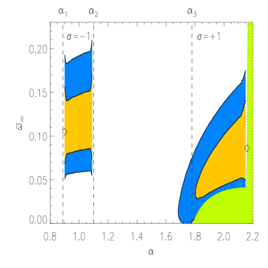
Figure 1: 1 and 2-$\sigma$ joint likelihoods on ${\bar{\omega}}_{m}$ and $\alpha$. In the low region $\sigma=-1$ whereas in the high region $\sigma=+1$. The shaded area on the right determines the region $\alpha>\alpha_{4}$ that is excluded because of a singularity being hit in the past. The diamonds denote the maximum likelihood points.

with best fit values given by

$$\mathit{low}:\,\alpha=0.9,\quad\bar{\omega}_{m}=0.105,\quad\chi^{2}=184.9,$$ (11)

$$\mathit{high}:\alpha=2.15,\quad\bar{\omega}_{m}=0.085,\quad\chi^{2}=185.2.$$ (12)

For comparison purposes, we have also performed the fit using the standard $\Lambda CDM$ model for a spatially flat Universe and absorbing $H_{0}$ as a nuisance parameter into ${\cal M}$, resulting in $\chi^{2}=184.9$ for $156$ data points. We further show in Fig. 1 the points $\alpha_{i}$. The shaded area on the right side, which is bordered by a dotted line, is the exclusion zone given by $\alpha_{4}(\bar{\omega}_{\rm m})$. Note that the contours have a sharp cut-off at $\alpha_{1}$, $\alpha_{2}$ and $\alpha_{4}$. However at $\alpha_{3}$ there is no singularity hit violently and the $2-\sigma$ contour of the high region extends below $\alpha_{3}$. In the low region we obtain $\bar{\omega}_{\rm m}=0.122\pm 0.034$ after marginalization over $\alpha$ and in the high region $\bar{\omega}_{\rm m}=0.075\pm 0.031$. Note that our best fit points in both regions are close to the borders of the allowed region. This is because within the regions there is a smooth behavior of the likelihood, and only the dynamics of the system cuts off the likelihood space if certain parameter values are reached.

If we additionally apply the HST measurement of $H_{0}$, Freedman:2000cf we can determine $\hat{\mu}$ and the matter content $\omega_{\rm m}=\Omega_{\rm m}h^{2}$, with $H_{0}=100h\,{\rm km/s/Mpc}$. Finally we can restrict the allowed region in $\omega_{\rm m}-\hat{\mu}$ a little bit more by imposing a prior on the age of the Universe with a mean of $t_{0}=13.4$ Gyrs and a 95% confidence lower limit of $11.2$ Gyrs Krauss:03 .

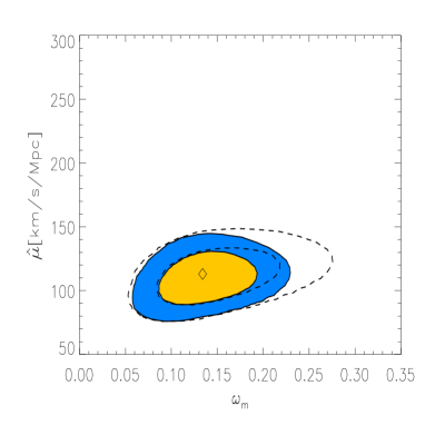
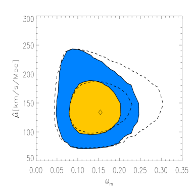
Figure 2: The 1- and 2-$\sigma$ joint likelihoods in the $\omega_{\rm m}-\hat{\mu}$ plane, when additional priors on $H_{0}$ and the age of the Universe are imposed. On the left for the low region and on the right for the high region. Diamonds are the maximum likelihoods. Further, the dashed contours are the joint likelihoods if we impose only the $H_{0}$ prior.

In Fig. 2 we show the joint 1- and 2-$\sigma$ likelihoods in the $\omega_{m}$-$\hat{\mu}$ plane, with both priors imposed (solid line) and without imposing the age of the Universe prior (dashed line). On the left for the low region and on the right for the high region. First we recognize that $\hat{\mu}$ is roughly twice the size of the Hubble constant $H_{0}$. If we further marginalize over $\hat{\mu}$ the physical matter content in the Universe is $\omega_{\rm m}=0.14\pm 0.03$ and $\omega_{\rm m}=0.14\pm 0.04$ in the low and high regions, respectively. Note that the matter content in the budget of the Universe is clearly higher than the measured baryonic content. Overall we find $0.07\leq\omega_{\rm m}\leq 0.21$ at the 95% confidence level. If we compare this number with the results from Big Bang Nucleosynthesis $\omega_{\rm b}=0.0214\pm 0.0020$ Kirkman:03 it is clear that we require a dark matter component to explain the data.

Other cosmological probes such as clusters of galaxies and CMB could further constrain these models. However such an analysis is beyond the scope of this Letter since it requires a detailed re-calculation of, e.g. cluster potentials and CMB perturbations for the models discussed here.

Summary: We have studied the viability of a geometrical explanation for the present acceleration of the Universe. This is possible if the Einstein-Hilbert action is supplemented with new terms that are negligibly small at high cosmological curvatures but become relevant when the curvature of the Universe gets smaller. Despite the phenomenological problems of the simplest models, it has been shown that there exists a broad class of modifications of gravity that are phenomenologically viable and have accelerated attractors at late-times. In this Letter we have performed a detailed numerical analysis of the dynamics of these models. We emphasize that this hard numerical problem has not been solved previously. The result of this analysis allowed us to compare inverse curvature gravity with Supernovae data. We found that SNe data can be fitted in our model without the need of any dark energy and getting meaningful constraints in the free parameters. We further have shown that these models still require a dark matter component. Of course this latter conclusion does not need to hold for more general models, for instance those with $n\neq 1$. We are planning to study more general models and their implications for dark matter in the near future. However, we would like to emphasize the generality of our study. We have parameterized all models governed by Eq. (1) with $n=1$. Finally we are currently extending this analysis to CMB and cluster datasets, a non-trivial task. This will further constrain these models and maybe even distinguish them from dark energy.

Acknowledgments: It is a pleasure to thank R. Battye, G. Bertone, S. Dodelson, A. Lewis, M. Liguori, I.Navarro for useful conversations. This work is supported by DOE and NASA grant NAG 5-10842.

References

- (1) A. G. Riess et al. [Supernova Search Team Collaboration], Astron. J. 116 (1998) 1009 [arXiv:astro-ph/9805201]; S. Perlmutter et al. [Supernova Cosmology Project Collaboration], Astrophys. J. 517 (1999) 565 [arXiv:astro-ph/9812133]; N. A. Bahcall, J. P. Ostriker, S. Perlmutter and P. J. Steinhardt, Science 284 (1999) 1481 [arXiv:astro-ph/9906463]; A. G. Riess et al. [Supernova Search Team Collaboration], Astrophys. J. 607 (2004) 665 [arXiv:astro-ph/0402512].
- (2) S. W. Allen, R. W. Schmidt, H. Ebeling, A. C. Fabian and L. van Speybroeck, Mon. Not. Roy. Astron. Soc. 353 (2004) 457 [arXiv:astro-ph/0405340]; D. Rapetti, S. W. Allen and J. Weller, Mon. Not. Roy. Astron. Soc. 360 (2005) 555 [arXiv:astro-ph/0409574].
- (3) D. N. Spergel et al. [WMAP Collaboration], Astrophys. J. Suppl. 148 (2003) 175 [arXiv:astro-ph/0302209].
- (4) I. Zlatev, L. M. Wang and P. J. Steinhardt, Phys. Rev. Lett. 82 (1999) 896 [arXiv:astro-ph/9807002].
- (5) E. W. Kolb, S. Matarrese, A. Notari and A. Riotto, arXiv:hep-th/0503117; E. W. Kolb, S. Matarrese and A. Riotto, arXiv:astro-ph/0506534.
- (6) G. Gabadadze, arXiv:hep-th/0408118.
- (7) S. M. Carroll, V. Duvvuri, M. Trodden and M. S. Turner, Phys. Rev. D 70 (2004) 043528 [arXiv:astro-ph/0306438].
- (8) S. Capozziello, S. Carloni and A. Troisi, arXiv:astro-ph/0303041; D. N. Vollick, Phys. Rev. D 68 (2003) 063510 [arXiv:astro-ph/0306630].
- (9) T. Chiba, Phys. Lett. B 575 (2003) 1 [arXiv:astro-ph/0307338]; M. E. Soussa and R. P. Woodard, Gen. Rel. Grav. 36 (2004) 855 [arXiv:astro-ph/0308114]; G. J. Olmo, Phys. Rev. D 72 (2005) 083505.
- (10) A. D. Dolgov and M. Kawasaki, Phys. Lett. B 573 (2003) 1 [arXiv:astro-ph/0307285].
- (11) R. Dick, Gen. Rel. Grav. 36 (2004) 217 [arXiv:gr-qc/0307052]; S. Nojiri and S. D. Odintsov, Phys. Rev. D 68 (2003) 123512 [arXiv:hep-th/0307288]; Gen. Rel. Grav. 36 (2004) 1765 [arXiv:hep-th/0308176].
- (12) S. M. Carroll, A. De Felice, V. Duvvuri, D. A. Easson, M. Trodden and M. S. Turner, Phys. Rev. D 71 (2005) 063513 [arXiv:astro-ph/0410031].
- (13) I. Navarro and K. Van Acoleyen, Phys. Lett. B 622 (2005) 1 [arXiv:gr-qc/0506096].
- (14) I. Navarro and K. Van Acoleyen, to appear.
- (15) W. L. Freedman et al., Astrophys. J. 553 (2001) 47 [arXiv:astro-ph/0012376].
- (16) L. M. Krauss and B. Chaboyer, Science, 299 (2003) 65.
- (17) D. Kirkman, D. Tytler, N. Suzuki, J. M. O’Meara and D. Lubin, Astrophys. J. Suppl. 149 (2003) 1 [arXiv:astro-ph/0302006].