Lightcurves of 20–100 kilometer Kuiper Belt Objects using the Hubble Space Telescope

Abstract

We report high precision photometry of three small and one larger Kuiper Belt Objects (KBOs) obtained with the Advanced Camera for Surveys onboard the Hubble Space Telescope (ACS/HST). The three small bodies are the smallest KBOs for which lightcurve measurements are available. 2003 BF₉₁ has a diameter of 20 kilometers (assuming 10% albedo) and a 1.09 magnitude, 9.1-hour lightcurve that is feasibly explained by the rotation of an elongated, coherent body that is supported by material strength and best imagined as an icy outer Solar System analog to asteroid (243) Ida. Two other small KBOs, 2003 BG₉₁ and 2003 BH₉₁ (diameters 31 and 18 km, with albedo 10%), exhibit an unremarkable lightcurve and no detectable photometric variation, respectively. For the larger KBO 2000 FV₅₃ (116 km diameter, assuming 10% albedo) we strongly detect a non-sinusoidal periodic (7.5 hours) brightness variation with a very small amplitude (0.07 mag). This KBO may be nearly spherical, a result that might not be unusual in the Kuiper Belt but would be remarkable among outer Solar System satellites of similar size.

Lightcurves may be caused by variations in albedo or shape, and we carry out a study of possible physical states and bulk densities under the assumptions of both fluid equilibrium and finite, non-zero internal friction. Under most assumptions, the densities for the these KBOs are likely to be in the range 1–2 g cm^-3, and a plausible solution for 2000 FV₅₃ is a rubble pile of this density that is held slightly out of the minimum-energy shape by internal friction among constituent blocks that are relatively small. Our interpretation of 2000 FV₅₃ as a pulverized but essentially primordial object and 2003 BF₉₁ as a collisional fragment is consistent with models of collisional timescales in the outer Solar System. We compile all published KBO lightcurve data to date and compare our results to the larger population.

1 Introduction

The Kuiper Belt, a remnant debris disk that surrounds the planetary realm of our Solar System, is a relatively pristine record of the prevailing conditions during the formation of the Solar System. Subsequent evolution has overprinted this original state such that present day observations allude to the combination of accretion and eons of collisions. Observations of individual Kuiper Belt Objects (KBOs) allow explorations of bodies with aged, but primordial, compositions. Studies of binary KBOs (Veillet et al., 2002; Noll et al., 2002; Osip et al., 2003; Noll et al., 2004a, b; Stansberry et al., 2005; Stephens & Noll, 2005) provide albedo constraints, usually under a density assumption, and may increase what little is known about the internal composition and structure of KBOs.

Small Solar System body lightcurves have been studied for many years, principally for asteroids (Pravec et al., 2002) and comets (see, e.g., Jewitt (1991); Samarasinha et al. (2004)). Lightcurves of small objects are often interpreted as manifestations of reflections from irregularly shaped objects, and lightcurve information has been shown to correspond well with radar-derived shape models (see, e.g., Ostro et al. (2002)). With the continued increase in the number of known KBOs (and hence bright KBOs) and access to improving observing technologies, KBO lightcurves can now be studied. Published lightcurve data exist for 65 KBOs and Centaurs, with approximately half showing lightcurves greater than around 0.1 magnitudes with a typical amplitude around 0.5 magnitudes. 2001 QG₂₉₈ has the largest known KBO lightcurve amplitude of 1.14 magnitudes (Sheppard & Jewitt, 2004). KBO lightcurves are though to imply either heterogeneous albedo distributions or else asphericities, with the extreme case of the latter potentially being contact binary KBOs (Sheppard & Jewitt, 2004). The KBO lightcurve literature is tabulated and analyzed in Section 6.3.

Here we report high precision photometry for four KBOs observed with the Hubble Space Telescope (Section 2). The capabilities of the HST and the extended duration of this study permit, for the first time, the study of photometric variations of very faint and therefore small KBOs and the detection of very small ($<0.1$ mag) variations of modest-sized KBOs. Two of these KBOs show clear periodic variation; a third shows a somewhat less significant periodic variation; and the fourth has no distinguishable periodic signature (Section 3). We discuss interpretations of this data in Sections 4 and 5 and the implications in Section 6.

2 Observations

We have carried out a large (125 orbits) Hubble Space Telescope/Advanced Camera for Surveys (HST/ACS) observing program to search for very faint KBOs. The primary results of this program — discovery of a substantial deficit of classical and excited KBOs at small sizes — are reported in Bernstein et al. (2004). Here we briefly summarize the relevant technical details of the observations and data reduction (see Bernstein et al. (2004) for complete discussions). Our observations were divided into two epochs, the “discovery epoch” (UT 2003 January 26.014–31.341), in which $55\times 400$ s exposures were taken at each of the six pointings; and the “recovery epoch” (2003 February 05.835–09.703), in which an additional $40\times 400$ s exposures were taken at each pointing. During the discovery epoch, a given pointing is sampled sporadically, with intervals as small as 8 minutes, over a time span of approximately 24 hours; the pointing is revisited 2 days later with the same sporadic sampling. Approximately 7 days later, the entire cycle repeats for the recovery epoch. Consequently, we obtained $\approx 95$ independent measurements of each KBO observed, over a time baseline of around 12 days, with sampling as fine as minutes in some cases but with windows of several days (or more) in which no observations of a given KBO were made.

Bernstein et al. (2004) detected three new KBOs (2003 BF₉₁, 2003 BG₉₁, and 2003 BH₉₁) as well as a previously known KBO (2000 FV₅₃) that was targeted in the observations. 2000 FV₅₃ was detected with signal-to-noise ratio $S/N\geq 80$ in each of its individual exposures; hence, the photometry is quite precise. 2003 BG₉₁, 2003 BF₉₁, and 2003 BH₉₁ were discovered with $S/N$ in individual exposures typically 7.5, 2.7, and 2.4, respectively. Discovery of the last object required the use of “digital tracking,” in which exposures are shifted at rates corresponding to all valid KBO orbits before summing and searching for flux peaks that exceed the detection threshold.

Photometry for each object was extracted by fitting a model of a moving point source to relevant exposures. We measured the point spread function (PSF) for the ACS Wide Field Camera (WFC) in exposures of a globular cluster field. In the moving point source model-fitting, this PSF was smeared before fitting to the relevant pixels to account for the (slight) trailing expected on each exposure. We fit the entire stack of images simultaneously, with the free parameters being the 6 relevant degrees of freedom in the KBO orbit plus an unknown flux for each exposure. The best-fit photometry and orbit are thus solved simultaneously.

The $S/N$ per exposure for 2000 FV₅₃ is so high that we use a slightly different approach, allowing the position to be a free parameter on each exposure rather than forcing positions to obey a common orbit. Without this approach, we find that small (milliarcsecond) errors in the astrometric solutions for the WFC cause excess variance in the flux determinations. For the fainter three KBOs, the flux errors due to these $\sim$5 milliarcsecond astrometric errors are a few hundredths of a magnitude, well below the noise levels. The slow brightening due to the decreasing illumination phase of the KBOs is too small to be detected in our data.

The fitting process produces uncertainties for each flux measurement. We find that the best-fit sinusoidal light curves give $\chi^{2}$ per degree of freedom (DOF) near unity for the three faint bodies (see below), suggesting that our error estimates are reliable. The $\chi^{2}$ for the best sinusoidal fit for 2000 FV₅₃ is too high, partly because the light curve is clearly not sinusoidal (see below), but also because various systematic effects (e.g., pointing jitter) may affect the PSF fitting at the 0.01 mag level. The formal errors on the magnitudes may also be underestimated, as is common for very high $S/N$ photometry.

The midpoint time of each exposure is corrected for light-travel time from the target. The time-series photometry for these four objects is presented in Tables 1 – 4.

Table 1: Photometry for 2003 BG₉₁

MJD	Flux (electrons/sec)
52666.1767	0.3777 $\pm$ 1.8490
52666.1803	0.8904 $\pm$ 0.1151
52666.1860	0.8166 $\pm$ 0.1134
52666.1918	0.7036 $\pm$ 0.1110
52666.1975	0.8721 $\pm$ 0.1173
52666.2033	0.8127 $\pm$ 0.1168
52666.2421	0.6223 $\pm$ 0.0983
52666.2487	0.8509 $\pm$ 0.1043
52666.2552	0.9279 $\pm$ 0.1058
52666.2618	0.8789 $\pm$ 0.1041
52666.2683	0.7230 $\pm$ 0.1056
52666.3089	0.5674 $\pm$ 0.0968
52666.3154	0.8129 $\pm$ 0.1035
52666.3220	0.8537 $\pm$ 0.1002
52666.3285	0.6708 $\pm$ 0.0992
52666.3351	1.0203 $\pm$ 0.1064
52666.5907	0.8252 $\pm$ 0.1065
52666.5969	0.8402 $\pm$ 0.1053
52666.6031	0.8775 $\pm$ 0.1068
52666.6423	0.6289 $\pm$ 0.1041
52666.6485	0.7175 $\pm$ 0.1025
52666.6549	0.5255 $\pm$ 0.0973
52666.6614	0.6206 $\pm$ 0.0979
52666.6680	0.7295 $\pm$ 0.1008
52666.7101	0.6419 $\pm$ 0.0984
52666.7166	0.7399 $\pm$ 0.1011
52666.7232	0.7426 $\pm$ 0.1021
52666.7297	0.8365 $\pm$ 0.1006
52666.7363	0.7053 $\pm$ 0.1016
52666.7809	0.8550 $\pm$ 0.1031
52666.7874	0.8872 $\pm$ 0.1031
52668.8718	0.8502 $\pm$ 0.1132
52668.9200	0.6952 $\pm$ 0.1042
52668.9263	0.4257 $\pm$ 0.1014
52668.9325	0.6454 $\pm$ 0.1274
52668.9387	0.6640 $\pm$ 0.1064
52668.9872	0.8258 $\pm$ 0.1037
52668.9938	0.5750 $\pm$ 0.0991
52669.0003	0.8541 $\pm$ 0.1020
52669.0444	0.6653 $\pm$ 0.0995
52669.0509	0.9526 $\pm$ 0.1486
52669.0575	0.7976 $\pm$ 0.0989
52669.0640	0.8437 $\pm$ 0.1030
52669.0706	0.6147 $\pm$ 0.0981
52669.1111	0.6653 $\pm$ 0.0975
52669.1176	0.8206 $\pm$ 0.1001
52669.2718	0.8431 $\pm$ 0.1072
52669.3111	0.7061 $\pm$ 0.1018
52669.3173	0.6439 $\pm$ 0.1026
52669.3235	0.7169 $\pm$ 0.1034
52669.3298	0.8750 $\pm$ 0.1046
52669.3362	0.8124 $\pm$ 0.1032
52669.3780	0.8291 $\pm$ 0.1002
52669.3845	0.7899 $\pm$ 0.1001
52669.3911	0.9923 $\pm$ 0.1663
52669.3976	0.9447 $\pm$ 0.1027
52676.6558	0.7321 $\pm$ 0.1039
52676.6620	0.9838 $\pm$ 0.1115
52676.6682	0.7513 $\pm$ 0.1111
52676.6745	0.6800 $\pm$ 0.1075
52676.6807	0.7510 $\pm$ 0.1128
52676.7191	0.8934 $\pm$ 0.0999
52676.7257	0.7270 $\pm$ 0.1011
52676.7322	0.9269 $\pm$ 0.1078
52676.7388	0.6538 $\pm$ 0.1028
52676.7453	0.9019 $\pm$ 0.1111
52676.9227	0.6814 $\pm$ 0.1025
52676.9290	0.8111 $\pm$ 0.1081
52676.9352	0.8000 $\pm$ 0.1074
52676.9414	0.8414 $\pm$ 0.1101
52676.9477	0.8661 $\pm$ 0.1185
52676.9861	0.9424 $\pm$ 0.0991
52676.9926	0.7074 $\pm$ 0.0995
52676.9992	0.8667 $\pm$ 0.1087
52677.0057	0.7761 $\pm$ 0.1061
52677.0123	0.8983 $\pm$ 0.1080
52678.3383	0.7229 $\pm$ 0.1089
52678.3445	0.9430 $\pm$ 0.1145
52678.3876	0.7263 $\pm$ 0.1002
52678.3938	1.0875 $\pm$ 0.1196
52678.4000	0.6840 $\pm$ 0.1206
52678.4064	0.8274 $\pm$ 0.1095
52678.4130	0.7787 $\pm$ 0.1031
52678.4545	0.6907 $\pm$ 0.0936
52678.4610	0.8603 $\pm$ 0.1042
52678.4676	0.6253 $\pm$ 0.1037
52678.6580	0.7266 $\pm$ 0.1015
52678.6643	0.7281 $\pm$ 0.1033
52678.6705	0.7538 $\pm$ 0.1104
52678.6767	0.7256 $\pm$ 0.1100
52678.6829	0.7295 $\pm$ 0.1115
52678.7215	1.0322 $\pm$ 0.1016
52678.7280	0.8498 $\pm$ 0.1042
52678.7346	0.8373 $\pm$ 0.1087
52678.7411	0.7195 $\pm$ 0.1072
52678.7477	0.8476 $\pm$ 0.1090

Note. — Fluxes and MJD are reported for individual exposures. The zero points (the magnitude of a star that produces a count rate of 1 electron per second in the given filter) for ACS/WFC F606W are 26.486 in the AB magnitude system and 26.655 in the ST magnitude system.

Table 2: Photometry for 2003 BF₉₁

MJD	Flux (electrons/sec)
52665.8549	-1.2230 $\pm$ 1.8355
52665.8585	0.2728 $\pm$ 0.1085
52665.9086	0.3598 $\pm$ 0.1063
52665.9143	0.3964 $\pm$ 0.1044
52665.9201	0.4106 $\pm$ 0.1024
52665.9764	0.3061 $\pm$ 0.1063
52665.9826	0.3144 $\pm$ 0.0944
52665.9891	0.3846 $\pm$ 0.1639
52666.0438	0.3133 $\pm$ 0.0930
52666.0503	0.2163 $\pm$ 0.0939
52666.0569	0.2491 $\pm$ 0.0936
52666.0979	-0.1329 $\pm$ 0.0888
52666.1044	0.1358 $\pm$ 0.0934
52666.1110	0.1404 $\pm$ 0.0930
52666.1175	0.1398 $\pm$ 0.0919
52666.1241	0.1718 $\pm$ 0.0919
52668.6357	0.1921 $\pm$ 0.0927
52668.6419	0.4871 $\pm$ 0.0979
52668.6482	0.3701 $\pm$ 0.0969
52668.6544	0.3791 $\pm$ 0.0958
52668.6606	0.4132 $\pm$ 0.1010
52668.7010	0.3538 $\pm$ 0.0906
52668.7076	0.3290 $\pm$ 0.0909
52668.7141	0.4755 $\pm$ 0.0947
52668.7207	0.3715 $\pm$ 0.0925
52668.7272	0.2321 $\pm$ 0.0935
52668.7715	0.2818 $\pm$ 0.0922
52668.7781	0.0750 $\pm$ 0.0892
52668.7846	0.3555 $\pm$ 0.0922
52668.7912	0.0323 $\pm$ 0.0905
52668.8411	0.1561 $\pm$ 0.0894
52669.1217	0.1626 $\pm$ 0.0946
52669.1279	-0.0425 $\pm$ 0.0939
52669.1668	0.1551 $\pm$ 0.0924
52669.1730	0.2126 $\pm$ 0.0944
52669.1792	0.1463 $\pm$ 0.0935
52669.1856	0.2512 $\pm$ 0.0919
52669.1922	0.1659 $\pm$ 0.0912
52669.2337	0.0893 $\pm$ 0.0883
52669.2402	0.4273 $\pm$ 0.0926
52669.2468	0.2239 $\pm$ 0.0915
52676.5115	0.4058 $\pm$ 0.0969
52676.5177	0.3830 $\pm$ 0.0976
52676.5240	0.3819 $\pm$ 0.1085
52676.5302	0.3266 $\pm$ 0.1008
52676.5364	0.4167 $\pm$ 0.1038
52676.5748	0.4739 $\pm$ 0.0897
52676.5814	0.4051 $\pm$ 0.0933
52676.5879	0.4159 $\pm$ 0.0993
52676.5945	0.4730 $\pm$ 0.1004
52676.6010	0.5572 $\pm$ 0.1017
52676.7785	0.1983 $\pm$ 0.0918
52676.7847	0.0316 $\pm$ 0.0960
52676.7909	0.1043 $\pm$ 0.0975
52676.7972	0.0684 $\pm$ 0.0969
52676.8034	0.1977 $\pm$ 0.1037
52676.8418	0.4073 $\pm$ 0.0889
52676.8484	0.3386 $\pm$ 0.1067
52676.8549	0.3457 $\pm$ 0.0966
52676.8615	0.5215 $\pm$ 0.1140
52676.8680	0.2471 $\pm$ 0.0982
52678.1798	0.3723 $\pm$ 0.0975
52678.1860	0.1812 $\pm$ 0.0978
52678.1923	0.4134 $\pm$ 0.1014
52678.1985	0.1108 $\pm$ 0.0984
52678.2047	0.2741 $\pm$ 0.1021
52678.2435	0.1248 $\pm$ 0.0841
52678.2500	0.1667 $\pm$ 0.0931
52678.2566	0.1432 $\pm$ 0.0968
52678.2631	0.1704 $\pm$ 0.0949
52678.3102	0.2398 $\pm$ 0.0885
52678.4718	0.3098 $\pm$ 0.1039
52678.5103	0.2805 $\pm$ 0.0927
52678.5165	0.3448 $\pm$ 0.0998
52678.5227	0.4797 $\pm$ 0.1029
52678.5290	0.2635 $\pm$ 0.1016
52678.5353	0.1256 $\pm$ 0.1947
52678.5772	0.1641 $\pm$ 0.0879
52678.5837	0.1143 $\pm$ 0.0920
52678.5903	0.2215 $\pm$ 0.0970
52678.5968	-0.0663 $\pm$ 0.0972

Note. — Fluxes and MJD are reported for individual exposures. Zero points are given in Table 1.

Table 3: Photometry for 2003 BH₉₁

MJD	Flux (electrons/sec)
52666.1635	0.7434 $\pm$ 1.8236
52666.1671	0.1931 $\pm$ 0.1010
52666.1728	0.1785 $\pm$ 0.0956
52666.1786	0.2867 $\pm$ 0.1315
52666.1843	0.1527 $\pm$ 0.0918
52666.1901	0.3753 $\pm$ 0.1033
52666.2289	0.1168 $\pm$ 0.0864
52666.2355	0.1277 $\pm$ 0.0861
52666.2420	0.2216 $\pm$ 0.0892
52666.2486	0.1254 $\pm$ 0.0832
52666.2551	0.0832 $\pm$ 0.0865
52666.2956	0.3803 $\pm$ 0.0973
52666.3022	0.2458 $\pm$ 0.0891
52666.3087	0.2723 $\pm$ 0.0894
52666.3153	0.2331 $\pm$ 0.0863
52666.3218	0.2510 $\pm$ 0.0895
52666.5775	-0.0319 $\pm$ 0.0869
52666.5837	0.1558 $\pm$ 0.0898
52666.5899	0.2509 $\pm$ 0.0931
52666.6291	0.3299 $\pm$ 0.0937
52666.6353	0.2186 $\pm$ 0.0926
52666.6417	0.2202 $\pm$ 0.0894
52666.6482	0.2146 $\pm$ 0.0862
52666.6548	0.2562 $\pm$ 0.2347
52666.6968	0.2091 $\pm$ 0.0880
52666.7034	0.2180 $\pm$ 0.0893
52666.7099	0.1572 $\pm$ 0.0883
52666.7165	0.0368 $\pm$ 0.0821
52666.7231	-0.0395 $\pm$ 0.0849
52666.7677	0.2357 $\pm$ 0.0869
52666.7742	0.2447 $\pm$ 0.0879
52668.8586	0.2600 $\pm$ 0.0985
52668.9068	0.2271 $\pm$ 0.0900
52668.9130	0.2700 $\pm$ 0.0923
52668.9193	0.0959 $\pm$ 0.0956
52668.9255	0.1183 $\pm$ 0.0926
52668.9740	0.1358 $\pm$ 0.0857
52668.9806	0.1967 $\pm$ 0.0888
52668.9871	0.2410 $\pm$ 0.0985
52669.0311	0.2483 $\pm$ 0.0881
52669.0377	0.2852 $\pm$ 0.0869
52669.0442	0.2026 $\pm$ 0.0867
52669.0508	0.2812 $\pm$ 0.0878
52669.0573	0.2010 $\pm$ 0.0903
52669.0979	0.2965 $\pm$ 0.0861
52669.1044	-0.0006 $\pm$ 0.0820
52669.2586	0.1599 $\pm$ 0.0907
52669.2979	0.2009 $\pm$ 0.0997
52669.3041	0.3301 $\pm$ 0.1140
52669.3103	0.3237 $\pm$ 0.0934
52669.3166	0.0025 $\pm$ 0.0900
52669.3229	0.3061 $\pm$ 0.0898
52669.3648	0.0673 $\pm$ 0.1574
52669.3713	0.4892 $\pm$ 0.0910
52669.3779	0.1185 $\pm$ 0.0955
52669.3844	0.2819 $\pm$ 0.0871
52676.6426	0.0388 $\pm$ 0.0911
52676.6488	0.0465 $\pm$ 0.0947
52676.6550	0.4138 $\pm$ 0.1055
52676.6613	0.2930 $\pm$ 0.1005
52676.6675	0.2630 $\pm$ 0.1042
52676.7059	0.2449 $\pm$ 0.0892
52676.7125	0.3346 $\pm$ 0.0945
52676.7190	0.2906 $\pm$ 0.0972
52676.7256	0.3516 $\pm$ 0.0969
52676.7321	0.2813 $\pm$ 0.0990
52676.9095	0.1801 $\pm$ 0.0925
52676.9158	0.0725 $\pm$ 0.0950
52676.9220	0.2895 $\pm$ 0.1006
52676.9282	0.2319 $\pm$ 0.0981
52676.9345	0.3169 $\pm$ 0.1102
52676.9729	0.0706 $\pm$ 0.0834
52676.9794	0.2492 $\pm$ 0.0944
52676.9860	0.1838 $\pm$ 0.0960
52676.9925	0.2761 $\pm$ 0.0977
52676.9991	0.1273 $\pm$ 0.0949
52678.3251	0.2235 $\pm$ 0.1003
52678.3313	0.4014 $\pm$ 0.1055
52678.3744	0.2857 $\pm$ 0.0909
52678.3806	0.0887 $\pm$ 0.0906
52678.3868	0.1898 $\pm$ 0.0991
52678.3932	0.3169 $\pm$ 0.0988
52678.3998	0.1556 $\pm$ 0.0962
52678.4413	0.0981 $\pm$ 0.0858
52678.4478	0.2142 $\pm$ 0.0912
52678.4544	0.2360 $\pm$ 0.1000
52678.6448	0.1798 $\pm$ 0.0921
52678.6511	0.2354 $\pm$ 0.0960
52678.6573	0.2468 $\pm$ 0.0982
52678.6635	0.2584 $\pm$ 0.1009
52678.6697	0.0378 $\pm$ 0.1025
52678.7083	0.2183 $\pm$ 0.0870
52678.7148	0.1856 $\pm$ 0.0939
52678.7214	0.4244 $\pm$ 0.1015
52678.7279	0.2463 $\pm$ 0.0964
52678.7345	0.2580 $\pm$ 0.0976

Note. — Fluxes and MJD are reported for individual exposures. Zero points are given in Table 1.

Table 4: Photometry for 2000 FV₅₃

MJD	Flux (electrons/sec)
52664.8329	21.1105 $\pm$ 0.3022
52664.8386	21.9243 $\pm$ 0.3048
52664.8444	21.3123 $\pm$ 0.3072
52664.8917	20.4094 $\pm$ 0.2961
52664.9005	19.8693 $\pm$ 0.2640
52664.9093	19.5699 $\pm$ 0.2652
52664.9619	19.8776 $\pm$ 0.2658
52664.9760	19.7707 $\pm$ 0.2660
52665.0304	20.9440 $\pm$ 0.2697
52665.0370	20.7644 $\pm$ 0.2685
52665.0435	19.7313 $\pm$ 0.2649
52665.0975	20.6862 $\pm$ 0.2681
52665.1040	20.5612 $\pm$ 0.2681
52665.4864	20.5181 $\pm$ 0.2818
52665.4926	21.4516 $\pm$ 0.2869
52665.4988	21.7286 $\pm$ 0.2896
52665.5051	21.1291 $\pm$ 0.2799
52665.5113	21.6956 $\pm$ 0.2869
52665.5514	19.3965 $\pm$ 0.2615
52665.5580	19.8271 $\pm$ 0.2642
52665.5645	20.3042 $\pm$ 0.2657
52665.5711	19.8380 $\pm$ 0.2648
52665.5776	20.3634 $\pm$ 0.2680
52665.6174	19.5880 $\pm$ 0.2628
52665.6240	19.7145 $\pm$ 0.2628
52665.6305	19.6671 $\pm$ 0.2622
52665.6371	19.7291 $\pm$ 0.2649
52667.9073	20.3999 $\pm$ 0.2793
52667.9135	20.2463 $\pm$ 0.2793
52667.9687	20.9419 $\pm$ 0.2810
52667.9751	20.5474 $\pm$ 0.2664
52668.0297	20.7742 $\pm$ 0.2681
52668.0362	20.8846 $\pm$ 0.2734
52668.0428	21.6254 $\pm$ 0.2737
52668.0859	19.3086 $\pm$ 0.2580
52668.0925	19.4897 $\pm$ 0.2580
52668.0990	19.6907 $\pm$ 0.2616
52668.1056	19.4131 $\pm$ 0.2591
52668.1121	20.2521 $\pm$ 0.2683
52668.1527	20.4820 $\pm$ 0.2654
52668.4223	19.5664 $\pm$ 0.2696
52668.4285	19.9758 $\pm$ 0.2795
52668.4347	19.4178 $\pm$ 0.2700
52668.4409	20.3281 $\pm$ 0.2761
52668.4472	19.9986 $\pm$ 0.2764
52668.4863	20.8141 $\pm$ 0.2684
52668.4928	20.8260 $\pm$ 0.2695
52668.4994	21.1886 $\pm$ 0.2688
52668.5059	21.1099 $\pm$ 0.2712
52668.5125	21.0477 $\pm$ 0.2707
52675.6487	19.0706 $\pm$ 0.2783
52675.6550	18.6601 $\pm$ 0.2747
52675.6934	20.4433 $\pm$ 0.2740
52675.6996	20.6350 $\pm$ 0.2771
52675.7058	20.1656 $\pm$ 0.2797
52675.7122	19.3632 $\pm$ 0.2674
52675.7188	19.0083 $\pm$ 0.2662
52675.7669	20.6004 $\pm$ 0.2704
52675.7734	20.1532 $\pm$ 0.2717
52676.4308	20.2407 $\pm$ 0.2741
52676.4370	20.4120 $\pm$ 0.2780
52676.4495	20.1571 $\pm$ 0.2835
52676.4557	20.3265 $\pm$ 0.2856
52676.4945	20.7407 $\pm$ 0.2671
52676.5011	19.9136 $\pm$ 0.2653
52676.5076	20.0358 $\pm$ 0.2729
52676.5142	19.8045 $\pm$ 0.2720
52676.5207	19.8140 $\pm$ 0.2751
52677.6993	20.6344 $\pm$ 0.2799
52677.7055	19.7917 $\pm$ 0.2806
52677.7118	20.3615 $\pm$ 0.2884
52677.7180	19.4943 $\pm$ 0.2786
52677.7242	20.0349 $\pm$ 0.2823
52677.7627	20.1795 $\pm$ 0.2608
52677.7692	20.4331 $\pm$ 0.2695
52677.7758	20.4282 $\pm$ 0.2926
52677.7823	20.1118 $\pm$ 0.2813
52677.7889	19.8429 $\pm$ 0.2702
52677.9725	20.9603 $\pm$ 0.2831
52677.9787	22.3236 $\pm$ 0.2950
52677.9849	21.5780 $\pm$ 0.2932
52677.9912	20.7065 $\pm$ 0.2891
52678.0296	20.6365 $\pm$ 0.2662
52678.0362	20.1547 $\pm$ 0.2707
52678.0427	20.2353 $\pm$ 0.2789
52678.0493	19.5048 $\pm$ 0.2773
52678.0558	20.1629 $\pm$ 0.2722

Note. — Fluxes and MJD are reported for individual exposures, excluding measurements from from 9 exposures that exhibit cosmic rays or image defects close to the KBO image, Zero points are given in Table 1.

3 Analysis

We analyze the time-series photometry of these four KBOs for periodic variations by searching for the best-fit sinusoid lightcurve variation to the observed data. We search periods $P\geq 0.1$ days with uniform steps in frequency ($1/P$) of 0.01 days^-1; shorter periods would tend to be badly aliased by the 96-minute HST orbital period. For each of the newly discovered KBOs, we fit all the individual photometric measurements. Because the $S/N$ for each individual 2000 FV₅₃ measurement is so high, we exclude flux values from 9 exposures that exhibit cosmic rays or image defects close to the KBO image, leaving 87 valid flux measurements. The resultant periodograms are plotted in Figure 1. The best-fit solutions are plotted in Figure 2 as a function of phase, and listed in Table 5 (together with estimated uncertainties in derived amplitude). None of the three new KBOs shows any evidence for double-peaked lightcurves, but the sinusoidal periods we derive could easily represent a half-rotation (as in the aspherical case — Section 5.1) rather than a complete rotation period (as in the albedo case — Section 4.1). The best-fit period solution for 2000 FV₅₃ appears double-peaked, though half this period may also be a valid solution (see below).

Table 5: Best-fit solutions for KBO lightcurves

Object	mean	diameter	Period	Amplitude	Amplitude	Significance
	F606W				uncertainty
	mag
	(STMAG)	(km)	(hrs)	(mag)	(mag)	(%)
2003 BG91	26.95$\pm$0.02	31 (48)	4.2	0.18	0.075	90
2003 BF91	28.15$\pm$0.04	20 (31)	9.1	1.09	0.25	$>$99
2003 BH91	28.38$\pm$0.05	18 (28)	$\cdots$	$<$0.15	$\cdots$	$\cdots$
2000 FV53	23.41$\pm$0.01	116 (183)	7.5	0.07	0.02	$>$99

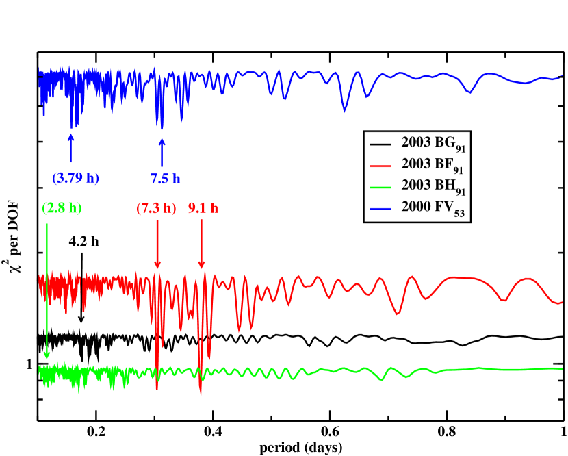
Figure 1: Periodogram for observed data. The best-fit periods (given in Table 5 and shown in Figure 2) are marked with the arrows, as are other peaks of note, in parentheses. 2003 BG₉₁ (black) has a suite of solutions, of which the best has a period of 4.2 hours; the others correspond to periods of 4.5 and 4.9 hours. 2003 BF₉₁ (red) has a secondary, non-resonant peak at 7.3 hours that is nearly as satisfactory a fit as the best fit. The best-fit solution for 2003 BH₉₁ (green) is not significant and is therefore marked in parentheses. The best-fit period for 2000 FV₅₃ (blue) is 7.5 hours; a solution that is nearly as significant is found with a period of 3.79 hours, almost exactly half the best-fit solution (see text).

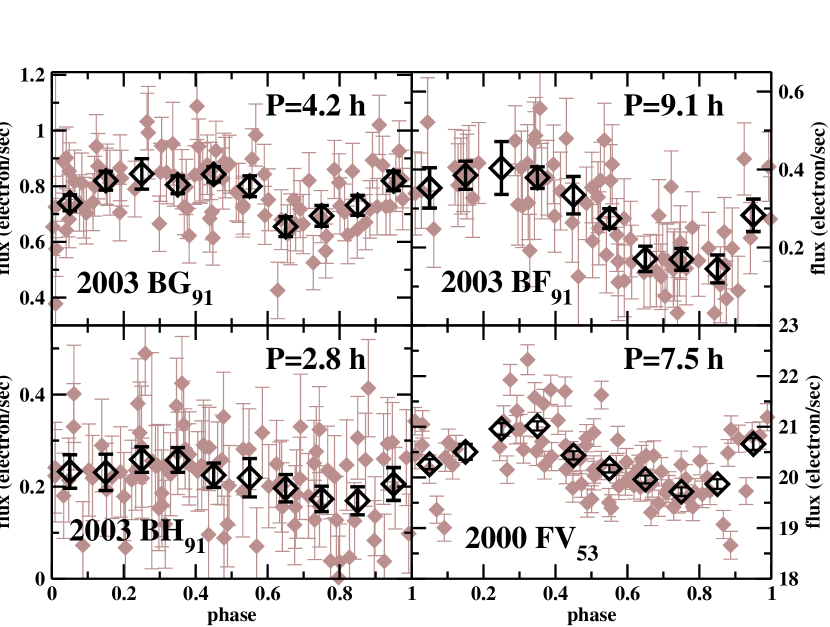
Figure 2: Data folded at best-fit periods (as labeled) as a function of phase. The pale, filled diamonds show the individual photometric measurements; the large, open symbols show the observed data binned with bins 0.1 phase units wide. The lightcurve amplitudes for 2003 BG₉₁, 2003 BF₉₁, and 2000 FV₅₃ are listed in Table 5. The best-fit solution for 2003 BH₉₁, with signifance of only 46%, is a period of 2.8 hours and amplitude of 0.42 magnitudes.

To determine the significance of each best-fit solution, we randomly scramble the time tags of the flux measurements for a given object and repeat the search for a best-fit sinusoid. For each KBO we fit 100 randomizations of the data, with the resulting best $\chi^{2}$/DOF of each trial plotted in Figure 3. Best-fit solutions to randomized 2003 BF₉₁ and 2000 FV₅₃ data are clearly less good than the best-fit solution to observed data at $>$99% confidence in both cases. The best-fit solution to the observed 2003 BG₉₁ data is marginally significant (90% confidence level), while the best fit for 2003 BH₉₁ data is no better than the best fits to randomized data.

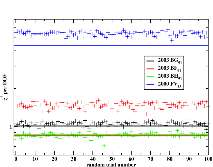
Figure 3: Significances of the best-fit solutions to (true) observed data (solid lines). We also show the $\chi^{2}$ per degree of freedom (DOF) for the best sinusoidal fit to each of 100 randomizations of each KBO’s true observed data (crosses). For 2003 BF₉₁ and 2000 FV₅₃, the true observed data are clearly significantly better fit by a sinusoid than are randomized versions of those data. The best fit for the true observed 2003 BG₉₁ data is marginally significant, and the 2003 BH₉₁ true observed data is not better fit than randomized data. Note that the vertical axis is logarithmic.

3.1 2003 BG₉₁

2003 BG₉₁ has a best-fit sinusoidal solution with a period of 4.2 hours and amplitude of 0.18 magnitudes. Similar, but less good, solutions are found for 4.5, 4.6, and 4.9 hours; these periods are not obviously aliases of each other. In the discussion that follows, we refer only to the best-fit period of 4.2 hours and, regardless of period solution, draw no significant conclusions about the internal properties of KBOs from this body’s lightcurve.

3.2 2003 BF₉₁

The periodogram for 2003 BF₉₁ shows two clear solutions that are nearly equivalently good fits: 9.1 hours and, secondarily, 7.3 hours (Figure 1). Both solutions have amplitudes of 1.09 magnitudes. The secondary peak is non-resonant with the best fit, i.e., not an obvious harmonic of the best-fit period, and is also quite significant compared to the randomized data. We therefore searched further for a best-fit solution that consisted of two independent sinusoids with independent phases, amplitudes, and periods, though the periods were restricted to a small range around each of best fits derived above. Formally, the $\chi^{2}$ improves significantly through allowing a two-sine fit, but the data may not warrant attaching too much importance to a multiple rotation pole interpretation. In the following analysis, we use the single-sinusoid better-fitting 9.1 hour period. None of our conclusions depend upon the choice between the two best-fit single-sinusoid periods, nor particularly on the choice of single- over double-sinusoid fit.

3.3 2003 BH₉₁

The best-fit sinusoid solution to the photometry of 2003 BH₉₁ has a period of 2.8 hours and amplitude of 0.42 magnitudes. However, the significance of this solution is only 46% when compared to 100 randomized trials of the 2003 BH₉₁ data. We therefore conclude that we failed to detect significant periodic variability for 2003 BH₉₁. To place an upper limit on the amplitude of an undetected periodic variation, we augmented the 2003 BH₉₁ data with synthetic lightcurves with various amplitudes and periods of 4 hours (a typical KBO photometric variation period) and carried out the best-fit solution search described above. We successfully recovered all synthetic lightcurves with amplitudes larger than around 15%. We can therefore place an upper limit on possible lightcurve amplitudes for 2003 BH₉₁, requiring that any such variation must have an amplitude less than 0.15 magnitudes to be undetected by us. The albedo variations and/or asphericity of this body must be less than 15%.

3.4 2000 FV₅₃

The best-fit solution for 2000 FV₅₃ gives a period of 7.5 hours. There is a peak of nearly equal significance at 3.79 hours, almost exactly half the best solution. The amplitude of the lightcurve is identical (0.07 mag) for both solutions. We compare the 2000 FV₅₃ observed data phased at each of these two periods in Figure 4. The phased data in the top panel appears double-peaked, with maxima at phases of 0.3–0.35 and 0.95–1.0. These two peaks have different shapes and are not 0.5 phase units apart, so we conclude that this lightcurve is double-peaked and non-sinusoidal, and that 7.5 hours is the true rotation period of 2000 FV₅₃. (We note a low-signal maximum for 2000 FV₅₃ in Figure 1 at 15 hours, which could be an alias of the 7.5 hour rotation period.) However, we include the 3.79 hour period in discussions below for completeness; this lightcurve (lower panel) is also significantly non-sinusoidal. Arguably, the true photometric period could be 3.79 hours, with 7.5 hours an alias of this true photometric period. We discuss the implications of the non-sinusoidal lightcurve below.

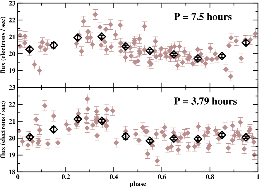
Figure 4: Observed data for 2000 FV₅₃ phased at the best-fit period of 7.5 hours (upper panel) and the second-best-fit period of 3.79 hours (lower panel), almost exactly half the best-fit period. In both panels the pale, filled diamonds show the individual photometric measurements; the large, open symbols show the observed data binned with bins 0.1 phase units wide. The amplitude of the lightcurve is identical (0.07 mag) for both solutions. The phased data in the top panel appears double-peaked, with maxima at phases of 0.3–0.35 and 0.95–1.0. These two peaks have different shapes and are not 0.5 phase units apart, so we conclude that this lightcurve is double-peaked and non-sinusoidal and that 7.5 hours is the true rotation period of 2000 FV₅₃. However, we include the 3.79 hour period in discussions below for completeness; this lightcurve (lower panel) is also significantly non-sinusoidal.

4 Lightcurve modulations produced by surface features

Observations of KBOs are necessarily conducted with the line of sight very close to the direction of illumination: in our case, 1$\fdg$4 and 1$\fdg$7 for the new bodies and 2000 FV₅₃, respectively. In this case we can ascribe lightcurve variations to some combination of (1) variation in surface composition and/or albedo that rotate through the observed hemisphere; (2) small-scale irregularities (“facets”) that rotate through (un-)favorable orientations for reflecting radiation to the observer; or (3) changes in projected area of the rotating body due to its gross shape, often approximated as an ellipsoid.

We will examine in turn these possible causes for the photometric variations of our measured KBOs, with the goal of extracting any possible constraints on their internal structure or surface composition. We will focus primarily on the objects 2003 BF₉₁ and 2000 FV₅₃ because their exceptionally large and small photometric variations, respectively, provide the most interesting constraints. The lightcurves of 2003 BG₉₁ and 2003 BH₉₁ are relatively unremarkable and do not help differentiate among possible physical models, so they will not be discussed further.

4.1 Albedo effects

If the large observed lightcurve variation of 2003 BF₉₁ is due entirely to albedo variations, surface patches with albedos that differ by a factor of 2.5 are required if the body has two distinct hemispheres and the rotation pole is perpendicular to the line of sight. If either of these two assumptions is relaxed, the required albedo range of the surface materials is even higher.

Little is known about KBO albedos. The few data points suggest a range from a few percent to perhaps 20% or more (Altenhoff et al., 2001; Jewitt et al., 2001; Groussin et al., 2003; Brown & Trujillo, 2004; Altenhoff et al., 2004; Noll et al., 2004b; Stansberry et al., 2004; Cruikshank et al., 2005; Stansberry et al., 2005). The canonical (but unsupported; see Altenhoff et al. (2004) and others) KBO albedo of 4%, which is based on comet albedos, is more than 4 times smaller than the 17% albedo observed for (55565) 2002 AW₁₉₇ (Cruikshank et al., 2005). This large albedo range could therefore plausibly exist on 2003 BF₉₁, though this possibility seems extreme and is not consistent with the existing sparse KBO albedo data. The range of albedos on Pluto’s surface exceeds a factor of 5 (Stern et al., 1997), although Pluto’s atmosphere contributes substantially to this effect and 2003 BF₉₁ would not be expected to have any atmosphere (because of its small size). The two hemispheres of Iapetus have albedos differing by a factor of 7, though this is likely due both to being tidally locked to Saturn and to contamination from other satellites.

These considerations favor shape over albedo as the primary cause of the variability of 2003 BF₉₁, more so because the main-belt asteroid (243) Ida provides a (rocky) example of the shape needed to produce this light curve (§6.4).

On the other hand, albedo and shape could be correlated, as would be the case with a large, fresh, bright crater. Furthermore, a crater or albedo feature could potentially dominate the majority of a hemisphere of a small body like 2003 BF₉₁, so we cannot exclude the possibility of a wide range of surface reflectance on 2003 BF₉₁. Additionally, KBO surfaces likely incorporate volatiles that could potentially be mobilized either through collisions or potentially even seasonal thermal variations. Migration of volatiles could plausibly create patchy surfaces with albedo variations.

The small photometric variations for the other three bodies could easily be explained by albedo variations on the surface. We note that lightcurves from albedo variations need not be symmetric, and the non-sinusoidal lightcurve of 2000 FV₅₃ suggests the rotation of (two) bright spots past the subobserver point. However, it is unlikely that albedo variations would conspire to reduce the amplitude of an otherwise large, shape-derived light curve (this would require a dark long axis and bright short axis of an elongated rotating body). Therefore, the possibility of albedo variation does not invalidate the geophysical arguments presented below.

4.2 Facets on KBOs

A second possible explanation of the KBO lightcurves arises from study of small bodies of the inner Solar System. Complex shape models have been determined for a number of asteroids and near Earth objects (NEOs) not only from spacecraft observations (e.g., Thomas et al. (1999); Wilkison et al. (2002)) but also from radar studies (see Ostro et al. (2002) for a review). Good lightcurves have been measured for many asteroids and NEOs whose shapes are known, and several NEOs are observed to have lightcurve amplitudes substantially larger or smaller than their elongated shapes naively would suggest (Pravec et al., 1998; Benner et al., 1999, 2002).

Because asteroids, KBOs, and comets all are heavily cratered bodies, non-uniform facets (reflecting faces and partially concave shapes) potentially can mask the true shape of the body. The scenario in which faceted KBOs show lightcurves larger than their gross shape would otherwise suggest cannot be ruled out. Thus, 2003 BF₉₁ could have a complicated topography that produces a lightcurve that — at least during our observing season — is substantially larger than its gross shape might otherwise indicate. Conversely, the gross shape of 2000 FV₅₃ may be less regular than its small amplitude light curve suggests, a caveat to bear in mind for the analyses below. Facets on 2000 FV₅₃ could also produce the observed non-sinusoidal lightcurve.

5 Geophysical considerations

In this section we regard the photometric variation as primarily a result of the gross shape of the KBO, and examine the constraints on internal strength and density that may be derived from the rotation properties. We will focus primarily on the constraints imposed by the small 0.07 mag amplitude of the 2000 FV₅₃ lightcurve.

5.1 A simple shape model

Observed KBO brightness variations may be the result of the gross aspherical shape of the body. A KBO may generally be thought of as having three primary axes, $a$, $b$, and $c$, where $a\geq b\geq c$ and where rotation takes place about $c$ in the minimized energy and angular momentum state. If this body is viewed equatorially, the ratio $a/b$ determines the magnitude of the observed lightcurve modulation as $\Delta m=2.5\log(a/b)$. Lacerda & Luu (2003) present a formalism for calculating an observed magnitude variation (for essentially Lambertian bodies) as a function of body shape and the viewing angle $\theta$ between the rotation axis and the (coincident) lines of sight and illumination (their Equation 2). The conditions in which amplitudes smaller than 0.07 mag are produced correspond to bodies of any shape seen nearly pole-on ($\theta\approx 0$); and nearly spherical bodies ($a\approx b\approx c$) seen at any angle. Note that for a KBO in pole-on rotation, the coincidence of illumination, line-of-sight, and rotation axes drives the lightcurve amplitude to zero regardless of the body shape or surface properties. In this configuration, the low amplitude of the 2000 FV₅₃ lightcurve would allow no definitive constraints on its properties (although a useful constraint can still be derived from the photometric period; see below). If 2000 FV₅₃ is significantly aspherical and exactly pole-on at present, its lightcurve amplitude should increase as it proceeds along its 250 year orbit; a 20 year observational baseline could provide a pole-Earth angle change of $\sim$30 degrees, potentially revealing the equatorial aspect and therefore shape of the body. However, 2000 FV₅₃ was targeted without regard to variability properties, so we can consider its pole orientation to be a random variable. Rotation axes within 25° of pole-on occur less than 10% of the time for random orientations, so we will exclude as unlikely any solution that requires $\theta<25\arcdeg$. We note further that, of the 10 KBOs and Centaurs with $7.5\leq H\leq 9.5$ (that is, objects around the size of 2000 FV₅₃) and measured light curves, 4 have amplitudes $\leq 0.2$ mag (see Table 6.3). Low variability is therefore not rare in the 2000 FV₅₃ size range, consistent with the argument that the small 2000 FV₅₃ lightcurve need not be produced by an unlikely orientation.

If the small lightcurve is not produced by a nearly pole-on orientation, several approaches lead to interesting constraints on the physical properties of 2000 FV₅₃. We consider in turn the possibilities that 2000 FV₅₃ has essentially zero internal strength (a fluid); low internal strength (a rubble pile); or material strength as in a monolithic (consolidated) body.

5.2 Fluid solutions

Chandrasekhar (1969); Hubbard (1984); and Tassoul (2000) have discussed the energy distributions and shapes of rotating, equilibrium, fluid bodies, and we apply their analyses here. The physical state of a rotating, fluid (strengthless) body depends on the angular momentum and distribution of matter. Non- or slowly-rotating fluid bodies are generally spherical. Moderate rotation produces a Maclaurin spheroid in which $a=b\gtrsim c$, and faster rotation results in a triaxial Jacobian ellipsoid in which $a>b\gtrsim c$. Hubbard defines the dimensionless rotation rate $\Omega$ as

$$\Omega^{2}\equiv\frac{\omega^{2}}{2\pi G\rho}$$ (1)

where $\omega$ is the angular rotation rate and $\rho$ is the bulk density of the body; in this formalism, the transition from Maclaurin to Jacobian bodies occurs at the bifurcation point $\Omega^{2}=0.19$.

The maximum value for the dimensionless rotation rate ($\Omega$) is reached at the bifurcation point. Thus, the minimum density for a fluid 2000 FV₅₃ is 0.67 g cm^-3 for a rotation period of 7.5 hours. All densities greater than this produce two theoretically viable solutions, one representing the Jacobian ellipsoid branch of solutions and one the the Maclaurin spheroid branch. Here we consider each branch in turn.

5.2.1 Jacobian ellipsoid solution

If we assume that the observed 2000 FV₅₃ lightcurve is derived from the gross shape of the body, then we require the branch of solutions corresponding to a triaxial Jacobian ellipsoid where $a>b$. The rotation period must be 7.5 hours: if the best-fit solution of 7.5 hours is used, its double-peaked nature implies that it is a complete rotation period, whereas if the second-best-fit solution of 3.79 hours is used, its single peak implies that 3.79 hours corresponds to only a half period (since the lightcurve is shaped-derived for a Jacobian body). Hence, we know $\omega$ (the angular rotation rate). Tassoul introduces $\tau$, which describes the energy state of a rotating body and which is the ratio of rotational kinetic energy (K) to the absolute value of the gravitational potential energy (W): $\tau=K/|W|$, where $\tau$ is small for nearly spherical bodies and increases for bodies with increasing asphericities (Figure 5). Tassoul shows the relationship between $\Omega^{2}$ and $\tau$; from Equation 1 and our knowledge of $\omega$, we convert this relationship to $\rho$ as a function of $\tau$. This result — bulk density as a function of the energy state of the body for a Jacobian ellipsoid — is shown in Figure 5 as the red line on the right half of the plot.

Chandrasekhar (1969) tabulates the relationship between $b/a$, $c/a$ and $\omega^{2}/(\pi G\rho)$ (what Chandrasekhar writes as $\Omega$ we write here as $\omega$, the angular rotation rate). We therefore can derive the relationship between $b/a$, $c/a$, and $\rho$, and consequently between $b/a$, $c/a$, and $\tau$. From $b/a$ and the observed $\Delta m$, we calculate the required viewing angle $\theta$ following Equation 2 of Lacerda & Luu (2003), deriving $\theta$ as a function of $\tau$. Lastly, we introduce $L(\leq\theta)=(1-\cos\theta)$, which is the probability, from simple geometric arguments, that a randomly oriented rotation pole has an orientation angle less than or equal to $\theta$. We show $L(\leq\theta)$ as a function of $\tau$ in Figure 5.

We exclude $L(\leq\theta)<0.1$ solutions as improbable. For 2000 FV₅₃, $L(\leq\theta)\geq 0.1$ corresponds to $a/b=2.8$ and $a/c=3.3$ and to $\rho\leq 1.0$ g cm^-3 (Figure 5). Thus, for Jacobian solutions — the only fluid solutions in which the photometric lightcurve is derived from the gross aspherical shape of the body — the bulk density of 2000 FV₅₃ must be 0.67–1.0 g cm^-3 (red solid line in Figure 5).

By comparison, assigning Pluto’s density of 2 g cm^-3 (Tholen & Buie, 1997) to 2000 FV₅₃ and assuming a Jacobian solution, we find $a/b\approx 5.6$ and $a/c\approx 6.1$, a long, thin body whose shape would be the most extreme in the Solar System: asteroid 216 Kleopatra (the “dogbone asteroid”) has $a/b$ around 2.3 (Ostro et al., 2000; Hestroffer et al., 2002).

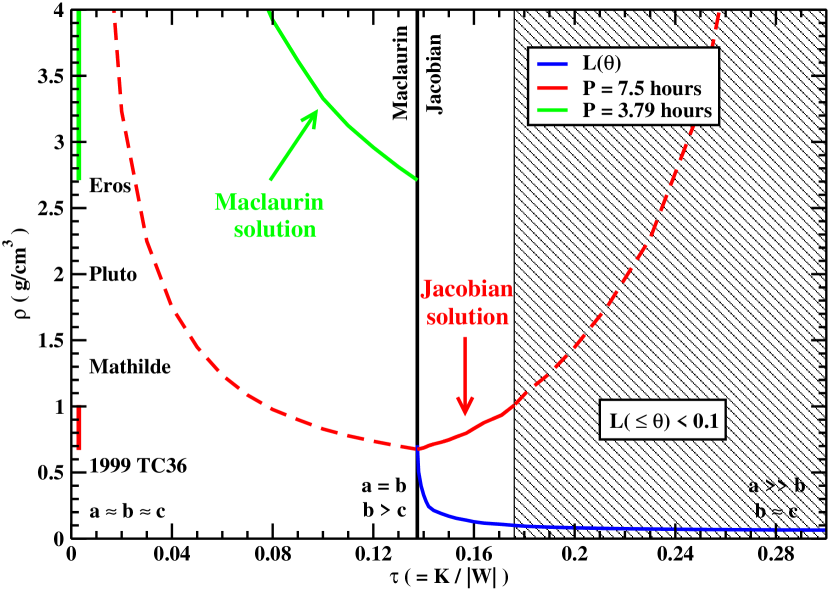
Figure 5: Density versus energy state for geophysical equilibrium fluid solutions for 2000 FV₅₃, where $\tau$ is the ratio of rotational kinetic energy (K) to the absolute value of the gravitational potential energy (W). The thick vertical line at $\tau=0.1375$ marks the bifurcation point between Maclaurian solutions and Jacobian solutions. Red curves show solutions for rotation a rotation period of 7.5 hours. The green curve shows the solution for a 3.79 hour period, possible in the Maclaurin branch. The blue curve shows $L(\leq\theta)$, the probability of the orientation required for a given $\tau$ (this probability is plotted between zero and one using the labels on the vertical axis). The grey hatched region indicates $L(\leq\theta)<0.1$, which we consider unlikely. The only likely Jacobian solutions (solid red line) have densities 0.67–1.0 g cm^-3 (as indicated by the red bar along the vertical axis). The right dashed red curve shows unlikely Jacobian solutions (low geometric probability). The left dashed red curve shows solutions that are unlikely because a double-peaked lightcurve is an unlikely to reflect the true rotational period of a Maclaurin body. Instead, the green curve shows the possible densities for Maclaurin solutions (indicated by the green bar along the vertical axis). The densities of asteroids Mathilde and Eros (Yeomans et al., 1997, 1999; Veverka et al., 1999), Pluto (Olkin et al., 2003), and KBO (47171) 1999 TC₃₆ (Stansberry et al., 2005) are indicated. The approximate relationships among $a$, $b$, and $c$ are given to lend intuition to the solution shapes described.

5.2.2 Maclaurin spheroid solutions

The Maclaurin branch of solutions represents oblate spheroids with $a=b$ and rotation about $c$. In this scenario, there is no modulation of cross-sectional area during rotation. Here, photometric variations must be due to surface features, either albedo variations (Section 4.1) or facets (Section 4.2). The rotation period for 2000 FV₅₃ could therefore be the second-best-fit solution of 3.79 hours, as a double-peaked lightcurve (i.e., the 7.5 hour period) would have to be produced by the unlikely configuration of bright (or dark) spots on opposite hemispheres of a body. We show the solution for a 3.79 hour rotation period in green in Figure 5; the minimum allowable density is 2.7 g cm^-3, slightly higher than that of the (presumed rocky) NEO 433 Eros. Though there is formally no maximum, densities larger than 4 g cm^-3 are remarkably unlikely.

If 2000 FV₅₃ is a Maclaurin body with a double-peaked lightcurve and rotation period of 7.5 hours – a situation we consider unlikely because of the requirement that like surface features be antipodal, a seemingly improbable configuration – then the red dashed line on the left half of Figure 5 obtains.

5.2.3 Summary of fluid solutions

To summarize, if 2000 FV₅₃ is strengthless (fluid), there are two primary solutions, both of which would be surprising: (1) 2000 FV₅₃ is a triaxial body with $\rho$ in the range 0.67–1.0 g cm^-3, implying a very high ice fraction or very high porosity; or (2) 2000 FV₅₃ is an oblate spheroid with a “bright spot” (or else in an unlikely pole-on orientation) and has density $\rho\geq 2.7$ g cm^-3, which is quite high for a body that is expected to be rock and ice with moderate porosity. We are forced to conclude that a strengthless 2000 FV₅₃ must have a composition that is either surprisingly ice-rich or surprisingly rock-rich, implying that it is a fragment of a differentiated body. However, the (implied) sphericity and relatively large size of 2000 FV₅₃ do not favor the fragment interpretation.

Geophysical fluid solutions for 2003 BF₉₁ place no surprising constraints on its density: for Jacobian solutions, density is in the expected range 0.5–2.5 g cm^-3, and for the “Maclaurian-with-a-spot” model, the lower limit the density is 0.5 g cm^-3.

5.3 KBOs with non-zero internal friction

In the previous section, we found that the fluid solutions for 2000 FV₅₃ require surprising densities (or may be geometrically unlikely). However, if KBOs are rubble piles made of rocks and ice, we can relax the fluid assumption by allowing these rotating bodies to have intrinsic strength.

Holsapple (2001) has studied the effects on body shapes and rotation rates of allowing cohesionless rubble piles to experience internal friction akin to the strength exhibited by a pile of sand. The results are described in terms of $\phi$, the angle of internal friction (or angle of repose). Fluids necessarily have $\phi=0^{\circ}$; typical terrestrial soils have $\phi\lesssim 30^{\circ}$. Allowing bodies to have non-zero internal friction allows shapes that depart from the Maclaurin-Jacobian spheroid/ellipsoid sequence. We must assume a density to constrain internal friction; we first consider 2000 FV₅₃ and assume $\rho=1$ g cm^-3.

We consider the prolate spheroid case $a>b=c$ (e.g., Holsapple Figures 3 and 5), assumed to be rotating about $c$ with a rotation period of 7.5 hours. Holsapple assumes equatorial viewing, which we are not restricted to in our analysis. Instead we may consider a range of axis ratios, where each value of $b/a$ implies a specific viewing angle $\theta$ as constrained by the observed lightcurve amplitude. Holsapple’s dimensionless rotation rate (which he defines as $\Omega=\omega/\sqrt{\rho G}$) is determined by our assumption of $\rho$ and knowledge of $\omega$. If we require $L(\leq\theta)\geq 0.10$, then $b/a$ for 2000 FV₅₃ must be in the range 0.36–0.93. Throughout this range, $\phi\approx 5^{\circ}$ (Figure 6).

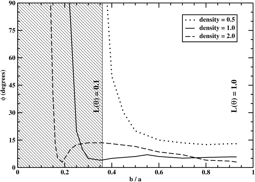
Figure 6: Angle of internal friction $\phi$ as a function of axis ratio $b/a$ for 2000 FV₅₃, for three different densities (as shown). These curves are slices through a complicated, undulating surface (see Holsapple Figure 3). Each value of $b/a$ implies a specific viewing angle $\theta$, as constrained by the observed lightcurve amplitude; $L(\leq\theta)<0.1$ for $b/a<0.36$ (hatched region). For densities of 1 or 2 g cm^-3, $\phi$ is less than around 15° throughout the region of probable orientation. However, $\rho=0.5$ g cm^-3 requires solutions with large $\phi$ for probable orientations. Therefore, densities much smaller than 1 g cm^-3 may be unlikely, but densities of 1–2 g cm^-3 provide solutions with reasonable angles of internal friction.

We now relax our density assumption. Carrying out the same analysis for $\rho=2.0$ g cm^-3, we find that $\phi$ is less than 15^∘ for all orientations with $L(\leq\theta)\geq 0.10$ (Figure 6). However, for $\rho=0.5$ g cm^-3, the minimum $\phi$ is around 13^∘ and probable orientations require large $\phi$.

We thus find that the internal friction for 2000 FV₅₃ can reasonably be small but non-zero. Additionally, densities much less than 1 g cm^-3 have solutions that increasingly require $\phi>30^{\circ}$, an unlikely physical scenario. Therefore, the physical picture that emerges is the following: 2000 FV₅₃ can readily be a rubble pile with density 1–2 g cm^-3 and small angles of internal friction. This solution does not require excessive porosity (from density estimates). This weak rubble pile body — multiply impacted into a collection of blocks that has only small internal friction – may be nearly, but not quite, relaxed to geophysical fluid equilibrium configuration. This interpretation also allows for the non-sinusoidal lightcurve observed for 2000 FV₅₃ is the body may still contain blocks that are out of fluid equilibrium.

For 2003 BF₉₁, $\rho=0.5$ g cm^-3 produces solutions for $\phi$ of generally less than 15 degrees. 2003 BF₉₁ solutions for $\rho=1.0$ and 2.0 g cm^-3 increasingly include $\phi$ of 18–25 degrees as well as narrow regions (in $b/a$) of acceptably low internal friction and very high internal friction (see Holsapple Figure 3). We conclude that no combination of density and internal friction are precluded for 2003 BF₉₁, though $\phi$ of 25 degrees is larger than is observed for most asteroids (Holsapple, 2001). This may indicate that 2003 BF₉₁ is more likely to be kept out of equilibrium by monolithic strength (see below) than by rubble-pile friction.

5.4 Material Strength

We considered above small-grained rubble piles, gravitational aggregates of loose material (see, e.g., Leinhardt et al. (2000)). Rubble pile bodies can also have “strength” if they consist of some large blocks in a mixture of smaller rubble (D. Richardson, pers. comm.; Richardson et al. (2005)). Finally, small bodies in the Solar System can be strong if they are monolithic bodies – essentially a single chip or fragment from a larger body, or the frozen remnant of a previously fluid body. In theory, such bodies could be either rock or ice.

2000 FV₅₃ may be far from an equilibrium rotation configuration if it is composed of one (or a few) blocks of solid material. Surface gravity scales linearly with the product of size and density; using this rough guideline, topography on 2000 FV₅₃ on the order of 10 km (enough to create 10% asymmetries) could easily be supported by strength (E. Apshaug, pers. comm.). If monolithic strength exists on 2000 FV₅₃ and supports topography, though, then the question exists why 2000 FV₅₃ is nearly symmetric as its lightcurve suggests. Additionally, dynamical arguments (see below) suggest a much-impacted and therefore completely shattered and rubble-like body. Irregular surface topography – that need not be supported by monolithic strength and is similar to the facets discussed above – could produce the non-sinusoidal lightcurve observed for 2000 FV₅₃.

The pressure at the center of a planetary body may be approximated as $GM^{2}/r^{4}$ where $M$ and $r$ are the mass and radius of the body. When $b/a$ for 2003 BF₉₁ is in the range 0.3–0.9, the overburden pressure produced by the asymmetric shape is 1–10 kilobars. The strength of clean laboratory ice is approximately 10 kilobars and that of snow is 0.01–0.1 kilobars (E. Asphaug, pers. comm.). Thus, the central stress in 2003 BF₉₁ could easily be supported by its material strength. 2003 BF₉₁ could easily be a rotating, coherent monolith with a substantially aspherical shape.

6 Discussion

6.1 Summary of Constraints

2000 FV₅₃ is a modest-sized KBO of diameter 116 km if the albedo is 0.10. There is a small chance that the low amplitude of the 2000 FV₅₃ light curve is attributable to pole-on rotation, but otherwise it must be a remarkably spherical body. Topography is allowed by strength arguments, but the size of 2000 FV₅₃ suggests that it should have been impacted many times (Durda & Stern (2000); see below) and hence be a rubble pile, not a monolithic body. The solutions for a fluid body require either a surprisingly low ($<$1 g cm^-3) or high ($>$2.7 g cm^-3) density, likely requiring 2000 FV₅₃ to be a remnant of a differentiated body. The former solution may imply a remarkably large porosity.

A more plausible solution is that 2000 FV₅₃ is a rubble pile of density 1–2 g cm^-3, held slightly out of the minimum-energy shape by internal friction among constituent blocks that are relatively small. The non-sinusoidal light curve of 2000 FV₅₃ requires surface inhomogeneity or a departure from ellipsoidal shape, but either effect need only be slight, and the latter is easily allowed for by a nearly-relaxed rotating body with non-zero internal friction.

The flux from the small body 2003 BF₉₁ (20 kilometers diameter, for albedo of 10%) varies by a factor $>$2.5 over the light curve. Such large-amplitude variation is achievable if the body is an irregularly-shaped collisional remnant consisting of one or a small number of coherent fragments supported by material strength. Alternately, extreme albedo variations would be required to explain the 1.09 mag lightcurve variation, perhaps with one impact-generated clean ice hemisphere contrasting with a darker (5%–10% albedo, consistent with that measured for other KBOs and Centaurs) hemisphere.

The ACS data for 2003 BG₉₁ and 2003 BH₉₁ do not allow placing any interesting constraints on surface or internal composition.

6.2 Collisions in the Kuiper Belt

The Kuiper Belt is generally thought of as a collisionally evolved population. This environment can readily produce facets on KBOs; impacts likely can also produce albedo features on KBOs through cratering; and elongated objects can be produced through fragmentation. However, the nearly spherical 2000 FV₅₃ must also be created through, or survive, collisional evolution.

Durda & Stern (2000) have calculated the timescale for disruptive collisions based on the present environment in the Kuiper Belt and assuming the pre-Bernstein et al. (2004) understanding (i.e., overestimation) of the small-end size distribution. They found that the timescale for disrupting a 100 km KBO is substantially longer than the age of the Solar System. Thus, 2000 FV₅₃ is likely not a fragment that was recently created. Instead, the size of 2000 FV₅₃ likely records the timescale and efficiency of accretion in the Kuiper Belt: 2000 FV₅₃ represents an intermediate product of the accretion process that formed Kuiper Belt giants like Quaoar and Pluto. Leinhardt et al. (2000) showed that pairwise accretion of rubble piles can produce both spherical and aspherical bodies. Thus, both 2000 FV₅₃ and Quaoar, which potentially has a 10% asphericity as indicated by its lightcurve (Ortiz et al., 2003b), can have gross shapes that are the direct result of rubble pile accretion. Additionally, 2000 FV₅₃ may have been impacted many times since its formation, resulting in a completely shattered body (consistent with Pan & Sari (2005)); we note that early in the Solar System’s history, the space density of bodies in the Kuiper Belt was higher than today and the impact rate was higher than at present. Multiple collisions can produce the small internal friction values we derived in Section 5.3. A consistent picture for 2000 FV₅₃ is therefore that of a body that accreted to approximately its present size; has been substantially shattered due to extensive collisions; has little internal friction due to its rubble pile nature; and is nearly, but not completely, relaxed, thus nearly attaining a rotating fluid equilibrium state.

Durda & Stern (2000) find that the disruption timescale for a 30 kilometer body is also longer than the Solar System, implying that formally a 30-km KBO would reflect primordial growth, not collisional disruption. Including the Bernstein et al. (2004) results will increase the disruption timescale for bodies of this size because of the dearth of small bodies. Thus, the picture for 2003 BF₉₁ may be somewhat complicated, as an elongated body is implied by its lightcurve amplitude. 2003 BF₉₁ may be a fragment from an unusual, but not wildly improbable, collision between 50–100 kilometer bodies. Furthermore, this collision could have occured billions of years ago when the space density of KBOs was higher, before later dynamical sculpting and mass loss (e.g., Morbidelli et al. (2003); Gomes et al. (2005)). Our interpretation of the 2003 BF₉₁ data is that the body is an elongated KBO (though not necessarily a monolithic body), and the collisional fragment solution is appealing in this case.

Alternately, 2003 BF₉₁ may have a complicated surface that produces a lightcurve larger than its gross shape would suggest. Eons of impacts certainly could produce arbitrarily complicated surface topographies, though Korycansky & Asphaug (2003) show that cumulative small impacts on rotating asteroids tend to lead to oblate shapes, which cannot produce the observed lightcurve. Understanding this object, in the absence of many comparably small KBOs, requires us to look elsewhere in the Solar System (Section 6.4).

6.3 Comparison to other KBOs

We list in Table 6.3 the 65 KBOs and Centaurs (excluding comets) for which lightcurve measurements or upper limits have been published; 37 of these have reported periodic lightcurve amplitudes, typically greater than $\sim$0.1 magnitudes. Most of these bodies have implied rotational periods (or half-periods for double-peaked lightcurves) in the range 3–10 hours, similar to the periods derived for our HST/ACS KBO observations. Note that these surveys certainly do not represent a complete nor random sample: some non-detections are likely unreported, and these observations represent mostly the brightest (largest) KBOs, so biases certainly exist in this compiled literature sample. Nevertheless, interesting results can be derived.

The amplitude we derive for 2003 BF₉₁, together with the recently measured amplitude of 1.14 mag for 2001 QG₂₉₈ (Sheppard & Jewitt, 2004), are the largest amplitude variations (to date) for KBOs and Centaurs. Additionally, our data show lightcurves for the faintest (and therefore smallest) KBOs, to date. However, neither the large lightcurve amplitude of 2003 BF₉₁ nor the fact that the small bodies 2003 BF₉₁ and 2003 BG₉₁ have lightcurves are particularly remarkable in the Solar System, as many small asteroids are known to have lightcurve variations larger than 1 magnitude, including some kilometer-sized NEOs (Pravec et al., 2002).

Table 6: KBO and Centaur lightcurve data

Desig.	Number	Name	Period(s)	Amplitude(s)	H	References
			(hours)	(mag)
$\cdots$	$\cdots$	Pluto	153.6	0.33	-1	1
2003 EL61	$\cdots$	$\cdots$	3.9	0.28	0.1	2
$\cdots$	$\cdots$	Charon	153.6	0.08	1	1
2003 VB12	90377	Sedna	10.3	0.02	1.6	3
2002 LM60	50000	Quaoar	17.7	0.13	2.6	4
2001 KX76	28978	Ixion	$\cdots$	$<$0.05	3.2	5
2002 TX300	55636	$\cdots$	7.89, 8.12, 12.10	0.08, 0.09	3.3	5,6
2002 UX25	55637	$\cdots$	$\cdots$	$<$0.06	3.6	5
			14.4, 16.8	0.2	3.6	7
2000 WR106	20000	Varuna	6.34	0.42	3.7	8,9
2003 AZ84	$\cdots$	$\cdots$	6.72	0.14	4.0	5
2001 UR163	42301	$\cdots$	$\cdots$	$<$0.08	4.2	5
1996 TO66	19308	$\cdots$	3.96	0.26	4.5	5
			6.25	0.12, 0.33	4.5	10
1999 DE9	26375	$\cdots$	$\cdots$	$<$0.10	4.7	9
2000 EB173	38628	Huya	$\cdots$	$<$0.06	4.7	9
			6.75	$<$0.1	4.7	11
2001 QF298	$\cdots$	$\cdots$	$\cdots$	$<$0.12	4.7	5
1995 SM55	24835	$\cdots$	4.04	0.19	4.8	5
1998 WH24	19521	Chaos	$\cdots$	$<$0.10	4.9	9
1999 TC36	47171	$\cdots$	$\cdots$	$<$0.06	4.9	5
2000 YW134	82075	$\cdots$	$\cdots$	$<$0.1	5.1	5
1996 GQ21	26181	$\cdots$	$\cdots$	$<$0.10	5.2	9
1997 CS29	79360	$\cdots$	$\cdots$	$<$0.08	5.2	9
2002 VE95	55638	$\cdots$	$\cdots$	$<$0.06	5.3	5
1996 TL66	15874	$\cdots$	$\cdots$	$<$0.06	5.4	12
2001 CZ31	$\cdots$	$\cdots$	$\cdots$	$<$0.20	5.4	9
2001 QT297	88611	$\cdots$	$\cdots$	$<$0.15	5.5	13
2001 KD77	$\cdots$	$\cdots$	$\cdots$	$<$0.07	5.6	5
1998 SM165	26308	$\cdots$	4.00	0.56	5.8	14
1998 SN165	35671	$\cdots$	5.03	0.15	5.8	15
1999 KR16	40314	$\cdots$	5.93, 5.84	0.18	5.8	9
2000 GN171	47932	$\cdots$	8.33	0.61	6.0	9
1998 XY95	$\cdots$	$\cdots$	$\cdots$	$<$0.1	6.2	16
2001 FP185	82158	$\cdots$	$\cdots$	$<$0.06	6.2	5
2001 FZ173	82155	$\cdots$	$\cdots$	$<$0.06	6.2	9
2001 QG298	$\cdots$	$\cdots$	6.89	1.14	6.3	17
2001 QT297B	88611B	$\cdots$	4.75	0.6	$\sim$6.3	13
1996 TS66	$\cdots$	$\cdots$	$\cdots$	$<$0.16	6.4	12
1997 CU26	10199	Chariklo	$\cdots$	$<$0.1	6.4	18
1977 UB	2060	Chiron	5.92	0.09	6.5	19
1998 VG44	33340	$\cdots$	$\cdots$	$<$0.10	6.5	9
1996 TP66	15875	$\cdots$	$\cdots$	$<$0.04	6.8	20
1993 SC	15789	$\cdots$	$\cdots$	$<$0.04	6.9	12
1992 AD	5145	Pholus	9.98	0.15–0.60	7.0	21,22,23
1994 VK8	19255	$\cdots$	3.9, 4.3, 4.7, 5.2	0.42	7.0	12
1996 TQ66	$\cdots$	$\cdots$	$\cdots$	$<$0.22	7.0	12
1994 TB	15820	$\cdots$	3.0, 3.5	0.26, 0.34	7.1	12
1998 BU48	33128	$\cdots$	4.9, 6.3	0.68	7.2	9
2002 CR46	42355	$\cdots$	$\cdots$	$<$0.05	7.2	5
1997 CV29	$\cdots$	$\cdots$	16	0.4	7.4	24
1995 QY9	32929	$\cdots$	3.5	0.60	7.5	12
1998 HK151	91133	$\cdots$	$\cdots$	$<$0.15	7.6	9
2000 QC243	54598	Bienor	4.57	0.75	7.6	11
1995 DW2	10370	Hylonome	$\cdots$	$<$0.04	8.0	12
2000 FV53	$\cdots$	$\cdots$	7.5	0.07	8.2	this work
2002 PN34	73480	$\cdots$	4.23, 5.11	0.18	8.2	11
1999 TD10	29981	$\cdots$	15.45	0.65	8.8	11,25,26
1995 GO	8405	Asbolus	4.47	0.55	9.0	18,27
2001 PT13	32532	Thereus	8.3	0.16	9.0	11,28
2002 GO9	83982	$\cdots$	6.97, 9.67	0.14	9.3	11
2000 EC98	60558	$\cdots$	26.8	0.24	9.5	7
1993 HA2	7066	Nessus	$\cdots$	$<$0.2	9.6	18
1999 UG5	31824	Elatus	13.25	0.24	10.1	29
2003 BG91	$\cdots$	$\cdots$	4.2	0.18	10.7	this work
1998 SG35	52872	Okyrhoe	16.6	0.2	11.3	30
2003 BF91	$\cdots$	$\cdots$	9.1, 7.3	1.09	11.7	this work
2003 BH91	$\cdots$	$\cdots$	$\cdots$	$<$0.15	11.9	this work

References. — (1) Buie et al. (1997); (2) Rabinowitz et al. (2005); (3) Gaudi et al. (2005); (4) Ortiz et al. (2003b); (5) Sheppard & Jewitt (2003); (6) Ortiz et al. (2004); (7) Rousselot et al. (2005); (8) Jewitt & Sheppard (2002); (9) Sheppard & Jewitt (2002); (10) Hainaut et al. (2000); (11) Ortiz et al. (2003a); (12) Romanishin & Tegler (1999); (13) Osip et al. (2003) (14) Romanishin et al. (2001); (15) Peixinho et al. (2002); (16) Collander-Brown et al. (2001); (17) Sheppard & Jewitt (2004) (18) Davies et al. (1998); (19) Bus et al. (1989); (20) Collander-Brown et al. (1999); (21) Buie & Bus (1992); (22) Farnham (2001); (23) Tegler et al. (2005); (24) Chorney & Kavelaars (2004); (25) Rousselot et al. (2003); (26) Choi et al. (2003): (27) Kern et al. (2000); (28) Farnham & Davies (2003); (29) Gutiérrez et al. (2001); (30) Bauer et al. (2003)

Note. — Multiple measurements have been made for several bodies. For non-detections, we cite here only the most sensitive measurement. For lightcurve determinations that are in agreement with each other, we cite all references on the same line. For lightcurve determinations that disagree where there is not clearly a superior measurement, we list the conflicting results on separate lines. Data reported here for the first time are shown in bold.

Pravec & Harris (2000) derive a simple expression that approximates the critical (minimum) period ($P_{c}$, in hours) for a rotating body as a function of density and lightcurve amplitude (in magnitudes):

$$P_{c}\approx 3.3\sqrt{\frac{1+\Delta m}{\rho}}.$$ (2)

This relation assumes a fluid body, that is, $\phi=0$. Although more rigorous treatments of lightcurve data are possible, as shown above, we will here make this assumption to allow ready comparisons among bodies (and to the main belt asteroid and NEO populations). Following Pravec & Harris (2000), we plot lightcurve amplitudes and observed periods for all presently known KBO and Centaur data, including our new HST data for 2003 BF₉₁, 2003 BG₉₁, and 2000 FV₅₃ (Figure 7). The rotation periods of most KBOs and Centaurs could be either the observed photometric period (open circles in Figure 7) or twice the photometric period (closed symbols). For cases in which the true periods are known from double-peaked lightcurves, only this true period is plotted (closed symbol).

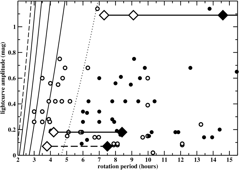
Figure 7: Amplitudes and periods for all KBOs and Centaurs (excluding comets) with observed lightcurve variations (data from Table 6.3). Large diamonds represent our HST observations and small circles are data from other sources. Open symbols indicate photometric periods; filled symbols indicate rotation periods that are twice the observed photometric period. Objects known to have double-peaked lightcurves are plotted only as filled symbols. Horizontal lines connect photometric and twice photometric solutions for our HST observations of 2003 BF₉₁, 2003 BF₉₁, and 2000 FV₅₃ (the horizontal line for 2000 FV₅₃ is dashed to suggest that the lightcurve likely is double-peaked and that the 3.79 hour solution is unlikely); similar lines could be drawn for most observations represented here, as most KBO lightcurves do not allow distinguishing between these two solutions, but we omit these connecting lines for other data for clarity. The curves represent solutions for critical rotation periods ($P_{c}$) for various densities (in g cm^-3): 0.5 (dotted line), 1, 1.5, 2, 2.5, and 3 (dashed) (from Equation 2). Regions above and to the left of a given curve are unstable for a given density. A maximum KBO density of 1.0–1.5 g cm^-3 (for single-peaked solutions) or perhaps 0.5 g cm^-3 (for double-peaked solutions) is suggested by the clustering of points up to but not beyond the curves for those densities. Compare to Figure 8 of Pravec & Harris (2000).

In Figure 7 we also show solutions corresponding to critical periods for densities spanning the range of plausible values for icy-rocky bodies. Remarkably, there is an apparent “rotation rate barrier” in that there appear to be no KBOs or Centaurs whose densities must be greater than 1 or 1.5 g cm^-3; this conclusion is derived from the case in which rotation periods are identical to photometric periods. Similarly, assuming that rotation periods are twice the photometric periods shows that there are no KBOs or Centaurs whose densities must be greater than 0.5 g cm^-3. This does not preclude larger densities, but means that no KBOs or Centaurs are observed to have rotations that require larger densities. Furthermore, Pravec & Harris (2000) interpret their results for NEOs by saying that the density that corresponds to the “rotation rate barrier” is likely the maximum bulk density for that population. While it seems unlikely that the maximum density for KBOs is less than 1 g cm^-3, it is nevertheless remarkable that no KBOs or Centaurs require densities larger than around 0.5 or 1.5 g cm^-3. For comparison, we note that (47171) 1999 TC₃₆ has a density around 0.5 g cm^-3 (Stansberry et al., 2005); that the “rotation rate barrier” for comets is around 0.6 g cm^-3 (Weissman et al., 2004); and that this “barrier” for NEOs is 2–3 g cm^-3 for bodies larger than 200 m (Pravec & Harris, 2000).

Since KBOs and Centaurs are expected to be a mixture of ice (density around 1 g cm^-3) and rock (density perhaps around 3 g cm^-3), we can roughly estimate that porosity may be important at the level of tens of percent (see below). A further implication is that KBOs and Centaurs in this size range generally may not have significant tensile strength, which would allow stable KBO solutions to the upper left of the critical lines shown in Figure 7 (recall that the discussion in Section 5.3 refers to cohesionless bodies). This is further confirmation that KBOs and Centaurs larger than 25 km diameter are likely to be rubble piles. Our general conclusion from this analysis — that the bulk densities of KBOs and Centaurs likely lie in the range 0.5–1.5 g cm^-3 — is not surprising and confirms results that we have shown above.

Finally, we note that the percentage of small KBOs with detected lightcurves is significantly greater than the percentage of large KBOs with detected lightcurves (Table 6.3). This is consistent with the arguments presented above: more small KBOs are likely to be fragments than large KBOs; fragments are more likely to be non-spherical than primordial bodies; lightcurves are likely to be produced by non-spherical bodies; therefore, a greater percentage of small KBOs should show significant lightcurve variations than large KBOs. We again restate that the data presented in Table 6.3 is certainly biased against null results and biased toward the detection of small amplitude lightcurves for big (but not small) KBOs. Nevertheless, if taken at face value, the data presented in Table 6.3 therefore supports the theoretical models described above, with the largest bodies remaining undisrupted since accretion and smaller bodies representing collisionally-derived fragments.

6.4 Comparison to other Solar System bodies

The KBOs and Centaurs shown in Figure 7 are generally hundreds of kilometers, as is 2000 FV₅₃, but 2003 BF₉₁ and 2003 BG₉₁ have diameters a factor of five smaller: gravity may be important in rounding bodies larger than a few hundred kilometers, but does not prohibit smaller bodies from maintaining various extreme shapes (e.g., Richardson et al. (2002)). Therefore, the same physical processes and interpretations may not be relevant across size regimes within the Kuiper Belt, and it is possible that better analogies of individual objects are found elsewhere in the Solar System, despite differing collision rates and ice/rock fractions.

Outer planet satellites may be useful analogies to hundred kilometer KBOs; indeed, some outer planet satellites may be captured KBOs (Johnson & Lunine, 2005). Jupiter’s moon Amalthea has $a/b=1.8$, $a/c$ around 2, and a derived density of less than 1.0 g cm^-3 (Anderson et al., 2005). (Compare this result to the plausible solutions for 2000 FV₅₃ shown in Figure 5.) The best interpretation for this modest-sized body — with mean radius around 80 km, Amalthea is very close in size to 2000 FV₅₃ — is a porosity of tens of percent even when the satellite is largely water ice. The physical state of this body is not presently understood, so we can draw no useful analogy from it, other than to say that extremely low densities in the Solar System (including 0.5 g cm³ for (47171) 1999 TC₃₆ (Stansberry et al., 2005)) appear to be just that: extreme, but not forbidden.

The maximum asphericity of 2000 FV₅₃ may be only a few percent (barring pole-on alignment or a pathological combination of dark surface regions along the long axis and bright surface regions along the short axis of an elongated body). The size of 2000 FV₅₃ is similar to a number of outer Solar System moons. Uranus’ moon Puck’s axis ratio is close to unity (Karkoschka, 2001), but all of these other satellites — which are presumably captured and perhaps fragments of disrupted bodies — are known to be at least 10% aspherically irregular, though we note that viewing geometries may play some role (outer planet satellites, except Uranus’, tend to be viewed close to equatorially, maximizing lightcurve variations, whereas KBOs are assumed to have randomized obliquities that are more likely to hide their true shapes). Furthermore, Sheppard & Jewitt (2002) compile a list of aspherical Solar System objects larger than 200 km and suggest that the four KBOs they observed to have lightcurve variations — all larger than 200 km — may also be irregular, with asphericities of tens of percent. It is thus remarkable that even modest asphericity of the 116 km 2000 FV₅₃ is unlikely based on our photometry (barring a pole-on orientation). Perhaps impacts have more thoroughly pulverized 2000 FV₅₃ (and KBOs) than satellites of giant planets. 2000 FV₅₃ would therefore have small internal friction and would be more relaxed and closer to the fluid equilibrium state. We note that approximately half of the KBOs that have been searched for photometric variability show no such signal, typically with sensitivities around 0.1 magnitudes. This 50% null result could be interpreted as suggesting that many hundred kilometer-sized KBOs are less than 10% aspherical. A significant difference between KBOs and outer Solar System satellites may be implied.

We can look to the comet population for relevant analogies for the smaller KBOs. Jewitt et al. (2003) studied shapes of comet nuclei, which are an order of magnitude smaller than the HST KBOs and two orders of magnitude smaller than most other well-studied KBOs. They conclude that the primary cause of comet nuclei asphericity likely is extensive mass loss. We suspect that such a process is not significant for classical KBOs, such as the four we observed with HST, that never approach closer to the Sun than $\sim$35 AU, but could be important for Centaurs, which can have semi-axes as small as $\sim$15 AU.

Weissman et al. (2004) compiled rotation periods and projected axis ratios ($a/b$) for 13 short-period comets and carried out an analysis similar to our Section 6.3 and Figure 7. They find an apparent “rotation rate barrier” that corresponds to an upper limit density around 0.6 g cm^-3, similar to the upper limit we derive from the double-period solutions for KBOs (filled circles in Figure 7). Comets clearly have non-gravitational forces (e.g., jets) that can affect both shape and rotation periods, so this apparent agreement should not be overemphasized. Nevertheless, the idea that short-period (Jupiter-family) comets derive from the Kuiper Belt (e.g., Levison & Duncan (1997)) may be supported by this agreement.

Finally, the asteroid belt includes bodies throughout the size range of KBOs and may prove useful for understanding the physical properties of KBOs. 2000 FV₅₃ has no good close analog among main belt asteroids (using absolute magnitude, lightcurve amplitude, and period as criteria). However, 2003 BF₉₁ may have a good and easily imagined analog in the main asteroid belt, based on lightcurve amplitude and approximate size: asteroid (243) Ida, which has maximum and minimum dimensions of 55.3 km and 14.6 km, asymmetry (area-weighted average of the ratio of the radii) of 1.48, and an observed lightcurve around 0.8 magnitudes (Simonelli et al., 1996; Thomas et al., 1996). Ida has clearly been much affected by disruptive collisions, as suggested by its membership in the Koronis dynamical family; by the presence of its (presumably impact-generated) satellite, Dactyl; and by its much-cratered appearance (Greenberg et al., 1996). All evidence suggests that Ida is a collisional fragment of the (former) Koronis parent body. Note that Ida’s significant aspect ratio demonstrates, at least in concept, that fragmentary results of collisional events can have substantially aspherical shapes and consequently large amplitude lightcurves. We note that the asteroid belt has a higher space density of bodies and larger impact speeds than the Kuiper Belt. Perhaps, however, it is not inappropriate to imagine an icy Ida when picturing 2003 BF₉₁.

7 Conclusions

We have derived best-fit lightcurves for four KBOs imaged in the HST/ACS KBO survey (Bernstein et al., 2004). 2003 BF₉₁ is found to experience large amplitude periodic brightness variations, whereas 2000 FV₅₃ significantly is found to undergo very small but non-zero amplitude periodic brightness variations that are non-sinusoidal. Our primary conclusions are the following:

• Plausibly, based on the range of suggested and measured albedos for KBOs, an albedo range of at least a factor of 2.5 could exist on 2003 BF₉₁, although such unlikely and extreme albedo ranges on single bodies in the outer Solar System are seen only in unusual situations. However, albedo and shape could be correlated, as would be the case with a large, fresh, bright crater. Furthermore it may be easier for a crater or albedo feature to dominate the majority of a hemisphere of a small body like 2003 BF₉₁, so we cannot exclude the possibility of a wide range of surface reflectance on 2003 BF₉₁.

• 2003 BF₉₁ could have complicated topography that produces lightcurves that — at least during our observing season — are substantially larger than their gross shapes might otherwise indicate. Facets on 2000 FV₅₃ could produce a small amplitude lightcurve that suggests a body more spherical than its true shape. Additionally, the relatively small deviations from sphericity required to produce the observed 2000 FV₅₃ lightcurve may be readily explained by topography – facets – in the presence of low surface gravity.

• The conditions in which small amplitude lightcurves are produced (e.g., 2000 FV₅₃) include bodies of any shape seen nearly pole-on ($\theta\approx 0$) and nearly spherical bodies ($a\approx b\approx c$) seen at any angle. For Jacobian solutions — the only non-pole-on fluid solutions in which the photometric lightcurve is derived from the gross aspherical shape of the body — the bulk density of 2000 FV₅₃ must be 0.67–1.0 g cm^-3. For Maclaurin solutions (rotating spot model) as well as for pole-on orientations, the minimum density is 2.7 g cm^-3.

  The simplest solution arises from allowing non-zero internal friction: 2000 FV₅₃ can readily be a rubble pile with density 1–2 g cm^-3 and small (but non-zero) internal friction.

The emerging picture for 2000 FV₅₃ is that of a body that accreted to approximately its present size; has been completely shattered due to extensive collisions; has little internal friction due to its rubble pile nature ($\phi$ small but likely non-zero); and is nearly, but not completely, relaxed, thus nearly attaining a rotating fluid equilibrium state. This conclusion is consistent with the idea that the timescale for disruptive collisions among 100 km KBOs is longer than the Solar System. The non-sinusoidal lightcurve could be produced by facets or surface topography, or simply as a result of 2000 FV₅₃ being nearly, but not quite, in rotational fluid equilibrium.

2003 BF₉₁ (as well as 2003 BG₉₁) is likely a single coherent fragment, the result of an unusual, but not wildly improbable, collision between 100 kilometer bodies.

We combine the new lightcurve data presented here with all other reported KBO photometry to understand the physical properties of the KBO population. Our general conclusion from this analysis is that the bulk densities of KBOs and Centaurs likely lie in the range 0.5–1.5 g cm^-3. This is consistent with the results of the detailed modeling we carried out for the HST/ACS KBOs and roughly consistent with the average bulk density for short-period comets. This agreement may strengthen the proposed genetic link between Kuiper Belt Objects and short-period comets. We furthermore show that the percentage of small KBOs with lightcurve variations is greater than that for large KBOs, implying that small KBOs are non-spherical fragments produced by collisions.

Outer Solar System satellites of the size of 2000 FV₅₃ almost all have asphericities greater than 10%. Perhaps 50% of similarly-sized KBOs show no variability at the 10% level, suggesting a significant difference between the evolutions of KBOs and outer Solar System satellites.

The most helpful and easily imagined Solar System analog for 2003 BF₉₁ may be the main belt asteroid (243) Ida, which has size, axis ratios, and shape that are similar to those we derive for 2003 BF₉₁. Ida has clearly been much affected by disruptive collisions and is a fragment of a larger parent body, further suggesting that 2003 BF₉₁ could be a collisionally shaped body. Perhaps it is not inappropriate to imagine an icy Ida when picturing the small KBO 2003 BF₉₁.

References

- Altenhoff et al. (2001) Altenhoff, W. J., Menten, K. M., & Bertoldi, F. 2001, A&A, 366, L9
- Altenhoff et al. (2004) Altenhoff, W. J., Bertoldi, F., & Menten, K. M. 2004, A&A, 415, 771
- Anderson et al. (2005) Anderson, J. D. et al. 2005, Science, 308, 1291
- Asphaug (2004) Asphaug, E. 2004, in Mitigation of Hazardous Impacts due to Asteroids and Comets, eds. M. Belton et al. (Cambridge: Cambridge University Press), 66
- Bauer et al. (2003) Bauer, J. M., Meech, K. J., Fernández, Y. R., Pittichova, J., Hainaut, O. R., Boehnhardt, H., & Delsanti, A. C. 2003, Icarus, 166, 195
- Bauer et al. (2004) Bauer, J. M., Buratti, B. J., Simonelli, D. P., & Owen, W. M., Jr. 2004, ApJ, 610, 57
- Benner et al. (1999) Benner, L. A. M. et al. 1999, Icarus, 139, 309
- Benner et al. (2002) Benner, L. A. M. 2002, M&PS, 37, 779
- Bernstein et al. (2004) Bernstein, G. M., Trilling, D. E., Allen, R. L., Brown, M. E., Holman, M., & Malhotra, R. 2004, AJ, 128, 1364
- Brown & Trujillo (2004) Brown, M. E. & Trujillo, C. 2004, AJ, 127, 2413
- Brownlee et al. (2004) Brownlee, D. E. et al. 2004, Science, 304, 1764
- Buie & Bus (1992) Buie, M. W. & Bus, S. J. 1992, Icarus, 100, 288
- Buie et al. (1997) Buie, M. W., Tholen, D. J., & Wasserman, L. H. 1997, Icarus, 125, 233
- Bus et al. (1989) Bus, S. J., Bowell, E., Harris, A. W., & Hewitt, A. V. 1989, Icarus, 77, 223
- Chandrasekhar (1969) Chandrasekhar, S. 1969, Ellipsoidal Figures of Equilibrium (New Haven: Yale University Press)
- Choi et al. (2003) Choi, Y. J., Brosch, N., & Prialnik, D. 2003, Icarus, 165, 101
- Chorney & Kavelaars (2004) Chorney, N. & Kavelaars, J. J. 2004, Icarus, 167, 220
- Collander-Brown et al. (1999) Collander-Brown, S. J., Fitzsimmons, A., Fletcher, E., Irwin, M. J., & Williams, I. P. 1999, MNRAS, 308, 588
- Collander-Brown et al. (2001) Collander-Brown, S. J., Fitzsimmons, A., Fletcher, E., Irwin, M. J., & Williams, I. P. 2001, MNRAS, 325, 972
- Cruikshank et al. (2005) Cruikshank, D. P., Stansberry, J. A., Emery, J. P., Fernández, Y. R., Werner, M. W., Trilling, D. E., & Rieke, G. H. 2005, ApJ, 624, 53
- Davies et al. (1998) Davies, J. K., McBride, N., Green, S. F., Mottola, S.. Carsenty, U., Basran, D., Hudson, K. A., & Foster, M. J. 1998, Icarus, 132, 418
- Durda et al. (1998) Durda, D. D., Greenberg, R., & Jedicke, R. 1998, Icarus, 135, 431
- Durda & Stern (2000) Durda, D. D. & Stern, S. A. 2000, Icarus, 145, 220
- Farnham (2001) Farnham, T. L. 2001, Icarus, 152, 238
- Farnham & Davies (2003) Farnham, T. L. & Davies, J. K. 2003, Icarus, 164, 418
- Fernández et al. (2002) Fernández, Y. R., Jewitt, D. D., & Sheppard, S. S. 2002, AJ, 123, 1050
- Gaudi et al. (2005) Gaudi, B. S., Stanek, K. Z., Hartman, J. D., Holman, M. J., & McLeod, B. A. 2005, ApJ, submitted
- Gomes et al. (2005) Gomes, R., Levison, H. F., Tsiganis, K., & Morbidelli, A. 2005, Nature, 435, 466
- Groussin et al. (2003) Groussin, O., Lamy, P., & Jorda, L. 2004, A&A, 413, 1163
- Greenberg et al. (1996) Greenberg, R., Bottke, W. F., Nolan, M., Geissler, P., Petit, J.-M., Durda, D. D., Asphaug, E., & Head, J. 1996, Icarus, 120, 106
- Gutiérrez et al. (2001) Gutiérrez, P. J., Ortiz, J. L., Alexandrino, E., Roos-Serote, M., & Doressoundiram, A. 2001, A&A, 371, L1
- Hainaut et al. (2000) Hainaut, O. R., Delahodde, C. E., Boehnhardt, H., Dotto, E., Barucci, M. A., Meech, K. J., Bauer, J. M., West, R. M., & Doressoundiram, A. 2000, A&A, 356, 1076
- Hestroffer et al. (2002) Hestroffer, D., Berthier, J., Descamps, P., Tanga, P., Cellino, A., Lattanzi, M., Di Martino, M., & Zappalà, V. 2002, A&A, 392, 729
- Holsapple (2001) Holsapple, K. A. 2001, Icarus, 154, 432
- Hubbard (1984) Hubbard, W. B. 1984, Planetary Interiors (New York: Van Nostrand Reinhold Company Inc.)
- Jewitt (1991) Jewitt, D. 1991, in Comets in the Post-Halley Era, eds. R. L. Newburn et al. (Dordrecht: Kluwer Academic Publishers), 19
- Jewitt et al. (2001) Jewitt, D., Aussel, H., & Evans, A. 2001, Nature, 411, 446
- Jewitt & Sheppard (2002) Jewitt, D. C. & Sheppard, S. S. 2002, AJ, 123, 2110
- Jewitt et al. (2003) Jewitt, D., Sheppard, S. S., & Fernández, Y. 2003, AJ, 125, 3366
- Karkoschka (2001) Karkoschka, E. 2001, Icarus, 151, 69
- Karkoschka (2003) Karkoschka, E. 2003, Icarus, 162, 400
- Kern et al. (2000) Kern, S. D., McCarthy, D. W., Buie, M. W., Brown, R. H., Campins, H., & Rieke, M. 2000, ApJ, 542, L155
- Korycansky & Asphaug (2003) Korycansky, D. G. & Asphaug, E. 2003, Icarus, 163, 374
- Kruse et al. (1986) Kruse, S., Klavetter, J. J., & Dunham, E. W. 1986, Icarus, 68, 167
- Lacerda & Luu (2003) Lacerda, P. & Luu, J. 2003, Icarus, 161, 174
- Leinhardt et al. (2000) Leinhardt, Z. M., Richardson, D. C., & Quinn, T. 2000, Icarus, 146, 133
- Levison & Duncan (1997) Levison, H. F. & Duncan, M. J. 1997, Icarus, 127, 13
- Morbidelli et al. (2003) Morbidelli, A., Brown, M. E., & Levison, H. F. 2003, EM&P, 92, 1
- Noll et al. (2002) Noll, K. S. et al. 2002, AJ, 124, 3424
- Noll et al. (2004a) Noll, K. S., Stephens, D. C., Grundy, W. M., & Griffin, I. 2004a, Icarus, 172, 402
- Noll et al. (2004b) Noll, K. S., Stephens, D. C., Grundy, W. M., Osip, D. J., & Griffin, I. 2004b, AJ, 128, 2547
- Olkin et al. (2003) Olkin, C. B., Wasserman, L. H., & Franz, O. G. 2003, Icarus, 164, 254
- Ortiz et al. (2003a) Ortiz, J. L., Gutiérrez, P. J., Casanova, V., Sota, A. 2003a, A&A, 407, 1149
- Ortiz et al. (2003b) Ortiz, J. L., Gutiérrez, P. J., Sota, A., Casanova, V., & Teixeira, V. R. 2003b, A&A, 409, L13
- Ortiz et al. (2004) Ortiz, J. L. et al. 2004, A&A, 420, 383
- Osip et al. (2003) Osip, D. J., Kern, S. D., & Elliot, J. L. 2003, EM&P, 92, 409
- Ostro et al. (2000) Ostro, S. J., Hudson, R. S., Nolan, M. C., Margot, J., Scheeres, D. J., Campbell, D. B., Magri, C., Giorgini, J. D., & Yeomans, D. K. 2000, Science, 288, 836
- Ostro et al. (2002) Ostro, S. J., Hudson, R. S., Benner, L. A. M., Giorgini, J. D., Magri, C., Margot, J. L., & Nolan, M. C. 2002, in Asteroids III, eds. W. F. Bottke, Jr. et al. (Tucson: University of Arizona Press), 151
- Pan & Sari (2005) Pan, M. & Sari, R. 2005, Icarus, 342, 348
- Peixinho et al. (2002) Peixinho, N., Doressoundiram, A., & Romon-Martin, J. 2002, New Astronomy, 7, 359
- Porco et al. (2003) Porco, C. C. et al. 2003, Science, 299, 1541
- Porco et al. (2005) Porco, C. C. et al. 2005, Science, 307, 1237
- Pravec et al. (1998) Pravec, P., Wolf, M., & arounová, L. 1998, Icarus, 136, 124
- Pravec & Harris (2000) Pravec, P. & Harris, A. W. 2000, Icarus, 148, 12
- Pravec et al. (2002) Pravec, P., Harris, A. W., & Michalowski, T. 2002, in Asteroids III, eds. W. F. Bottke, Jr. et al. (Tucson: Univ. Arizona Press), 113
- Rabinowitz et al. (2005) Rabinowitz, D. L., Barkume, K., Brown, M. E., Roe, H., Schwartz, M., Tourtellotte, S., & Trujillo, C. 2005, ApJ, submitted
- Richardson et al. (2002) Richardson, D. C., Leinhardt, Z. M., Melosh, H. J., Bottke, Jr., W. F., & Asphaug, E. 2002, in Asteroids III, eds. W. F. Bottke, Jr. et al. (Tucson: University of Arizona Press), 501
- Richardson et al. (2005) Richardson, D. C., Elankumaran, P., & Sanderson, R. E. 2005, Icarus, 173, 349
- Romanishin & Tegler (1999) Romanishin, W. & Tegler, S. C. 1999, Nature, 398, 129
- Romanishin et al. (2001) Romanishin, W., Tegler, S. C., Rettig, T. W., Consolmagno, G., & Botthof, B. 2001, BAAS, 33, 1031
- Rousselot et al. (2003) Rousselot, P., Petit, J.-M., Poulet, F., Lacerda, P., & Ortiz, J. 2003, A&A, 407, 1139
- Rousselot et al. (2005) Rousselot, P., Petit, J.-M., Poulet, F., & Sergeev, A. 2005, Icarus, 176, 478
- Samarasinha et al. (2004) Samarasinha, N. H., Mueller, B. E. A., Belton, M. J. S., & Jorda, L. 2004, in Comets II, eds. M. C. Festou et al. (Tucson: Univ. Arizona Press), 281
- Sheppard & Jewitt (2002) Sheppard, S. S. & Jewitt, D. C. 2002, AJ, 124, 1757
- Sheppard & Jewitt (2003) Sheppard, S. S. & Jewitt, D. C. 2003, Earth, Moon, & Planets, 92, 207
- Sheppard & Jewitt (2004) Sheppard, S. S. & Jewitt, D. C. 2004b, AJ, 127, 3023
- Simonelli et al. (1993) Simonelli, D. P., Thomas, P. C., Carcich, B. T., & Veverka, J. 1993, Icarus, 103, 49
- Simonelli et al. (1996) Simonelli, D. P., Veverka, J., Thomas, P. C., Helfenstein, P., Carcich, B. T., & Belton, M. J. S. 1996, Icarus, 120, 38
- Stansberry et al. (2004) Stansberry, J. A. et al. 2004, ApJS, 154, 463
- Stansberry et al. (2005) Stansberry, J. A. et al. 2005, submitted
- Stephens & Noll (2005) Stephens, D. C. & Noll, K. S. 2005, AJ, in press
- Stern et al. (1997) Stern, S. A., Buie, M. W., & Trafton, L. M. 1997, AJ, 113, 827
- Tassoul (2000) Tassoul, J.-L. 2000, Stellar Rotation (Cambridge: Cambridge University Press)
- Tegler et al. (2005) Tegler, S. C., Romanishin, W., Consolmagno, G. J., Rall, J., Worhatch, R., Nelson, M., & Weidenschilling, S. 2005, Icarus, 175, 390
- Tholen & Buie (1997) Tholen, D. J. & Buie, M. W. 1997, in Pluto and Charon, eds. S. A. Stern & Tholen, D. J. (Tucson: Univ. Arizona Press), 193
- Thomas (1989) Thomas, P. C. 1989, Icarus, 77, 248
- Thomas et al. (1996) Thomas, P. C., Belton, M. J. S., Carcich, B., Chapman, C. R., Davies, M. E., Sullivan, R., & Veverka, J. 1996, Icarus, 120, 20
- Thomas et al. (1998) Thomas, P. C. et al. 1998, Icarus, 135, 360
- Thomas et al. (1999) Thomas, P. C. et al. 1999, Icarus, 140, 17
- Johnson & Lunine (2005) Johnson, T. V. & Lunine, J. I. 2005, Nature, 435, 69
- Veillet et al. (2002) Veillet et al. 2002, Nature, 416, 711
- Veverka et al. (1999) Veverka, J. et al. 1999, Science, 285, 562
- Weissman et al. (2004) Weissman, P. R., Asphaug, E., & Lowry, S. C. 2004, in Comets II, eds. M. C. Festou et al. (Tucson: Univ. Arizona Press), 337
- Wilkison et al. (2002) Wilkison, S. L. et al. 2002, Icarus, 155, 94
- Yeomans et al. (1997) Yeomans, D. K. et al. 1997, Science, 278, 2106
- Yeomans et al. (1999) Yeomans, D. K. et al. 1999, Science, 285, 560