Examining the Effect of the Map-Making Algorithm on Observed Power Asymmetry in WMAP Data

Abstract

We analyze first-year data of WMAP to determine the significance of asymmetry in summed power between arbitrarily defined opposite hemispheres. We perform this analysis on maps that we create ourselves from the time-ordered data, using software developed independently of the WMAP team. We find that over the multipole range $l$ = [2,64], the significance of asymmetry is $\sim$ 10^-4, a value insensitive to both frequency and power spectrum. We determine the smallest multipole ranges exhibiting significant asymmetry, and find twelve, including $l$ = [2,3] and [6,7], for which the significance $\rightarrow$ 0. Examination of the twelve ranges indicates both an improbable association between the direction of maximum significance and the ecliptic plane (significance $\sim$ 0.01), and that contours of least significance follow great circles inclined relative to the ecliptic at the largest scales. The great circle for $l$ = [2,3] passes over previously reported preferred axes and is insensitive to frequency, while the great circle for $l$ = [6,7] is aligned with the ecliptic poles. We examine how changing map-making parameters, e.g., foreground masking, affects asymmetry. Only one change appreciably reduces asymmetry: asymmetry at large scales ($l\leq$ 7) is rendered insignificant if the magnitude of the WMAP dipole vector (368.11 km s^-1) is increased by $\approx$ 1-3$\sigma$ ($\approx$ 2-6 km s^-1). While confirmation of this result requires the recalibration of the time-ordered data, such a systematic change would be consistent with observations of frequency-independent asymmetry. We conclude that the use of an incorrect dipole vector, in combination with a systematic or foreground process associated with the ecliptic, may help to explain the observed power asymmetry.

1 Introduction

One of the most intriguing results gleaned from the intense study of the first-year data of the Wilkinson Microwave Anisotropy Probe (WMAP) is the possible detection of irregularities in the temperature field of the Cosmic Microwave Background (CMB). One interpretation is that the temperature field is not a Gaussian random field, i.e., when it is expanded in terms of spherical harmonics

$$T(\theta,\phi)~{}=~{}\sum_{l=0}^{\infty}\sum_{m=-l}^{l}a_{lm}Y_{lm}(\theta,\phi)\,,$$

the modes $a_{lm}$ are not Gaussian random variables with zero mean and variance $<C_{l}^{2}>$, where

$$C_{l}~{}=~{}\frac{1}{2l+1}\sum_{m=-l}^{l}{|}a_{lm}{|}^{2}\,.$$

Standard inflationary cosmology predicts a random Gaussian field. Thus non-Gaussianity, if it exists, leads to the conclusion that the standard inflationary paradigm is incomplete or incorrect (see, e.g., §2 of Copi, Huterer, & Starkman 2004 and references therein). However, there are other plausible interpretations for temperature field irregularities: they may indicate unknown sources of foreground emission in the CMB bandpass; they may be an artifact of an unknown problem with the WMAP instrument; or they may be an artifact of the algorithm by which the temperature field maps are generated.

A number of different approaches have been applied in the search for irregularities in the WMAP data. Komatsu et al. (2003) use techniques based on both the angular bispectrum and Minkowski functionals to determine that the WMAP data are consistent with Gaussianity, while Patanchon et al. (2004) apply a blind multi-component analysis and achieve the same conclusion, while at the same time finding evidence of weak residual foreground emission in the WMAP Q-band. However, Coles et al. (2004) examine phase correlations and conclude that there are departures from uniformity probably caused by the foreground, while Vielva et al. (2004) and McEwen et al. (2004) use wavelet-based techniques and examine the skewness and kurtosis of wavelet coefficients, finding deviations from Gaussianity of significance $\alpha$ = 0.047 and 0.017, respectively. (The former number is McEwen et al.’s revised rendering of Vielva et al.’s result; Vielva et al. claim $\alpha$ = 0.001.) Vielva et al. examine the frequency dependence of their non-Gaussian signal and conclude that systematic and foreground effects can be ruled out. Copi et al. and Land & Magueijo (2005a) use multipole vectors to examine the lowest multipoles ($l$ = [2,8]) and find correlations that are unlikely in Gaussian random fields at the $\alpha\sim$ 0.01 and 0.001 level respectively. De Oliveira-Costa et al. (2004) and Schwarz et al. (2004) examine the unusual alignments of the quadrupole and octopole planes; the latter concludes that the alignments are unlikely at the $\alpha$ = 10^-3 level, and note that three of the four planes are orthogonal to the ecliptic plane, while the fourth is orthogonal to the supergalactic plane, supporting the hypothesis that unmodeled foregrounds are a tangible cause of irregularities in the data. Vale (2005) proposes that these improbable alignments are a by-product of another foreground contamination mechanism, the weak lensing of the CMB dipole by local large-scale structures.

Other researchers have looked at differences between standard hemispheres (galactic and ecliptic) and arbitrarily defined hemispheres. Eriksen et al. (2004a; hereafter Eriksen I) and Hansen, Banday, & Górski (2004a; hereafter Hansen I) use co-added V- and W-band WMAP radiometer maps to find asymmetry in summed power, i.e., the ratio of summed powers is significantly different from one ($\alpha\sim$ 10^-3). They find that the north pole (NP) direction for maximum asymmetry shifts from the galactic NP toward the galactic plane as the lowest $l$ values are excluded from the analysis, and they conclude that the orientation of the NP at higher $l$ values indicates that residual foreground contamination is unlikely. Eriksen et al. (2004b) follow up this work using Minkowski functionals and skeleton length to ascertain non-Gaussianity in the northern Galactic hemisphere at the $\alpha\sim$ 10^-3 level. Park (2004) uses a similar mathematical framework and finds a difference between the northern and southern Galactic hemispheres and an asymmetry in the southern hemisphere, both significant at the $\alpha\approx$ 0.01 level. Hansen et al. (2004b) use a local-curvature method and find non-Gaussian features when considering the northern and southern Galactic hemispheres separately at the $\alpha\sim$ 0.01 level, and find that maximum asymmetry occurs when the NP is close to north ecliptic pole, suggesting a foreground effect. Larson & Wandelt (2004) examine extrema outside the most conservative WMAP foreground mask (Kp0 mask) and in addition to rejecting the Gaussian hypothesis on the whole sky, they find the variance of maxima and minima to be low ($\alpha$ = 0.01) in the Ecliptic northern hemisphere but consistent with the null in the southern hemisphere.

These results indicate that the evidence for irregularities in the WMAP data is tantalizing, though ambiguous, and that there is as yet no consensus as to its root cause. However, the hints of special alignments of hemispheres for which power asymmetry is maximized, as well as special alignments of the quadrupole and octopole planes, suggest that an incomplete knowledge of foregrounds may play a leading role. (We note the effect of one possible foreground contamination mechanism, the Sunyaev-Zel’dovich effect, was recently discounted by Hansen et al. 2005, in accordance with Bennett et al. 2003b.)

One heretofore unexamined aspect of this problem is the role of the map-making algorithm itself. The authors listed above have worked with the first-year data that is provided by the WMAP team, and thus have not examined how the choices made by the WMAP team in making maps (Hinshaw et al. 2003a, hereafter Hinshaw I) affect the evidence for irregularities in the data. For this reason, we have independently developed map-making software that operates on the first-year calibrated time-ordered WMAP data, and we analyze the resulting maps to determine: (a) if there is statistically significant asymmetry between arbitrarily defined hemispheres; and (b) if altering the map-making algorithm affects the observed results.

In §2, we review the basics of map-making and discuss our own map-making algorithm, which we have created through the study of Hinshaw I and discussions with the WMAP team. In §3, we analyze foreground-corrected, co-added Q-, V-, and/or W-band maps to determine asymmetry as a function of direction and to estimate significance both as a function of direction and globally over the whole sphere. In §4, we determine how the distribution of observed asymmetry values and the direction and significance of the maximum value are affected by altering the map-making algorithm. In §5, we provide a summary and conclusions, while in the Appendix we provide complete details of our map-making recipe.

2 Map-Making Algorithm

2.1 Paradigm

We begin by reviewing the theory underlying the making of maps for WMAP; we direct the interested reader to Wright, Hinshaw, & Bennett (1996), Wright (1996), Tegmark (1997), and Hinshaw I for more detail. The goal of map-making is to determine the maximum likelihood estimate of the true sky map ${\vec{T}}_{\rm p}$ (where the subscript $p$ indicates data as a function of sky pixel), which is associated with the time-ordered data ${\vec{T}}_{t}$ via the relation

$${\vec{T}}_{t}~{}=~{}{\bf M}{\vec{T}}_{p}+{\vec{n}}_{t}\,,$$

where the subscript $t$ indicates data as a function of time, ${\bf M}$ is the pixel-to-time mapping matrix, and ${\vec{n}}_{t}$ is the vector of samples from the noise distribution.

To simplify the problem, it is assumed that $n_{t}\sim N(0,\sigma_{\rm o}^{2})$, i.e., each noise sample is independent and the sampling distribution is the normal distribution with time-independent variance $\sigma_{\rm o}^{2}$. (This is not actually true of the noise in raw WMAP data, and ridding the data of the effects of 1/$f$ noise is a major component of the data calibration process; see §2.3.2 of Hinshaw I.) With this assumption, the maximum-likelihood estimate is:

$${\vec{T}}_{p}~{}=~{}({\bf M}^{\rm T}{\bf C}^{-1}{\bf M})^{-1}({\bf M}^{\rm T}{\bf C}^{-1}{\vec{T}}_{t})\,.$$

One may follow Tegmark (1997) and approximate the noise covariance matrix ${\bf C}^{-1}$ with the identity matrix ${\bf I}$, and one may furthermore assume that the matrix product ${\bf M}^{\rm T}{\bf M}$ is diagonally dominant, so that one does not have to invert a $N_{p}\times N_{p}$ matrix (where $N_{p}$ can be as large as $\approx$ 3 $\times$ 10⁷). (Thus in first-year data processing, the WMAP team assumes the beam response for each radiometer is a $\delta$-function.) For the specific case of WMAP, the off-diagonal elements have magnitude $\approx$ 0.3% relative to the diagonal elements; this is the inverse of the total number of pixels that may be paired with a given pixel, given the beam separation of WMAP radiometers. With this assumption in place,

$$({\bf M}^{\rm T}{\bf M})^{-1}\approx{\vec{n}}_{\rm obs}^{-1}\,,$$

where $n_{{\rm obs},p}$ is the number of times that sky pixel $p$ is observed.

2.2 Algorithm

WMAP is comprised of ten differential radiometers covering five frequency bands: K1 (20-25 GHz); Ka1 (28-36 GHz); Q1, Q2 (35-46 GHz); V1, V2 (53-69 GHz); and W1, W2, W3, W4 (82-106 GHz). The lowest frequency radiometers are meant to assist the modelling of Galactic foreground emission, while the highest frequency radiometers are the more important ones for modelling the CMB. (In this work, we concentrate upon the data of the Q, V, and W bands.) Each radiometer consists of two horns (denoted $A$ and $B$ by Hinshaw I) that are separated by $\approx$ 140^∘. Temperature differences ${\Delta}T_{{\rm raw},t}$ between two points on the sky are measured every 1.536/$n$ s, where $n$ equals 12, 15, 20, and 30 for the K and Ka, Q, V, and W bands respectively. (Here, we change notation from $T$ to ${\Delta}T$, because our interest lies in anisotropies.) As described in Hinshaw I, raw temperature differences are calibrated, to correct for varying baselines and gains (and to correct for 1/$f$ noise). As the first-year data release contains only the calibrated differences ${\Delta}T_{{\rm cal},t}$, these are what we analyze.

Here we summarize our map-making algorithm; more detail may be found in the Appendix.

We begin with a zero-temperature map and estimate ${\Delta}T_{{\rm CMB},p,{\rm true}}$ via an iterative process. During each iteration, the time-ordered data ${\Delta}T_{{\rm cal},t}$ are treated sequentially.

• For each datum, we estimate the radiometer normal vectors ${\vec{n}}_{A}$ and ${\vec{n}}_{B}$. The spacecraft orientation as a function of time is encoded using quaternions ($q_{1}+q_{2}{\hat{i}}+q_{3}{\hat{j}}+q_{4}{\hat{k}}$ in scalar-vector form) that are recorded at the beginning of each 1.536 s science frame. Interpolation of quaternion elements is crucial since the spacecraft spins once every 129 s, or $\approx$ 4^∘ per frame. The WMAP team uses a Lagrange interpolating cubic polynomial that is anchored to the four points used in its determination. The interpolated elements are used to determine ${\vec{n}}_{A}$ and ${\vec{n}}_{B}$ in galactic coordinates, and also to determine the two sky pixels $p_{A}$ and $p_{B}$ that are associated with the datum.

• The contribution of the Doppler-shifted monopole is removed from each datum:

  $${\Delta}T_{{\rm CMB},t}~{}=~{}{\Delta}T_{{\rm cal},t}-T_{o}\times\left[{\vec{\beta}}\cdot({\vec{n}}_{A}-{\vec{n}}_{B})+({\vec{\beta}}\cdot{\vec{n}}_{A})^{2}-({\vec{\beta}}\cdot{\vec{n}}_{B})^{2}\right]\,,$$ (1)

  where $T_{o}$ = 2.725 K (Mather et al. 1999), and ${\vec{\beta}}$ is the velocity of the satellite with respect to the CMB rest frame expressed as a fraction of $c$. We linearly interpolate the barycentric velocity of WMAP, which is recorded every 30 science frames (46.08 s). We assume the velocity of the Sun relative to the CMB rest frame in galactic coordinates to be $(v_{\odot,\rm gal}^{x},v_{\odot,\rm gal}^{y},v_{\odot,\rm gal}^{z})$ = ($-$26.26,$-$243.71,274.63) km s^-1 (or $v_{\odot,\rm gal}$ = 368.11 km s^-1; based on §7.1 of Bennett et al. 2003a, hereafter Bennett I).

• Running sums are continuously updated to estimate ${\Delta}T_{{\rm CMB},p}$ during the $(i+1)^{\rm th}$ iteration:

  $$n_{{\rm obs},p_{A}} = n_{{\rm obs},p_{A}}+w_{t}$$ (2)

  $${\Delta}T_{{\rm CMB},p_{A},i+1} = {\Delta}T_{{\rm CMB},p_{A},i+1}+w_{t}\frac{{\Delta}T_{{\rm CMB},t}+(1-x_{\rm im}){\Delta}T_{{\rm CMB},p_{B},i}}{1+x_{\rm im}}$$ (3)

  and

  $$n_{{\rm obs},p_{B}} = n_{{\rm obs},p_{B}}+w_{t}$$ (4)

  $${\Delta}T_{{\rm CMB},p_{B},i+1} = {\Delta}T_{{\rm CMB},p_{B},i+1}+w_{t}\frac{-{\Delta}T_{{\rm CMB},t}+(1+x_{\rm im}){\Delta}T_{{\rm CMB},p_{A},i}}{1-x_{\rm im}}\,,$$ (5)

  where $x_{\rm im}$ is a loss-imbalance parameter tabulated for each radiometer horn ($\sim$ 10^-3-10^-2; Table 3 of Jarosik et al. 2003), and $w_{t}$ is a statistical weight based on instrument temperature that is expected to differ from 1.0 by only $\pm$ 1% (G. Hinshaw 2004, private communication). We assume $w_{t}$ = 1.

  There are three situations in which the running sums are not updated. First, if the data are flagged as bad, or second, if there is a planet within $\theta_{\rm cut}$ degrees of either radiometer A or B, then neither running sum is updated. (The WMAP team assumes $\theta_{\rm cut}$ = 1.5^∘.) Third, if either radiometer is pointing to within the Galactic mask the running sum for the opposite radiometer is not updated. This is to mitigate the effect of elliptical radiometer beams, which cause the differential signal associated with bright sources to change with spacecraft orientation and thus to bias map estimates (Hinshaw I, §3.3.4).

After all the time-ordered data are treated, the weighted average of ${\Delta}T_{{\rm CMB},p,i+1}$ is determined by dividing by $n_{{\rm obs},p}$; this estimate is passed to the next iteration.

The iterative process determines the spatial distribution of relative temperature differences, and does not determine a zero point. As noted in the Appendix, the WMAP team determines a zero point via model fitting. We assume the WMAP zero-point values, i.e., we apply a constant offset to each pixel such that our mean temperature matches that determined by WMAP.

2.3 Example Maps

We display combined Q-, V-, and W-band radiometer maps in Figure 1. Maps are first created for each individual radiometer, then combined using the weighting scheme of equation (24) of Hinshaw et al. (2003b; hereafter Hinshaw II).

While our maps compare very favorably with their counterparts shown in Figure 2 of Bennett I, they do not match exactly. In Figure 2, we show the differences between combined Q-, V-, and W-band WMAP maps and our combined maps. Two residual structures are apparent in this figure. The first is a speckled pattern aligned with the scan pattern for the first day of observations. Its cause is unknown: while it may be a thermal effect manifested as significant departures ($\sim$ 10%) of $w_{t}$ from unity, a timing mismatch between datasets has also been suggested (Hinshaw, private communication). The fact that the values of $w_{t}$ are not included in the data release makes it more difficult to determine the cause; we would ask that these values be included in future data releases. In this particular instance, the effect of the missing data is not grievous; we have examined difference maps made with and without the first day’s data and determined that the speckled pattern has negligible effect on maps and asymmetry values. Since our bias is to avoid arbitrary data cuts when possible, we include the first day’s data in all analyses discussed below.

The second residual structure is a dipole that has amplitude $\approx$ 7$\mu$K and direction $(l_{\rm gal},b_{\rm gal})\approx$ ($-$86^∘,$-$19^∘) in all three bands, as determined by the HEALPix IDL routine remove_dipole. The appearance of residual dipole structures is not surprising. When calibrating the data, the WMAP team assumed the barycentric velocity vector estimated from COBE DMR data, $(v_{\odot,\rm gal}^{x},v_{\odot,\rm gal}^{y},v_{\odot,\rm gal}^{z})$ = ($-$24.57,$-$244.47,275.00) km s^-1 (G. Hinshaw, private communication; based on Bennett et al. 1996, in which the vector elements are not explicitly stated), and in Bennett I it is mentioned that residual dipole structures are observed and are used to improve estimates of the dipole temperature and direction. We conclude that the residual dipole that we observe reflects a combination of numerical differences the dipole unit vectors and statistical weights that we use and those assumed by the WMAP team. For completeness, we determine that removing the speckled pattern by not using the first day’s data has negligible effect on the residual dipole amplitude ($\lesssim$ 0.5%).

In Figure 3, we show the difference maps of Figure 2 with the residual dipoles removed. Another structure, aligned with the CMB dipole, is apparent in these figures; this is the effect of including the second-order term when computing the Doppler shift of the monopole, which the WMAP team does not include in their calculations.

Histograms of the temperature differences in all pixels are displayed in Figure 4. If we examine only those pixels for which $n_{\rm obs}$ differs by more than 1% between our maps and those of WMAP (presumed to be “speckled pixels”), we find that in the Q band, the fraction of pixels which are speckled pixels at 10, 20, and 40 $\mu$K is $\approx$ 0.07, 0.25, and 0.70 respectively. In the V band the respective fractions are 0.08, 0.20, and 0.70, while in the W band, they are 0.03, 0.10, and 0.40. Speckled pixels thus dominate the tails of the histograms.

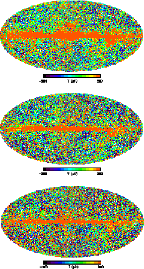
Figure 1: From top to bottom, combined Q-, V-, and W-band radiometer maps created by making maps for each individual radiometer and summing them using the weighting scheme of equation (24) of Hinshaw II.

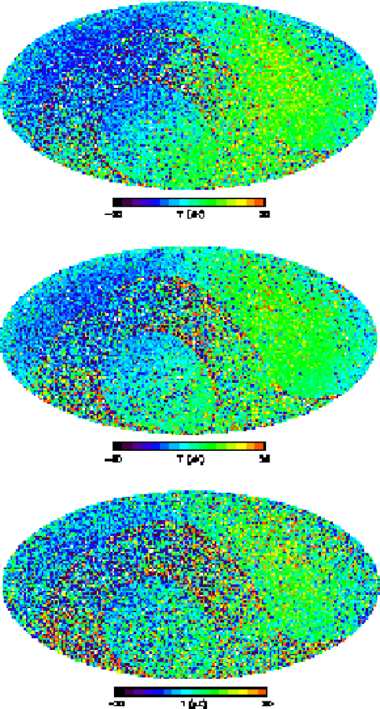
Figure 2: From top to bottom, combined Q-, V-, and W-band radiometer difference maps (${\Delta}T_{\rm WMAP}-{\Delta}T$) created with combined WMAP maps and the maps shown in Figure 1. There are two structures present in these data: a speckled pattern related to the statistical weighting of first day data; and a dipolar structure of amplitude $\approx$ 7 $\mu$K in the direction $(l_{\rm gal},b_{\rm gal})\approx$ ($-$86^∘,$-$19^∘). See also Figure 4.

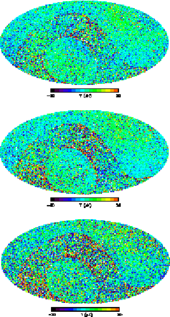
Figure 3: Same as Figure 2, but with the residual dipolar structure removed. The remaining structure is due to our including the second-order term when computing the Doppler shift of the monopole; the WMAP team does not include this term in their calculations. See also Figure 4.

Figure 4: Difference histograms ${\Delta}T_{\rm WMAP}-{\Delta}T$ for the Q-, V-, and W-band data. The solid line is a histogram of the data shown in Figure 2, while the dashed line corresponds to Figure 3.

3 Determination of Asymmetry in Generated Maps

To determine asymmetry in summed power between arbitrarily defined opposite hemispheres, we follow Eriksen I and Hansen I by principally analyzing a combined map consisting of foreground-corrected V- and W-band maps. We perform foreground corrections using the method of Bennett et al. (2003b; hereafter Bennett II), and combine the maps using equation (24) of Hinshaw II. To compute cut-sky pseudo-$C_{l}$ power spectra, we implement the Master algorithm of Hivon et al. (2002), summarized in Appendix A of Hinshaw II. This differs from Eriksen I and Hansen I, who use the maximum likelihood method of Hansen et al. (2002) and Hansen & Górski (2003) to compute cut-sky power spectra. As discussed in §2.2 of Efstathiou (2004), use of the Hivon et al. method is not optimal in that there is a estimator-induced variance that makes it an inaccurate determiner of power in the low-$l$ regime, with the variance of the sampling distribution increasing with mask size. In this particular work, however, the use of the Hivon et al. method does not have a detrimental effect in that we are not interested in power amplitudes or the magnitudes of the ratio per se, but rather in how the observed ratios compare with sampling distributions that are determined via simulations and thus have the estimator-induced variance built in.

To compute asymmetry as a function of location on the sky, we define 101 independent NP orientations on the northern galactic hemisphere ($l_{\rm gal}$ = [0^∘,324^∘] with ${\Delta}l_{\rm gal}$ = 36^∘ and $b_{\rm gal}$ = [0^∘,90^∘] with ${\Delta}b_{\rm gal}$ = 9^∘; $l_{\rm gal}$ is not defined for $b_{\rm gal}$ = 90.0^∘). We apply two Kp2+hemispherical masks for each NP orientation and compute power spectra for the northern and southern hemispheres for $l\leq$ 64. We then calculate asymmetry over arbitrary multipole ranges, using arbitrary weightings (e.g., $w_{l}$ = 1, or $w_{l}~{}=~{}l(l+1)$), via:

$$A_{\rm obs}(l_{\rm gal},b_{\rm gal},l_{\rm min},l_{\rm max},w_{l})~{}=~{}\frac{\sum_{l_{\rm min}}^{l_{\rm max}}w_{l}C_{l}^{\rm NH}}{\sum_{l_{\rm min}}^{l_{\rm max}}w_{l}C_{l}^{\rm SH}}\,.$$ (6)

(In this work, we assume $w_{l}~{}=~{}l(l+1)$.) We examine each direction separately because of the number of pixels within the north and south masks is generally unequal; this causes the expected mean asymmetry value derived from simulations to differ from unity and to vary as a function of direction.

We compare our results with simulated sampling distributions. We use the HEALPix facility synfast to generate random universes by sampling from a given power spectrum. Current theoretical bias leads us to adopt the LCDM power spectrum derived from a running-index primordial spectrum using WMAP, CBI, and ACBAR data (which we denote RI (catalog ADS/Sa.WMAP#lcdm_ri_model_yr1_v1.txt)). We simulate 512 random universes, generating two copies of each. We convolve the two copies with the 21$\arcmin$ V-band and 13$\arcmin$ W-band beam responses respectively. From the two band-specific maps, we generate six noisy radiometer-specific maps, where we assume Gaussian pixel noise $\sim N(0,\sigma_{o}/\sqrt{n_{{\rm obs},p}})$ and use tabulated radiometer-specific values of $\sigma_{o}$. We co-add and analyze the six noisy simulation maps in the manner of our six observed maps, generating a distribution of 512 asymmetry values in each defined direction $(l_{\rm gal},b_{\rm gal})$.

We observe that the sampling distribution for $A(l_{\rm gal},b_{\rm gal})$, the ratio of two Gaussian-distributed random variables under the null hypothesis, is approximately lognormal:

$$A_{\rm obs}(l_{\rm gal},b_{\rm gal})~{}\sim~{}f(A,\mu,\sigma)~{}=~{}\frac{1}{\sqrt{2\pi}(A-\mu)\sigma}\exp\left[-\left(\frac{\ln(A-\mu)}{\sqrt{2}\sigma}\right)^{2}\right]\,.$$ (7)

This is expected because if, for instance, the distribution mean is unity, one would expect the same probability for observing asymmetry values of, e.g., 0.5 and 2.0. We fit lognormal distributions to the data to estimate significances (see Figure 5); otherwise, estimates would be limited to values $\alpha\gtrsim 1/512\sim 10^{-3}$ and would be inaccurate in the distribution tails. For a given set of parameters $(l_{\rm gal},b_{\rm gal},l_{\rm min},l_{\rm max})$, we sum over the multipole range, obtain best-fit values $\mu_{o}$ and $\sigma_{o}$ by maximizing the sum of the log-likelihoods for each datum, and determine what we call the directional significance, $\alpha_{\rm dir}$:

$$\alpha_{\rm dir}~{}=~{}{\rm min}[\int_{0}^{A_{\rm obs}}dAf(A,\mu_{o},\sigma_{o})~{},~{}\int_{A_{\rm obs}}^{\infty}dAf(A,\mu_{o},\sigma_{o})]\,.$$ (8)

$\alpha_{\rm dir}$ is an estimate of the probability that a random Gaussian field exhibits at least as much power asymmetry as observed in the data in the specific direction $(l_{\rm gal},b_{\rm gal})$.

While the directional significance is useful for, e.g., visualization, it is not sufficient to establish the global significance of asymmetry for a given dataset, $\alpha_{\rm global}$, which is an estimate of the probability that the random Gaussian field exhibits at least as much asymmetry as observed in the data in any direction. We cannot easily obtain $\alpha_{\rm global}$ because the directional distributions are correlated, with the degree of correlation dependent on the multipole range considered. (We observe that because the distributions are correlated, the simplest Bonferroni correction$-$multiplying the smallest observed value of directional significance, $\alpha_{\rm dir,min}^{\rm obs}$, by the number of examined directions, 101$-$is too conservative.) A rigorous approach would involve transforming our simulation results to log-space and numerically determining the correlations between all combinations of grid points, which would allow us to specify the 101-dimensional Gaussian probability function. We would then examine this function using methods described in, e.g., Adler (2000) to estimate $\alpha_{\rm global}$. However, as this calculation is very computationally intensive, we adopt a simpler approach: we compare $\log(\alpha_{\rm dir,min}^{\rm obs})$ with its probability distribution, which we find to be approximately an extreme-value distribution:

$$\log(\alpha_{\rm dir,min}^{\rm obs})~{}\sim~{}g[\log(\alpha_{\rm dir,min})]~{}=~{}\frac{1}{\sigma}\exp\left[\frac{\mu-\log(\alpha_{\rm dir,min})}{\sigma}-\exp\left(\frac{\mu-\log(\alpha_{\rm dir,min})}{\sigma}\right)\right]\,.$$ (9)

As this distribution is the limiting distribution for the largest element of a set of independent samples from a normal distribution, this finding is not unexpected. In a similar manner to that described above, we determine best-fit values $\mu_{o}$ and $\sigma_{o}$ (see Figure 5); the estimated global significance is then:

$$\alpha_{\rm global}~{}=~{}1-\exp\left[-\exp\left(\frac{\mu_{o}-\log(\alpha_{\rm dir,min}^{\rm obs})}{\sigma_{o}}\right)\right]\,.$$ (10)

We consider $\alpha_{\rm global}\leq$ 0.05 to be significant. We make no claim that this computation is the optimal proxy for a full Gaussian random field calculation; more accurate and/or powerful, yet still computationally simple, hypothesis tests may exist.

Figure 5: Example fit of a lognormal distribution to 512 simulated asymmetry values for given direction $(l_{\rm gal},b_{\rm gal})$, which is used to estimate $\alpha_{\rm dir}$ (top panel; see equation 8), and example fit of an extreme-value distribution to 512 simulated values of $\alpha_{\rm dir,min}$, which is used to estimate $\alpha_{\rm global}$ (bottom panel; see equation 10).

In Figure 6 we show the direction of maximum significance and $\alpha_{\rm global}$ for the multipole range $l$ = [2,$l_{\rm max}$]. Unlike Hansen I, who find that the direction of maximum significance is always toward the galactic NP if $l_{\rm min}$ = 2, we find that it moves from the vicinity of the galactic NP toward the galactic plane as $l_{\rm max}$ increases. For instance, for the range $l$ = [2,40], we observe that $\alpha_{\rm dir}^{\rm plane}\sim 10^{-3}\alpha_{\rm dir}^{\rm NP}$. For $l_{\rm min}\geq$ 5, we find results consistent with those of Hansen I. Over the full multipole range that we consider, $l$ = [2,64], we find a maximum directional significance $\alpha_{\rm dir}$ = 3.3$\times$10^-6 in the direction $(l_{\rm gal},b_{\rm gal})$ = (72^∘,9^∘), with global significance $\alpha_{\rm global}$ = 2.6$\times$10^-4. (This is consistent with the $\sim$ 10^-3 value determined by Hansen I using 2048 simulations, without fits of sampling distributions.) This result indicates clearly that there is power asymmetry in the WMAP data.

Figure 6: Direction of maximum asymmetry in galactic coordinates (top two panels), and the global significance $\alpha_{\rm global}$ (bottom panel), computed in bins $l$ = [2,$l_{\rm max}$] for the RI input power spectrum. The horizontal dotted line in the top two panels indicates the position of the ecliptic NP, while the dot-dashed line in the bottom panel marks $\alpha_{\rm global}$ = 0.05.

At what scales is power asymmetry most evident? Mindful that there could be a number of causes manifesting themselves at different scales, we determine the smallest ranges with significant asymmetry. We compute $\alpha_{\rm global}$ in multipole bins with minimum width ${\Delta}l$ = 2. (We do not examine each multipole singly because the computation of $\alpha_{\rm global}$ is complicated at low $l$ by the fact that the sampling distributions for $C_{l}$ are truncated at zero, resulting in a considerable number of asymmetry values that are either zero or infinite. This is not an issue for ${\Delta}l\geq$ 2.) We start with ${\Delta}l$ = 2, and increase the bin size until no more significant bins are found. For a given ${\Delta}l$, we examine all bins (e.g., for ${\Delta}l$ = 2, we examine $l$ = [2,3], then [3,4], etc.), and mark those for which $\alpha_{\rm global}\leq$ 0.05. If two or more significant bins overlap, we mark only the most significant bin. For each ${\Delta}l$, we examine only those multipoles that have not yet been marked as part of a significant bin (e.g., if we find that only the bin $l$ = [2,3] is significant for ${\Delta}l$ = 2, the first bin we would examine for ${\Delta}l$ = 3 is [4,6], and not [2,4]). We note that this binning algorithm is not meant as a rigorous statistical exercise (we examine so many bin combinations that a number of of the chosen bins may be false positives) but rather as a guide to further examination of the data. In Figure 7 we show the result: we find twelve significant ranges, including two pairs and one triplet of (nearly) contiguous bins (separated by at most one bin). The gaps between significant bins are treated as single, insignificant bins for purposes of plotting. As shown in the bottom panel of Figure 7, combining (nearly) contiguous bins does not necessarily yield a more significant result. The large number of significant bins and the fact that we discern no general trend in the direction of $A_{\rm obs}^{\rm max}$ lead us to conclude that the process(es) contributing to the observed asymmetry (e.g., residual foreground emission) are spatially complex.

The bins $l$ = [2,3] and $l$ = [6,7] appear anomalously significant, with $\alpha_{\rm global}~{}\lesssim$ 10^-6 (the value depends very sensitively upon the fit parameters of the extreme-value distribution and we cannot determine it accurately). For $l$ = [2,3], the direction of maximum significance is ($l_{\rm gal},b_{\rm gal}$) = (144^∘,9^∘), with $C_{2,3}^{N}$ = {9.7,1.1} and $C_{2,3}^{S}$ = {301.7,755.9}, while for $l$ = [6,7], the corresponding values are ($l_{\rm gal},b_{\rm gal}$) = (180^∘,27^∘), $C_{6,7}^{N}$ = {303.6,196.7}, and $C_{6,7}^{S}$ = {51.7,0.0}. We confirm that the simulated values of $\alpha_{\rm global}$ in each case follow extreme-value distributions with no discernible deviation that may affect the estimation of significance. Thus we take the observed significances at face value and conclude that there is highly significant power asymmetry at the largest scales. We note that we determine the direction of maximum asymmetry for $l$ = [2,3] to be in the galactic plane, while for Hansen I it is the galactic NP (for $l$ = [2,4]; we confirm that our result does not change if we include $l$ = 4).

To determine the sensitivity of $\alpha_{\rm global}$ to changes in frequency, we simulate separate sets of co-added Q-, V-, and W-band data, as well as a set of co-added data from all three bands. In all cases, we find results that are similar, both qualitatively and quantitatively, to those presented above; for instance, over the multipole range $l$ = [2,64], we find $\alpha_{\rm global}$ = 3.0$\times$10^-4 (Q), 6.2$\times$10^-4 (V), 7.1$\times$10^-4 (W), and 2.3$\times$10^-4 (all bands). This finding is consistent with that of Hansen I, who analyze Q-band data with a Kp0 mask and find persistent asymmetry.

We also repeat our analysis using four alternate theoretical and phenomenological power spectra as input to simulations:

1. a running-index spectrum similar to the RI spectrum, with 2dF and Lyman-$\alpha$ data also included in the computation (BF (catalog ADS/Sa.WMAP#lcdm_bf_model_yr1_v1.txt));

2. the theoretical LCDM power spectrum derived from a power-law primordial spectrum (PL (catalog ADS/Sa.WMAP#lcdm_pl_model_yr1_v1.txt));

3. the observed WMAP “One-Year Combined TT Power Spectrum” (TT (catalog ADS/Sa.WMAP#comb_tt_powspec_yr1_v1p1.txt));

4. and the same as immediately above, but optimally smoothed via local linear smoothing, with bandwidth chosen by leave-one-out cross-validation (see, e.g., Fan & Gijbels 1996; OP).

For each spectrum, we compute $\alpha_{\rm global}$ within the previously defined RI bins, as opposed to defining a new set of bins. This has little effect on our results, which we display in Figure 8. We find that $\alpha_{\rm global}$ is largely insensitive to the choice of power spectrum; while the variance of the distribution of simulated asymmetry values differs for each, the differences are insufficient to qualitatively affect results. However, we do note that the range $l$ = [49,51], significant given the RI spectrum, is not significant for any other spectrum.

In Figures 9a-3, we display contours of $\alpha_{\rm dir}$ for each of the twelve globally significant multipole ranges shown in Figure 7. The direction and significance of maximum asymmetry in each panel in these figures maps directly back to the values plotted in the top three panels of Figure 7. Interestingly, these contours exhibit evidence of a relationship between the ecliptic plane and both the direction of maximum significance and the contours of least significance ($\alpha_{\rm dir}\approx$ 0.2-0.5). We find that in four of the twelve plots, the direction of maximum asymmetry lies within $\approx$ 4^∘ of the ecliptic plane and in eight of twelve, within $\approx$ 20^∘. The coarseness of our coordinate grid precludes an exact quantitative interpretation, but we note that the probability of sampling a point within 4^∘ of the ecliptic plane is 0.07, and within 20^∘, 0.34; the probability of what we observe is $p_{\rm binomial}\lesssim$ 0.01 in both cases.

We also observe that, for large scales, the contours of least significance appear to follow great circles; furthermore, the great circle for $l$ = [6,7] passes over the ecliptic poles. (Great circle-like structures appear at other scales as well, but not as strikingly.) While the significance of such an alignment of contours is difficult to quantify, we visually examine contour plots created from simulated datasets and find no discernible trend toward the formation of great circles. In Figure 10, we concentrate on the lowest four multipole ranges shown in Figure 8. The dotted and dash-dotted lines in these figures represent great circles inclined relative to the ecliptic and galactic planes, respectively. Note that we place the lines by eye and make a purely qualitative comparison of goodness-of-fit. For $l$ = [2,3] and $l$ = [6,7], great circles defined in ecliptic coordinates with inclinations $\approx$ 30^∘ and $\approx$ 90^∘ respectively appear to fit the contours of least significance better than their galactic coordinate counterparts; for $l$ = [8,10] and [11,14], there is no clear preference for either coordinate system. In Figure 11, we demonstrate that the contours and great circles for $l$ = [2,3] are frequency independent: they are observed within each radiometer band separately, with the results in each band relying on completely independent sets of simulations. We conclude that whatever causes power asymmetry at the largest scales may be related to the ecliptic, but at the same time the underlying process is frequency independent.

In Figure 12, we show the relationship between the great circle for the $l$ = [2,3] and the axes defined by de Oliveira-Costa et al. that maximize the angular momentum dispersion of the quadrupole and octopole in their wave-function paradigm, as well as the four normals to the planes defined by the multipole vectors of Schwarz et al. All except the ${\bf w}^{(3,3,1)}$ vector of Schwarz et al. point in the same general direction (the “axis of evil,” as dubbed by Land & Magueijo 2005a), near a contour of minimum significance ($\alpha_{\rm dir}>$ 0.4). However, they also point near the CMB dipole. In the next section, we examine the effect of changing the magnitude of the velocity of the CMB dipole on observed asymmetry.

Figure 7: Direction of maximum asymmetry in galactic coordinates (top two panels), the corresponding significance $\alpha_{\rm dir}$ (third panel), and the global significance $\alpha_{\rm global}$ (bottom panel), as a function of $l$, for the RI input power spectrum. See §3 for a description of how bin widths are determined. The horizontal dotted line in the top two panels indicates the position of the ecliptic NP, while the dot-dashed line in the bottom panel marks $\alpha_{\rm global}$ = 0.05. The additional dotted lines in the bottom panel indicate the values of $\alpha_{\rm global}$ if we combine (nearly) contiguous significant ranges: $l$ = [6,10], [6,14], [8,14], [22,25], and [43,51].

Figure 8: Similar to the bottom panel of Figure 7, showing global significance $\alpha_{\rm global}$ as a function of $l$ for the five different input power spectra listed in the text. The top panel of this figure is the same as the bottom panel of Figure 7. This figure demonstrates that $\alpha_{\rm global}$ is relatively insensitive to the choice of power spectrum.

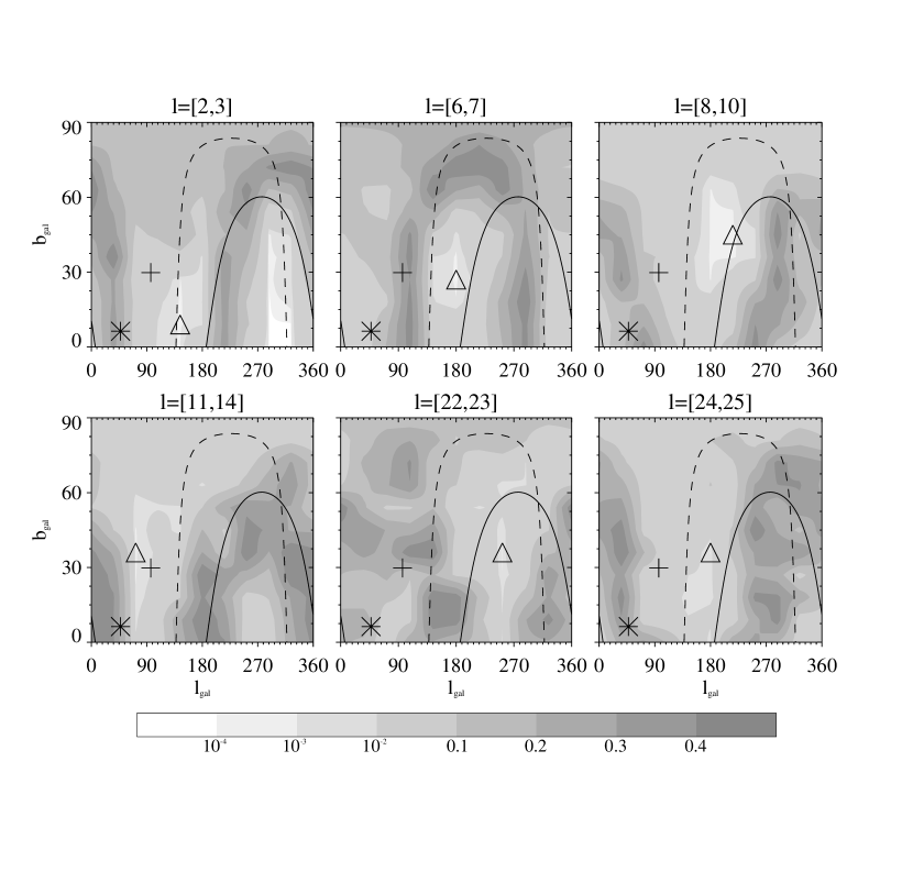
Figure 9a: Directional significance contour plots showing the significance of observed asymmetry as a function of NP location in $(l_{\rm gal},b_{\rm gal})$ within multipole bins in which the global significance of asymmetry is $\alpha\leq$ 0.05. The minimum bin width is ${\Delta}l$ = 2. The direction of maximum significance is labeled with a triangle, the cross and solid line indicate the ecliptic NP and plane respectively, and the asterisk and the dashed line indicate the supergalactic NP and plane respectively.

Fig. 9b.

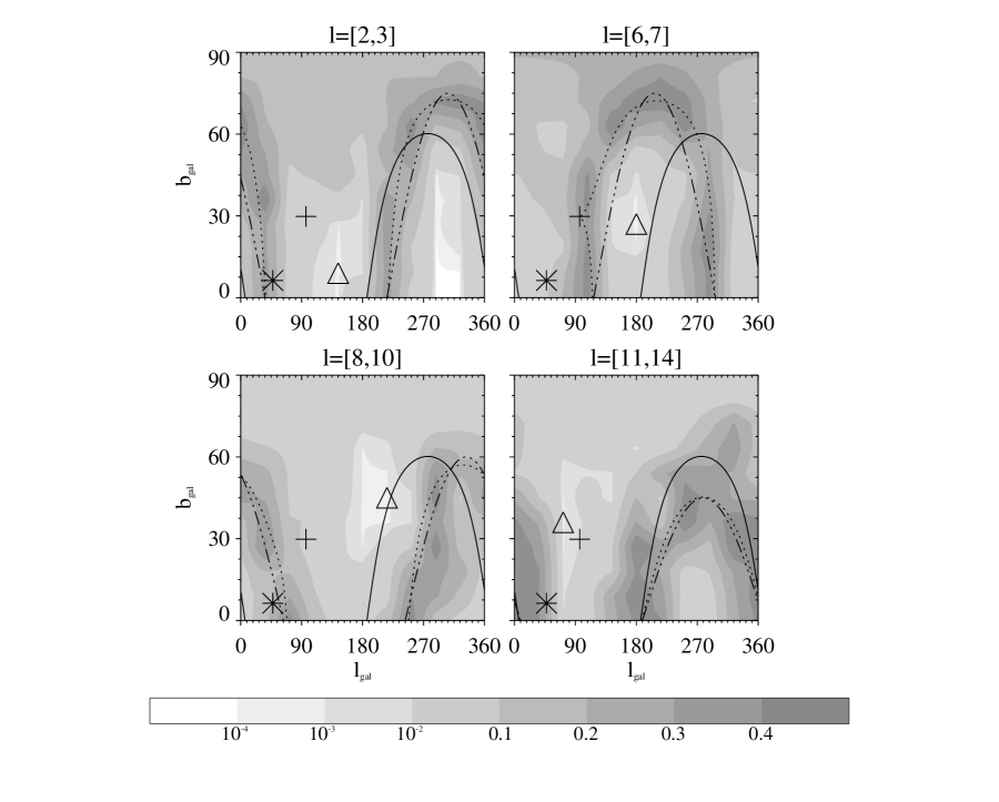
Figure 10: Directional significance contour plots for the lowest four multipole bins shown in Figure 9a (see this figure for an explanation of symbols). All four plots exhibit contours of least significance that appear to follow great circles. The dotted and dash-dotted lines represent great circles inclined relative to the ecliptic and galactic planes, respectively. The lines are illustrative and their placement is done by eye.

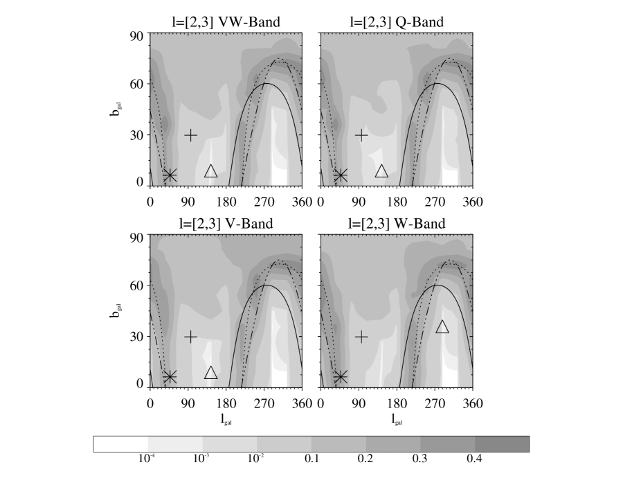
Figure 11: Same as the upper left panel of Figure 10, with co-added Q-, V-, and W-band data displayed in the upper right, lower left, and lower right panels respectively. See Figures 9a and 10 for explanations of symbols. We conclude that the process causing power asymmetry at the largest scales is insensitive to frequency.

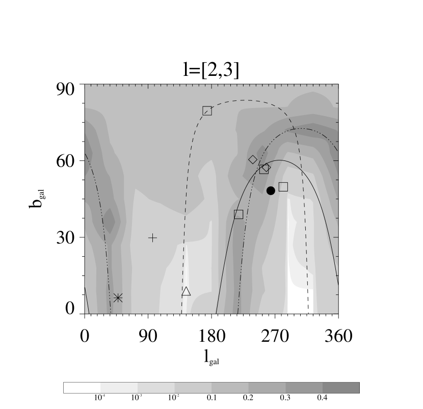
Figure 12: Upper left panel of Figure 10 with the great circle in galactic coordinates removed. The diamonds represent the pointing direction of the quadrupole (lower right) and octopole (upper left) preferred axes defined by de Oliveira-Costa et al., while the squares represent the pointing direction of normals to the planes defined by multipole vectors derived by Schwarz et al. The filled circle shows the direction of the CMB dipole.

4 Effect of Map-Making Algorithmic Assumptions Upon Observed Asymmetry

A heretofore unexamined aspect of the asymmetry issue is the effect of altering the map-making algorithm. For instance, what if maps were made using no foreground mask at all, or a reduced mask, rather than the Kp8 mask with no edge smoothing? Because of the elliptical beam response, maps would be affected by propagated echoes of bright Galactic sources, as noted by Hinshaw I. But would these echoes have any discernible effect on the observed asymmetry? (We realize that in this example using no foreground mask at all is clearly a wrong step no one would make; our goal in these tests is simply to establish how sensitive asymmetry is to changes in the map-making algorithm.)

The alterable aspects of our map-making algorithm, both major and minor, fall into a number of categories:

1. The mapping paradigm, involving issues which are too complex to address in the current work:

   • The assumption of Gaussian pixel noise and its subsequent use in least-squares estimates.

   • The assumption that the matrix product (${\bf M}^{\rm T}{\bf M})^{-1}$ is diagonally dominant and is $\approx{\vec{n}}_{\rm obs}^{-1}$. This goes hand-in-hand with the assumption that the radiometers have $\delta$-function spatial response, an assumption which we expect has little to no effect in the low-$l$ regime.

2. Aspects which are currently not alterable given the data we have:

   • The algorithm by which the raw data are calibrated (Hinshaw I, §2.2).

   • The assumption of equal statistical weights for each datum.

3. Aspects which we directly examine:

   • The assumption that $T_{\rm o}$ = 2.725 K.

   • The assumption that the Sun’s velocity relative to the CMB is $(v_{\odot,\rm gal}^{x},v_{\odot,\rm gal}^{y},v_{\odot,\rm gal}^{z})$ =
     ($-$26.26,$-$243.71,274.63) km s^-1 (or $v_{\odot,\rm gal}$ = 368.11 km s^-1).

   • The effect of including the loss-imbalance parameters (Table 3 of Jarosik et al.).

   • The use of the Kp8 galactic mask without edge smoothing.

   • The use of Lagrange interpolating polynomials to determine radiometer normal vectors as a function of time.

   • The assumption that the planetary cut is $\theta_{\rm cut}$ = 1.5^∘.

   • A step beyond map-making: the use of the same foreground maps, in the same proportion, as the WMAP team (Bennett II, §6).

We also examine the sensitivity of asymmetry to temperature map zero points, which the WMAP team derives by fitting a phenomenological model to southern galactic hemisphere data (Bennett II, §5). Normally, changing the zero point, i.e., changing the monopole component of the anisotropy map, should have no effect on higher multipoles. However, power leakage from the monopole in, e.g., the Master algorithm means that any uncertainty in the zero point can in theory affect measurements of asymmetry. The average temperatures in the V-band and W-band maps are $\approx$ 78 $\mu$K and 75 $\mu$K, respectively, with variance $\sim$ 1 $\mu$K. We confirm that changing the zero point by amounts up to 10 $\mu$K has negligible impact upon $\alpha_{\rm global}$.

After altering the value of a given parameter (while holding the other parameter values to their default values), we create new V- and W-band radiometer maps. We combine these maps into a new co-added map that we analyze using the methods described in §3. To determine if altering mapping parameters can reduce or eliminate all asymmetry, we concentrate upon the range $l$ = [2,64] (Table 1); however, we also examine the range $l$ = [2,3] to gauge the effect of changes on large-scale asymmetry.

Table 1: Effect of Changing Mapping Parameters on Power Asymmetry for l = [2,64]

Changed Parameter	$\alpha_{\rm dir}$ Quartiles	$\alpha_{\rm dir,min}$	$(l_{\rm gal},b_{\rm gal})$	$\alpha_{\rm global}$
Default Map	(0.152,0.0132,2.56$\times$10-3)	3.30$\times$10-6	(72∘,9∘)	2.55$\times$10-4
No First Day Data	(0.152,0.0132,2.58$\times$10-3)	3.30$\times$10-6	(72∘,9∘)	2.55$\times$10-4
To = 2.724 K ($-$1$\sigma$)	(0.147,0.013,2.58$\times$10-3)	3.30$\times$10-6	(72∘,9∘)	2.55$\times$10-4
To = 2.726 K (+1$\sigma$)	(0.152,0.013,2.58$\times$10-3)	3.30$\times$10-6	(72∘,9∘)	2.55$\times$10-4
Vd = 366.24 km s-1 ($-$1$\sigma$)	(0.144,0.013,2.26$\times$10-3)	4.59$\times$10-6	(72∘,9∘)	3.46$\times$10-4
Vd = 369.98 km s-1 (+1$\sigma$)	(0.147,0.014,2.75$\times$10-3)	2.35$\times$10-6	(72∘,9∘)	1.88$\times$10-4
Vd = 371.85 km s-1 (+2$\sigma$)	(0.157,0.017,3.77$\times$10-3)	2.10$\times$10-6	(72∘,9∘)	1.69$\times$10-4
Vd = 373.72 km s-1 (+3$\sigma$)	(0.147,0.024,5.07$\times$10-3)	2.63$\times$10-6	(72∘,9∘)	2.08$\times$10-4
No Mask	(0.148,0.013,2.86$\times$10-3)	4.11$\times$10-6	(72∘,9∘)	3.13$\times$10-4
No Interpolation	(0.093,7.20$\times$10-3,4.39$\times$10-4)	5.70$\times$10-8	(72∘,9∘)	6.20$\times$10-6
Linear Interpolation	(0.152,0.0132,2.58$\times$10-3)	3.30$\times$10-6	(72∘,9∘)	2.55$\times$10-4
Planet Cut: $\theta_{\rm cut}$ = 0.0∘	(1.45$\times$10-7,5.77$\times$10-14,2.17$\times$10-19)	1.40$\times$10-26	(72∘,9∘)	0.0
Planet Cut: $\theta_{\rm cut}$ = 0.5∘	(0.147,0.0154,2.28$\times$10-3)	2.63$\times$10-6	(72∘,9∘)	2.08$\times$10-4

Monopole Temperature.

We find that altering the monopole temperature by 1$\sigma$ (0.001 K) has little effect on the distribution of significances, and none on $\alpha_{\rm global}$.

Dipole Velocity Magnitude.

We test changing the magnitude of the dipole velocity along the direction ($l_{\rm gal}$,$b_{\rm gal}$) = (263.85^∘,48.25^∘). (Testing changes on a grid of dipole locations is currently too computationally intensive.) We find that positive changes $\gtrsim$ 1$\sigma$ ($\gtrsim$ 2 km s^-1) can have a marked effect upon $\alpha_{\rm global}$ at the largest scales, even sometimes rendering asymmetry insignificant (Figure 13). At smaller scales, the effect on asymmetry is minimal (e.g., bottom panels of Figure 13). Note that the velocities that we assume in map-making do not match that used to calibrate the data (the COBE DMR dipole), so we cannot state with certainty that changing the dipole velocity can by itself eliminate asymmetry at the largest scales.

To determine the effect of using the Master algorithm upon quadrupole power, we examine both uncorrected and corrected cut-sky power spectrum estimates. As illustrated in Figure 14, the uncorrected Kp2+hemisphere cut-sky power spectrum estimates for the quadrupole (triangles and boxes for the north and south hemispheres respectively in the middle panel) are greatly affected when we increase the dipole velocity, with the ratio of estimates tending toward unity (thus reducing the significance of asymmetry). The subsequent shifting of dipole power to the quadrupole via mode coupling in the Master algorithm changes the quadrupole power by $\lesssim$ 10% (varying slightly as a function of direction). We conclude that the observed reduction in the significance of asymmetry is primarily due to increased quadrupole power in each hemisphere, and is not purely an artifact of the Master algorithm.

It is important to note that increasing the sky coverage reduces the effect of dipole velocity upon quadrupole power, and if we use the Kp2 mask alone, the effect is minimal (circles, middle panel). Thus changing the dipole velocity has negligible impact on “full sky” power spectra, and does not help to explain any supposed irregularities in these spectra (see, e.g., Land & Magueijo 2005b and Vale 2005). It is also important to note that the increase in the dipole power for the Kp2 cut sky at $\gtrsim$ 1$\sigma$ (top panel, Figure 14) does not necessarily rule out higher velocities, as the offsets of the tested velocity from the true velocity and from the COBE DMR velocity will have a non-negligible effect on the dipole power estimate, and the contribution of the primordial dipole component is unknown but could be significant ($\sim$ 1000 $\mu$K).

In Figure 15, we display how the contours of directional significance evolve as the magnitude of the dipole velocity increases. In addition to an increase in $\alpha_{\rm global}$, we observe that the direction of maximum significance migrates toward the ecliptic plane, with the great circle still evident, though not as strongly, at 3$\sigma$.

Figure 13: Plots of $\alpha_{\rm global}$ as a function of shifted dipole velocity (1$\sigma$ = 1.87 km s^-1), for the multipole ranges displayed in each panel. The dot-dashed line in each panel represents $\alpha_{\rm global}$ = 0.05. This figure illustrates that changing the dipole velocity can have a marked effect upon the significance of asymmetry at the largest scales. However, since the dipole velocities used to generate this figure differ from the dipole velocity used to calibrate the data, the uncertainty of each datum is unknown.

Figure 14: Uncorrected Kp2 cut-sky power (circles) and uncorrected Kp2+hemisphere cut-sky power (triangles and boxes for north and south respectively) for the dipole (top), quadrupole (middle), and octopole (bottom), as a function of change in the magnitude of the dipole velocity (1$\sigma$ = 1.87 km s^-1). The assumed NP is the galactic NP. This figure shows that changing the dipole velocity acts to increase the Kp2+hemisphere cut-sky power for the quadrupole, so that asymmetry approaches unity and becomes insignificant. It also demonstrates that for the Kp2 cut-sky, the effect of shifting the velocity is concentrated at the dipole, as expected.

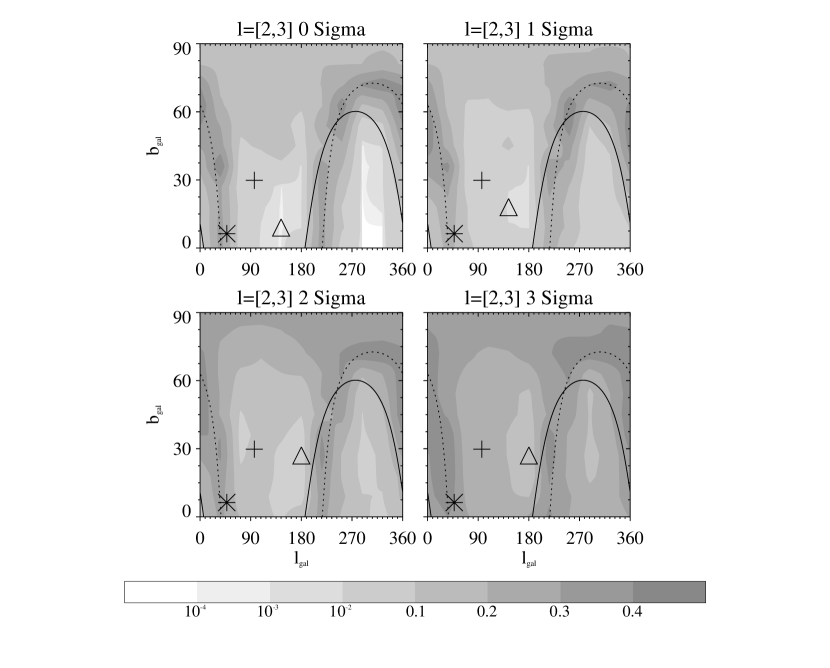
Figure 15: Same as the upper left panel of Figure 10, with the magnitude of the dipole velocity increased by 1$\sigma$ (= 1.87 km s^-1), 2$\sigma$, and 3$\sigma$ (upper right, lower left, and lower right, respectively). The effects of increasing the dipole velocity are to make $\alpha_{\rm global}$ insignificant, to make the direction of maximum significance migrate toward the ecliptic plane, and to make the apparent great circle less visually striking.

Loss Imbalance.

We set $x_{\rm im}$ in eqs. (3) and (5) to zero. This has no discernible effect on asymmetry.

Masking.

To gauge the effect of masking, we make maps with no mask at all. This has virtually no effect on asymmetry, presumably because the scale size of the aforementioned galactic echoes is smaller than those probed in our analysis.

Interpolation to Determine Spacecraft Orientation.

The quaternions that encode spacecraft orientation are recorded at the beginning of each 1.536 s science frame, while data are sampled up to 30 times per frame. Interpolation is normally done using Lagrange interpolating polynomials (see the Appendix for details). We test the effect of making maps with no interpolation and with linear interpolation. Turning off interpolation leads to pointing errors on the order of degrees, and asymmetry becomes more pronounced, with the significance increasing by two orders of magnitude ($\alpha_{\rm global}\sim$ 10^-6 for $l$ = [2,64]). The use of linear interpolation has virtually no effect on asymmetry. This indicates that the WMAP team’s use of Lagrange interpolating polynomials is a conservative algorithmic choice, and that the small errors in the recorded orientation of the spacecraft and the determination of instrumental boresights ($\lesssim$ 1$\arcmin$; see §3.3.1 and 3.3.2 of Hinshaw I) have little to no effect on asymmetry.

Planetary Cut.

If a planet is determined to be within $\theta_{\rm cut}$ = 1.5^∘ of either radiometer’s normal vector, the temperature map is not updated for either. This value is conservative, being over four times the FWHM of the V-band radiometer beam size (this helps mitigate the effect of non-Gaussian shoulders in the beam profile). We test the effects of making maps assuming $\theta_{\rm cut}$ = 0.5^∘, and $\theta_{\rm cut}$ = 0.0^∘. In both cases, asymmetry becomes more pronounced over the full range $l$ = [2,64]. If $\theta_{\rm cut}$ = 0.5^∘, the effect upon significances is $\lesssim$ 10%, while if $\theta_{\rm cut}$ = 0.0^∘, $\alpha_{\rm global}\rightarrow$ 0. The former result indicates that reasonably changing $\theta_{\rm cut}$ would have virtually no effect on asymmetry.

Foreground Maps.

We test the effect of foreground corrections by changing the relative normalizations of the three foreground maps (dust, H_α, and synchrotron; see Bennett II for details). We find that small shifts ($\sim$ 10%) have little to no effect upon asymmetry, which is not unexpected because of the markedly reduced level of foreground emission outside the Kp2 mask with respect to that in the galactic plane. (Because of the large number of normalization combinations tested, we do not display our results in Table 1.) To have a discernible effect, order-of-magnitude changes in the normalizations are required. This demonstrates that asymmetry is not simply related to uncertainties in relative normalization.

5 Summary and Conclusions

In this work, we analyze first-year WMAP data to determine the significance of asymmetry in summed power between opposite arbitrarily defined hemispheres. We perform this analysis on maps that we compute directly from the calibrated time-ordered data, using a map-making algorithm that we have developed to be similar to that used by the WMAP team. By creating our own maps, we are able to determine whether altering elements of the map-making algorithm is sufficient to affect the observed asymmetry (and perhaps to render it statistically insignificant).

We follow Eriksen I and Hansen I by analyzing co-added V- and W-band foreground corrected maps, and like these groups we find that there is a significant difference in summed power between arbitrarily defined northern and southern hemispheres. We compute significance by simulating data from the running-index LCDM power spectrum, determining the most significant deviation from expectation in each dataset, fitting an extreme-value distribution to these deviations, and computing the tail integral of the best-fit distribution. Over the multipole range $l$ = [2,64], we estimate the global significance of asymmetry to be $\alpha_{\rm global}\sim$ 10^-4, and we find that this value is not sensitive either to frequency (as determined by examining co-added data in the Q, V, and W bands, and within each radiometer alone), or to the details of the power spectrum used as input to simulations. These results clearly indicate that the posited power asymmetry in WMAP data is real. We determine the smallest multipole ranges for which $\alpha_{\rm global}\leq$ 0.05; we find twelve such ranges, including $l$ = [2,3] and [6,7], for which $\alpha_{\rm global}\rightarrow$ 0. Contour plots made for these ranges indicates an association between the direction of maximum asymmetry and the ecliptic plane (four of twelve directions within $\approx$ 4^∘ and eight within $\approx$ 20^∘; $p_{\rm binomial}\lesssim$ 0.01), although one must be mindful of the coarseness of our coordinate grid. At large scales, the contours of least significance ($\alpha_{\rm dir}\approx$ 0.2-0.5) may be fit by eye with great circles inclined relative to the ecliptic plane, with inclinations of $\approx$ 30^∘ and 90^∘ for $l$ = [2,3] and [6,7] respectively. We find that the $l$ = [2,3] great circle is insensitive to frequency and that it passes over preferred quadrupole and octopole axes derived by de Oliveira-Costa et al. and Schwarz et al., as well as the pointing direction of the CMB dipole.

We test the robustness of our results by using examining the effect of map-making algorithmic assumptions upon asymmetry. We create and analyze new maps after changing the monopole temperature, the magnitude of the dipole velocity, the masks, the method of interpolation used to determine the pointing direction of radiometer normal vectors as a function of time, the planetary cut, and the relative normalizations of the foreground maps. In virtually all cases, the alterations had little to no effect upon asymmetry either for the range $l$ = [2,64] or at the largest scales. An exception to this is the magnitude of the dipole velocity: we find that increasing it has a marked effect on the direct (i.e., uncorrected) estimate of quadrupole power in the Kp2+hemisphere cut skies, increasing power in both the northern and southern hemispheres such that asymmetry approaches unity (and becomes insignificant). Changing the magnitude of the dipole velocity is a frequency-independent change, consistent with observations that the significance of asymmetry is frequency-independent. If the true dipole velocity magnitude is $\approx$ 1-3$\sigma$ larger than the current value, large-scale asymmetry may disappear. However, it will not influence asymmetry estimates at smaller scales, nor appreciably change full-sky power spectra. This is consistent with the conclusion of Hansen I that whatever causes asymmetry at large scales is not what causes it at smaller scales; however, they posit that galactic contamination is the cause of large-scale asymmetry.

The effect of changing the magnitude of the dipole velocity, along with the observation of structures in our contour plots that follow great circles inclined relative to the ecliptic plane, suggests that the observed power asymmetry may be (at least partially) caused by the use of an incorrect dipole vector in combination with a systematic or foreground process that is associated with the ecliptic. The natural next steps are to determine the dipole velocity vector that minimizes asymmetry (with error bars), to make new maps based on that vector, and to examine the frequency dependence of any remaining significant asymmetry to attempt to differentiate between systematic or foreground causes. However, without the ability to recalibrate the first-year WMAP data, such an exercise may not yield accurate results. We thus would ask that both raw time-ordered data and calibration software be made available to the public in future data releases.

Appendix A Map-Making Recipe

In this Appendix, we lay out the details of our map-making algorithm, summarized in §2.

A.1 Preliminaries

We begin by assuming two values: the velocity of the Sun relative to the CMB rest frame in galactic coordinates, $(v_{\odot,\rm gal}^{x},v_{\odot,\rm gal}^{y},v_{\odot,\rm gal}^{z})$ = ($-$26.26,$-$243.71,274.63) km s^-1 (Bennett I), and the monopole temperature $T_{\rm o}$ = 2.725 K (Mather et al.). We input the planetary cut angle $\theta_{\rm cut}$ (default 1.5^∘), the method of quaternion interpolation (none, linear, or using Lagrange interpolating polynomials, with the latter the default), and the number of iterations (default 20).

We input the mask from wmap_composite_mask_yr1_v1.fits. The masking column in this file is bit-coded; we examine bit 5 to set the processing foreground mask, which is the Kp8 mask with no edge smoothing. We do not apply the point source mask, as we expect point sources to have little effect on results for $l\leq$ 64.

We then read in a list of galactic coordinates for each HEALPix pixel, generated once using the IDL routine healpix_nested_vectors. We assume nside = 512 (or 3,145,728 map pixels).

A.2 Making Map Estimates From Time-Ordered Data

The making of maps involves four embedded loops: looping over iteration number, looping over the 366 time-ordered data (TOD) files, looping over the science frames within each TOD file, and looping over the data vector contained within each science frame.

During each loop, we open and read each TOD file, as opposed to keeping their contents in memory after a first reading. (This is not strictly necessary; see §A.4 below.) Each TOD file contains five tables, of which we are interested in three: the Meta Data, Line-of-Sight (LOS), and Science Data tables.

Each Meta Data table contains 1875 rows (recorded every 46.08 s, or 30 science frames). We extract from this table elements of the time column, the spacecraft position column (needed for determining planetary positions), the spacecraft velocity column, and the column containing the 33 $\times$ 4 quaternion matrices that encode the spacecraft orientation for each of science frame (the extra 3 elements provide seamless interpolation; see below). The spacecraft position and velocity are given in celestial coordinates; they are converted to galactic coordinates as detailed below.

The LOS table contains the orientation of each radiometer horn in spacecraft coordinates, which we extract once. This information, combined with the information from the quaternion matrices, allows us to determine the normal vector for each radiometer horn in galactic coordinates, and thus the map pixel numbers associated with each radiometer as a function of time. We return to this below.

Each Science Data table contains 56250 rows (30$\times$1875), corresponding to science frames of length 1.536 s. From each row, we extract a data vector of length $N_{\rm data}$ (=15 for Q-band data, 20 for V-band data, and 30 for W-band data), and a status code. If this code is odd (i.e., if bit 1 is set), the data within the vector are considered bad and are not used.

For each datum $d$, an interpolated quaternion is computed, using a Lagrange interpolating polynomial formulation provided by the WMAP team (G. Hinshaw & P. Butterworth, private communication). This formulation requires the quaternions for the previous, current, and following two science frames. We calculate the time ${\Delta}t$ between that of the datum and the beginning of the current science frame, and convert this to a fractional offset $f~{}=~{}{\Delta}t{/}$1.536 s. We then define four weights:

$$w_{1}~{} = ~{}-f(f-1)(f-2)/6$$

$$w_{2}~{} = ~{}(f+1)(f-1)(f-2)/2$$

$$w_{3}~{} = ~{}-(f+1)f(f-2)/2$$

$$w_{4}~{} = ~{}(f+1)f(f-1)/6\,,$$

and determine the four elements of the interpolated quaternion:

$$q_{\rm int,\it i}~{}=~{}\sum_{j=1}^{4}w_{j}q_{j,i}\,,$$ (A1)

where $j$ represents a science frame. The next step is to normalize $q_{\rm int}$ and to convert it to a transformation matrix (here we drop the “int” subscript):

$${\bf T}~{}=~{}\left(\begin{array}[]{ccc}q_{1}^{2}-q_{2}^{2}-q_{3}^{2}+q_{4}^{2}&2(q_{1}q_{2}-q_{3}q_{4})&2(q_{1}q_{3}+q_{2}q_{4})\\ 2(q_{1}q_{2}+q_{3}q_{4})&-q_{1}^{2}+q_{2}^{2}-q_{3}^{2}+q_{4}^{2}&2(q_{2}q_{3}-q_{1}q_{4})\\ 2(q_{1}q_{3}-q_{2}q_{4})&2(q_{2}q_{3}+q_{1}q_{4})&-q_{1}^{2}-q_{2}^{2}+q_{3}^{2}+q_{4}^{2}\end{array}\right)$$ (A2)

This transformation matrix is in turn used to convert the radiometer horn normal vector $n_{\rm sp}$ from spacecraft to celestial coordinates:

$${\bf N_{\rm cel}}~{} = ~{}{\bf T}\left(\begin{array}[]{ccc}n_{1,\rm sp}&n_{2,\rm sp}&n_{3,\rm sp}\\ n_{1,\rm sp}&n_{2,\rm sp}&n_{3,\rm sp}\\ n_{1,\rm sp}&n_{2,\rm sp}&n_{3,\rm sp}\end{array}\right)$$ (A6)

$$n_{i,\rm cel}~{} = ~{}\sum_{j=1}^{3}N_{i,j,\rm cel}\,.$$ (A7)

We then convert to galactic coordinates using the transformation matrix

$${\bf T_{\rm cg}}~{}=~{}\left(\begin{array}[]{ccc}\cos{\Psi}\cos{\Phi}-\sin{\Psi}\sin{\Phi}\cos{\Theta}&\sin{\Psi}\cos{\Phi}+\cos{\Psi}\sin{\Phi}\cos{\Theta}&\sin{\Phi}\sin{\Theta}\\ -\cos{\Psi}\sin{\Phi}-\sin{\Psi}\cos{\Phi}\cos{\Theta}&-\sin{\Psi}\sin{\Phi}+\cos{\Psi}\cos{\Phi}\cos{\Theta}&\cos{\Phi}\sin{\Theta}\\ \sin{\Psi}\sin{\Theta}&-\cos{\Psi}\sin{\Theta}&\cos{\Theta}\end{array}\right)\,,$$ (A8)

where $\Psi$ = 282.85948^∘, $\Phi$ = 327.06808^∘, and $\Theta$ = 62.871750^∘. The transformation is:

$${\vec{n}}_{\rm gal}~{}=~{}{\bf T_{\rm cg}}{\vec{n}}_{\rm cel}\,.$$ (A9)

The mathematics of the subsequent transformation from ${\vec{n}}_{\rm gal}$ to HEALPix pixel number is complex and will not be reproduced here; our software routine is based upon the HEALPix IDL routine vec2pix_nest.

At this point, we know to which pixels the $A$ and $B$ radiometer horns are pointing. The next step is to determine the Doppler shift of the monopole relative to the spacecraft. The spacecraft velocity is recorded every 46.08 seconds, as noted above. Because the velocity varies little during that amount of time, it is not strictly necessary to interpolate to determine velocities for each datum. (However, we have made the choice to linearly interpolate the velocities.) We convert the velocity associated with the datum from celestial to galactic coordinates:

$${\vec{v}}_{\rm sp,gal}~{}=~{}{\bf T_{\rm cg}}{\vec{v}}_{\rm sp,cel}\,.$$ (A10)

Now we can remove the contribution of the Doppler-shifted monopole from the datum (here, we drop the “gal” subscript):

$${\vec{\beta}}~{} = ~{}\frac{1}{c}({\vec{v}}_{\rm sp}+{\vec{v}}_{\odot})$$ (A11)

$${\Delta}T_{{\rm CMB},t}~{} = ~{}{\Delta}T_{{\rm cal},t}-T_{\rm o}\times\left[{\vec{\beta}}\cdot({\vec{n}}_{\rm A}-{\vec{n}}_{\rm B})+({\vec{\beta}}\cdot{\vec{n}}_{\rm A})^{2}-({\vec{\beta}}\cdot{\vec{n}}_{\rm B})^{2}\right]\,,$$ (A12)

and update the temperature map and the counter recording how many times each pixel is observed:

$$n_{{\rm obs},p_{A}} = n_{{\rm obs},p_{A}}+w_{t}$$ (A13)

$${\Delta}T_{{\rm CMB},p_{A},i+1} = {\Delta}T_{{\rm CMB},p_{A},i+1}+w_{t}\frac{{\Delta}T_{{\rm CMB},t}+(1-x_{\rm im}){\Delta}T_{{\rm CMB},p_{B},i}}{1+x_{\rm im}}\,,$$ (A14)

and

$$n_{{\rm obs},p_{B}} = n_{{\rm obs},p_{B}}+w_{t}$$ (A15)

$${\Delta}T_{{\rm CMB},p_{B},i+1} = {\Delta}T_{{\rm CMB},p_{B},i+1}+w_{t}\frac{-{\Delta}T_{{\rm CMB},t}+(1+x_{\rm im}){\Delta}T_{{\rm CMB},p_{A},i}}{1-x_{\rm im}}\,,$$ (A16)

where $i+1$ is the current iteration (${\Delta}T_{p,0}$ is the input zero-temperature map). The counter is actually updated during only the first iteration as $n_{{\rm obs},p}$ does not change from iteration to iteration. As noted in §2, we assume the statistical weight $w_{t}$ = 1.0 for all data, as the first-year data release does not contain information on the statistical weighting model used by the WMAP team. At the end of a given iteration, we divide by $n_{{\rm obs},p}$ to determine the weighted average.

Equation (3) is skipped (i.e., the map is not updated) if pixel $B$ lies within the processing mask, while equation (5) is skipped if pixel $A$ is within the mask. Both equations are skipped if either pixel $A$ or $B$ is within an angle of $\theta_{\rm cut}$ degrees of any outer planet (except Pluto; see §A.3 below).

Following Hinshaw I, we generally iterate 20 times; in Figure 16, we show that this number of iterations is sufficient for convergence.

Figure 16: The average change in temperature in each map pixel from one iteration to the next, as a function of iteration, for all pixels (top) and for pixels outside the Kp8-without-edge-smoothing mask (bottom). The particular values shown here were generated for a 40-iteration W1 radiometer map. The 1$\sigma$ error bars indicate the size of the distributions of ${\Delta}T$, and are not estimates of the errors on the mean. These plots demonstrate the robustness of qualitative conclusions based on 20-iteration maps.

The map that is generated after 20 iterations is not an absolute map, but a difference map with no precisely defined zero-point. The WMAP team, which like us uses a zero-temperature input map, determines the zero-point by fitting a function of the form $T~{}=~{}C_{1}{\csc}b_{\rm gal}+C_{0}$ to southern galactic hemisphere data below $b_{\rm gal}$ = $-$15^∘ for each map (Bennett I). We apply a constant offset to our maps such that the mean pixel temperature matches that of the WMAP maps.

A.3 Planetary Cuts

In theory, we should determine the positions of all outer planets in each science frame. However, position determination is a major computational bottleneck. Hence whenever we determine planetary positions, we estimate the length of time necessary for WMAP to rotate through the smallest angle between either radiometer normal vector and any outer planet, and we do not determine positions for that length of time. This scheme is unduly conservative, since we do not check to see if WMAP is rotating toward that planet, but it effectively eliminates the bottleneck.

We compute planetary positions using the publicly available axBary software package. We use the package function dpleph, based on the ephemeris JPLEPH.405. For each outer planet, we (a) determine its position relative to the spacecraft in celestial coordinates for Julian date $t_{JD}$, applying spacecraft positions read in from the Meta Data table; (b) update that position given the actual time of the science frame; (c) convert that position to galactic coordinates using the transformation matrix ${\bf T_{\rm cg}}$; and (d) calculate $\theta_{\rm A/B}={\rm acos}({\vec{n}}_{\rm planet}\cdot{\vec{n}}_{\rm A/B,gal})$. Note that we do not include the effect of light travel time in our algorithm, as the planets move by less than one sky pixel ($\approx$ 7$\arcmin$) during that period. If $\theta_{\rm A}$ or $\theta_{\rm B}$ is $\leq\theta_{\rm cut}$ (default 1.5^∘), we do not update the temperature map for either pixel.

A.4 Computational Details

Map-making is a computationally intensive task. Given current typical CPU speeds ($\sim$ GHz), making a single 20-iteration map takes $\sim$ 1 CPU day. To reduce map-making time, we parallelized our C code using the Message Passing Interface (MPI) library. In this instance, parallelization is particularly easy: each processor is assigned to loop over a subset of TOD files, taking the estimated map from the previous iteration and updating it only for that subset. At the end of each iteration, the updated maps are broadcast to the root node, which sums them; the summed map is then broadcast back to the processing nodes for use during the next iteration. We run our parallelized code on the Teragrid Linux Cluster (www.teragrid.org), which links massively parallel supercomputing clusters at nine sites, including NCSA, where we do the bulk of our map-making and where a typical 24-processor, 20-iteration run takes $\approx$ 25 CPU minutes. We note that although we read in the data sequentially during each iteration, because each processing node has its own memory we could in theory keep the time-ordered data in memory after being read once. The total amount of, e.g., W-band data that would need to be kept in memory would be reduced from 366 days $\times$ 56,250 data rows $\times$ 30 data = 6.2 $\times$ 10⁸ ($\approx$ 2.5 Gb of memory) to, say, 2.6 $\times$ 10⁷ ($\approx$ 100 Mb of memory) for 24 processors, an amount that each node (containing two processors) could easily handle.

References

- (1)
- (2) Adler, R. J. 2000, AnlsApPr, 10, 1
- (3)
- (4) Bennett, C. L., et al. 1996, ApJ, 464, L1
- (5)
- (6) Bennett, C. L., et al. 2003a, ApJS, 148, 1 (Bennett I)
- (7)
- (8) Bennett, C. L., et al. 2003b, ApJS, 148, 97 (Bennett II)
- (9)
- (10) Coles, P., Dineen, P., Earl, J., & Wright, D. 2004, MNRAS, 350, 989
- (11)
- (12) Copi, C. J., Huterer, D., & Starkman, G. D. 2004, Phys. Rev. D, 70, 3515
- (13)
- (14) de Oliveira-Costa, A., Tegmark, M., Zaldarriaga, M., & Hamilton, A. 2004, Phys. Rev. D, 69, 063516
- (15)
- (16) Efstathiou, G. 2004, MNRAS, 348, 885
- (17)
- (18) Eriksen, H. K., Hansen, F. K., Banday, A. J., Górski, K. M., & Lilje, P. B. 2004a, ApJ, 605, 14 (Eriksen I)
- (19)
- (20) Eriksen, H. K., Novikov, D. I., Lilje, P. B., Banday, A. J., & Górski, K. M. 2004b, ApJ, 612, 64
- (21)
- (22) Fan, J., & Gijbels, I. 1996, Local Polynomial Modelling and Its Applications (London: Chapman & Hall)
- (23)
- (24) Genovese, C. R., Miller, C. J., Nichol, R. C., Arjunwadkar, M., & Wasserman, L. 2004, Statist. Sci., 19, 308
- (25)
- (26) Górski, K. M., Hivon, E., & Wandelt, B. D. 1999, in Evolution of Large-Scale Structure, ed. A. J.
- (27) Banday, R. S. Sheth, & L. Da Costa (Enchede: PrintPartners Iskamp), 37
- (28)
- (29) Hansen, F. K., Banday, A. J., & Górski, K. M. 2004a, MNRAS, 354, 641 (Hansen I)
- (30)
- (31) Hansen, F. K., Branchini, E., Mazzotta, P., Cabella, P., & Dolag, K. 2005, preprint (astro-ph/0502227)
- (32)
- (33) Hansen, F. K., Cabella, P., Marinucci, D., & Vittorio, N. 2004b, ApJ, 607, L67
- (34)
- (35) Hansen, F. K., & Górski, K. M. 2003, MNRAS, 343, 559
- (36)
- (37) Hansen, F. K., Górski, K. M., & Hivon, E. 2002, MNRAS, 336, 1304
- (38)
- (39) Hinshaw, G., et al. 2003a, ApJS, 148, 63 (Hinshaw I)
- (40)
- (41) Hinshaw, G., et al. 2003b, ApJS, 148, 135 (Hinshaw II)
- (42)
- (43) Hivon, E., Górski, K. M., Netterfield, C. B., Crill, B. P., Prunet, S., & Hansen, F. 2002, ApJ, 567, 2
- (44)
- (45) Jarosik, N., et al. 2003, ApJS, 148, 29
- (46)
- (47) Komatsu, E., et al. 2003, ApJS, 148, 119
- (48)
- (49) Land, K., & Magueijo, J. 2005a, Phys. Rev. Lett., in press (astro-ph/0502237)
- (50)
- (51) Land, K., & Magueijo, J. 2005b, preprint (astro-ph/0507289)
- (52)
- (53) Larson, D. L., & Wandelt, B. D. 2004, ApJ, 613, 85
- (54)
- (55) Magueijo, J., & Medeiros, J. 2004, MNRAS, 351, L1
- (56)
- (57) Mather, J. C., et al. 1999, ApJ, 512, 511
- (58)
- (59) McEwen, J. D., Hobson, M. P., Lasenby, A. N., & Mortlock, D. J. 2004, preprint (astro-ph/0406604)
- (60)
- (61) Park, C.-G. 2004, MNRAS, 349, 313
- (62)
- (63) Patanchon, G., Cardoso, J.-F., Delabrouille, J., & Vielva, P. 2004, preprint (astro-ph/0410280)
- (64)
- (65) Scott, D., & Smoot, G. F. 2004, Physics Letters B, 592, 221
- (66)
- (67) Schwarz, D. J., Starkman, G. D., Huterer, D., Copi, C. J. 2004, PRL, 93, 221301
- (68)
- (69) Tegmark, M. 1997, Phys. Rev. D, 56, 4514
- (70)
- (71) Vale, C. 2005, preprint (astro-ph/0509039)
- (72)
- (73) Vielva, P., Martínez-González, E., Barreiro, R. B., Sanz, J. L., & Cayón, L. 2004, ApJ, 609, 22
- (74)
- (75) Wright, E. 1996, preprint (astro-ph/9612006)
- (76)
- (77) Wright, E., Hinshaw, G., Bennett, C. L. 1996, ApJ, 458, L53
- (78)