Ly$\alpha$ Radiation From Collapsing Protogalaxies I:
Characteristics of the Emergent Spectrum.

Abstract

We present Monte Carlo calculations of Ly$\alpha$ radiative transfer through optically thick, spherically symmetric, collapsing gas clouds. These represent simplified models of proto–galaxies that are caught in the process of their assembly. Such galaxies produce Ly$\alpha$ flux over an extended solid angle, either from a spatially extended Ly$\alpha$ emissivity, or from scattering effects, or both. We present a detailed study of the effect of the gas distribution and kinematics, and of the Ly$\alpha$ emissivity profile, on the emergent spectrum and surface brightness distribution. The emergent Ly$\alpha$ spectrum is typically double–peaked and asymmetric. In practice, however, we find that energy transfer from the infalling gas to the Ly$\alpha$ photons -together with a reduced escape probability for photons in the red wing- causes the blue peak to be significantly enhanced and the red peak, in most cases, to be undetectable. This results in an effective blueshift, which, combined with scattering in the intergalactic medium, will render extended Ly$\alpha$ emission from collapsing protogalaxies difficult to detect beyond redshift $z\;\hbox to0.0pt{\lower 2.5pt\hbox{$\sim$}\hss}\raise 1.5pt\hbox{$>$}\;4$. We find that scattering flattens the surface brightness profile in clouds with large line center optical depths ($\tau_{0}>10^{5}$). A strong wavelength dependence of the slope of the surface brightness distribution (with preferential flattening at the red side of the line) would be a robust indication that Ly$\alpha$ photons are being generated (rather than just scattered) in a spatially extended, collapsing region around the galaxy. We also find that for self–ionized clouds whose effective Ly$\alpha$ optical depth is $\;\hbox to0.0pt{\lower 2.5pt\hbox{$\sim$}\hss}\raise 1.5pt\hbox{$<$}\;10^{3}$, infall and outflow models can produce nearly identical spectra and surface brightness distributions, and are difficult to distinguish from one another. The presence of deuterium with a cosmic abundance may produce a narrow but detectable dip in the spectra of systems with moderate hydrogen column densities, in the range $10^{18}-10^{20}~{}{\rm cm^{-2}}$. Finally, we present a new analytic solution for the emerging Ly$\alpha$ spectrum in the limiting case of a static uniform sphere, extending previous solutions for static plane–parallel slabs.

1 Introduction

The early stages of galaxy formation are characterized by a spatially extended distribution of gas. As gas cools and settles inside its host dark matter halo, most of its gravitational binding energy is radiated away. In dark matter halos with $T_{\rm vir}>10^{4}$ K, the majority of this radiation can emerge in the Ly$\alpha$ line (Haiman et al., 2000; Fardal et al., 2001). Protogalactic gas clouds may therefore be detected as spatially extended sources in the Ly$\alpha$ line. In the presence of ionizing sources enclosed by the collapsing gas, the total Ly$\alpha$ flux from these clouds may be significantly boosted, as photo-ionization and subsequent recombination converts the ionizing continuum photons into Ly$\alpha$ radiation. The ionizing sources may consist of young massive stars (which are hot enough to produce substantial ionizing radiation) and/or quasars. For example, Haiman & Rees (2001) have shown that in the presence of a luminous central quasar, this boost in the amount of Ly$\alpha$ emission from a spatially extended protogalactic gas cloud may be several orders of magnitude.

Based on the three Ly$\alpha$ emission mechanisms sketched above – cooling radiation, or recombination powered by the ionizing radiation of stars or quasar black holes, – copious Ly$\alpha$ emission may be expected from the early stages of galaxy formation, during which the gas is spatially extended and collapsing. Simple estimates of the total Ly$\alpha$ line flux show that it can be detectable out to high redshifts with modern instruments. Indeed, Wide–field narrow–band surveys, such as for example the Large Area Lyman Alpha (LALA) survey (Rhoads et al., 2000) have been very fruitful in finding young galaxies at redshifts $z=4.5-6.5$. Although the majority of the observed Ly$\alpha$ emitters appear point–like (within the detection limits), several tens of extended Ly$\alpha$ sources have currently been observed at $z\sim 3$ (e.g Steidel et al., 2000; Bunker et al., 2003; Matsuda et al., 2004). One may expect that a gas cloud that is caught in the early stages of galaxy assembly to be relatively metal-free, since not much star-formation has taken place. The observations of Weidinger et al. (2004, 2005) suggest that such a pristine (not polluted by metals) gas cloud around a $z\sim 3$ quasar has already been found. A similar extended Ly$\alpha$ ”fuzz” has been discovered around 4 additional quasars recently by Christensen (2005). Barkana & Loeb (2003) have shown that evidence for gas collapse around quasars exists in the form of an absorption feature in the quasar’s Ly$\alpha$ emission line.

Future searches for both Ly$\alpha$ emitters and blobs will undoubtedly reveal more Ly$\alpha$ emitters, point–like and extended. Deeper observations and/or higher resolution spectra may contain detailed information on the gas distribution and kinematics. Therefore, it is timely to ask the following question: How can we use the Ly$\alpha$ radiation itself, to identify these objects as collapsing protogalaxies-and to constrain the mechanisms powering their Ly$\alpha$ emission?

Quantifying the properties of Ly$\alpha$ radiation emerging from collapsing protogalaxies, such as its expected surface brightness profile and spectral energy distribution, is difficult because: (i) it is not well understood how and where the Ly$\alpha$ photons are generated, (ii) the optical depth $\tau$ in the line exceeds unity for columns of neutral hydrogen $\gtrsim 10^{14}$ cm ^-2, so that protogalaxies are expected to be optically thick with $\tau\;\hbox to0.0pt{\lower 2.5pt\hbox{$\sim$}\hss}\raise 1.5pt\hbox{$>$}\;10^{3}$, necessitating computationally expensive radiative transfer calculations, and (iii) complex gas density and velocity distributions (e.g. Kunth et al., 1998), as well as the presence of dust (e.g. Neufeld, 1991; Charlot & Fall, 1993; Hansen & Oh, 2006), complicate any simplified predictions. Additionally, at redshifts $z\;\hbox to0.0pt{\lower 2.5pt\hbox{$\sim$}\hss}\raise 1.5pt\hbox{$>$}\;3$, the intergalactic medium (IGM) is optically thick at the Ly$\alpha$ frequency, and will modify the observed spectrum.

In this paper, we attack this problem with Monte Carlo computations, similar to those used in previous papers (e.g. Ahn et al., 2000, 2002; Zheng & Miralda-Escudé, 2002; Cantalupo et al., 2005) of Ly$\alpha$ transfer through a range of models that represent collapsing protogalactic gas clouds. The main goal of this work is to gain basic insights into the properties of the emerging Ly$\alpha$ radiation. and into how these properties depend on the assumed gas density distribution, gas kinematics and on where the Ly$\alpha$ is generated. Furthermore, we study how these predictions change in the presence of an embedded ionizing source. Our focus is on the in the earliest stages of galaxy formation, when there is still significant gas infall with an extended spatial distribution. Therefore the geometry we study is that of a spherically symmetric, collapsing gas cloud, which is obviously oversimplified. However, the simple geometry is computationally less expensive and allows us to explore a wide range of Ly$\alpha$ emissivity profiles and gas distributions that may be appropriate for the collapsing protogalaxies. Additionally, the absence of complicated geometrical effects makes our results easier to interpret and may fulfill the same role for future (and existing, e.g. Tasitsiomi, 2005), more sophisticated 3-D simulations, that analytic solutions have played for the present work. Furthermore, we will argue that several of our result are unlikely to change for more realistic, complex gas distributions and kinematics. In a companion paper (Dijkstra et al., 2006, hereafter Paper II), we present a detailed comparison of our models with several existing observations of Ly$\alpha$ emitters.

The rest of this paper is organized as follows. In § 2, we briefly review the basics of Ly$\alpha$ transfer. In § 3, we describe our code, along with several tests we performed to check its accuracy. In § 4, we describe how deuterium was included in our calculations, and a motivation for why and when this is relevant. In § 5, we apply our code to Ly$\alpha$ transfer calculations of neutral collapsing gas clouds (without any embedded ionizing sources). In § 6, we present present our main results on the emergent spectra and surface brightness profiles. In § 7, we investigate the additional effect of an embedded ionizing source. In § 8, we discuss the impact of the IGM and various caveats in our calculations. Furthermore, we compare our results with other work. Finally, in § 9, we present our conclusions and summarize the implications of this work. The parameters for the background cosmology used throughout this paper are $\Omega_{m}=0.3$, $\Omega_{\Lambda}=0.7$, $\Omega_{b}=0.044$, $h=0.7$, based on Spergel et al. (2003).

2 Ly$\alpha$ Radiative Transfer Basics

The basics of transfer of Ly$\alpha$ resonance line radiation has been the subject of research for many decades and is well understood (e.g. Zanstra, 1949; Unno, 1952; Field, 1959; Adams, 1972; Harrington, 1973; Neufeld, 1990). The goal of this section is to review the basics of Ly$\alpha$ scattering that is relevant to understanding this paper. It is convenient to express frequencies $\nu$ in terms of $x\equiv(\nu-\nu_{0})/\Delta\nu_{D}$, where $\Delta\nu_{D}=v_{th}\nu_{0}/c$, and $v_{th}$ is the thermal velocity of the hydrogen atoms in the gas, given by $v_{th}=\sqrt{2k_{B}T/m_{p}}$, where $k_{B}$ is the Boltzmann constant, $T$ the gas temperature, $m_{p}$ the proton mass and $\nu_{0}$ is the central Ly$\alpha\hskip 2.84526pt$frequency, $\nu_{0}=2.47\times 10^{15}$ Hz.

The optical depth through a column of hydrogen, $N_{\rm HI}$, for a photon in the line center, $\tau_{0}$ is given by

$$\tau_{0} =N_{\rm HI}\hskip 2.84526pt\sigma_{0}=N_{\rm HI}\hskip 2.84526ptf_{12}\frac{\sqrt{\pi}e^{2}}{m_{e}c\Delta\nu_{D}}=$$ (1)

$$=8.3\times 10^{6}\Big{(}\frac{N_{\rm HI}}{2\times 10^{20}\hskip 2.84526pt{\rm cm}^{-2}}\Big{)}\Big{(}\frac{T}{2\times 10^{4}}\Big{)}^{-0.5},$$

where $\sigma_{0}$ is the Ly$\alpha$ absorption cross section in the line center, $f_{12}=0.4167$, the oscillator strength and $m_{e}$ and $e$ are the mass and charge of the electron, respectively. The optical depth for a photon at frequency $x$ is reduced to

$$\frac{\tau_{x}}{\tau_{0}}=H(a,x)=\frac{a}{\pi}\int_{-\infty}^{\infty}\frac{e^{-y^{2}}dy}{(y-x)^{2}+a^{2}}=\left\{\begin{array}[]{ll}\ \sim e^{-x^{2}}&\mbox{core};\\ \ \sim\frac{a}{\sqrt{\pi}x^{2}}&\mbox{wing},\end{array}\right.$$ (2)

where $a$ is the Voigt parameter and is the ratio of the Doppler to natural line width, given by $a=A_{21}/4\pi\Delta\nu_{D}$ $=4.7\times 10^{-4}$ $(13\hskip 2.84526pt{\rm km\hskip 2.84526pts}^{-1}/v_{th})$, where $A_{21}$ is the Einstein A-coefficient for the transition. The transition between ‘wing’ and ‘core’ occurs at $x\sim 2.5-4.0$ for $a\sim 10^{-2}-10^{-6}$.

When a Ly$\alpha$ photon of frequency $x_{i}$ is absorbed by an atom, it re–emits a Ly$\alpha$ photon of the same frequency in its own frame, unless the atom is perturbed while in the excited $2p$ state. These perturbations include collisions with an electron and photo-excitation or ionization by another photon. In this case, the energy of the re-emitted Ly$\alpha$ photon, $x_{o}$, is not equal to $x_{i}$. In most astrophysical conditions these perturbations can be neglected (see appendix D), rendering the scattering coherent in the frame of the atom.

Due to the atom’s motion however, the scattering is not coherent in the observer’s frame. A simple relation exists between the incoming and outgoing frequency, $x_{i}$ and $x_{o}$, and the velocity of the atom, ${\vec{v}_{a}}$:

$$x_{o}=x_{i}-\frac{{\vec{v}_{a}}\cdot{\vec{k}}_{i}}{v_{th}}+\frac{{\vec{v}_{a}}\cdot{\vec{k}}_{o}}{v_{th}}+g({\vec{k}}_{i}\cdot{\vec{k}}_{o}-1)+\mathcal{O}\Big{(}\big{[}\frac{v_{th}}{c}\big{]}^{2}\Big{)},$$ (3)

where ${\vec{k}}_{i}$ and ${\vec{k}}_{o}$ are the propagation directions of the incoming and outgoing photons, respectively. The second to last term on the RHS is the ‘recoil’ term, which accounts for the transfer of a small amount of momentum from the photon to the atom during each scattering (exactly as in Compton scattering, e.g. Rybicki & Lightman, 1979, p.196). The factor $g$ is the average fractional amount of energy transferred per scattering. Field (1959) showed that $g$ can be written as $g=h\Delta\nu_{D}/2kT$ $=2.6\times 10^{-4}$ $(13\hskip 2.84526pt{\rm km\hskip 2.84526pts}^{-1}/v_{\rm th})$. The effect of recoil is (and has been verified to be) negligible in the applications presented in this paper (Adams, 1971).

Because $x_{i}$ and $x_{o}$ are related via eq. (3) this case is referred to as ‘partially coherent’. The redistribution function, $q(x_{o},x_{i})dx_{o}$, gives the probability that a photon that was absorbed at frequency $x_{i}$ is re–emitted in the frequency range $x_{o}\pm dx_{o}/2$ (in the observer’s frame). Under the assumption that the velocity distribution of atoms is (locally) Maxwellian, Unno (1952) and Hummer (1962) calculated the redistribution function analytically for partially coherent scattering ( their $q_{II}(x_{o},x_{i})$). Their calculation provides a good test case for our code, which is discussed in Appendix B.

Photons in the core have a short mean free path, and the rate at which they are scattered is high. The majority of these scattering events leave the photon in the core, but a chance encounter with a rapidly moving atom may move it to the wing, where its mean free path is much larger. In moderately optically thick media, $\tau_{0}\;\hbox to0.0pt{\lower 2.5pt\hbox{$\sim$}\hss}\raise 1.5pt\hbox{$<$}\;10^{5}$, one such encounter may be enough to enable the photon to escape in a single flight. According to eq. (1) this optical depth corresponds to a column density of $2.4\times 10^{18}$ cm^-2 for a gas at $T=2\times 10^{4}$ K. This is approximately the column density of a Lyman limit system. Adams (1972) demonstrated that in the case of extremely optically thick media, $\tau_{0}\gtrsim 10^{3}/a$, photons do not escape in a single flight, but rather in a single ‘excursion’. During this excursion the photon scatters multiple times in the wing, and diffuses through real and frequency space. Because of the significantly increased mean free path, a photon predominantly diffuses spatially, while it is in the wing. Each scattering in the wing pushes the photon back towards the core by an average amount of $-1/x$ (Osterbrock, 1962).

The transfer of Ly$\alpha$ photons through a static, uniform, non-absorbing, plane–parallel scattering medium (hereafter referred to as “slab”) has been studied extensively. The spectrum of Ly$\alpha$ photons emerging form both moderately and extremely optically thick slabs is double peaked and, when bulk motions in the gas are absent and when recoil is ignored, symmetric around the origin. The spectra of Ly$\alpha$ photons emerging from extremely optically thick slabs have been calculated analytically. For the case in which photons are injected in the center of the slab, in the line center, the location of the peaks at $\pm x_{p}$ is given by $x_{p}=1.06(a\tau_{0})^{1/3}$ (Harrington, 1973; Neufeld, 1990), in which $\tau_{0}$ is the total line center optical depth from the center to the edge of the slab .

3 The Code and Tests

3.1 The Code

Our Monte Carlo computations are based on the method presented by ZM02. Our code focuses on spherically symmetric gas configurations. We use $N_{\rm grid}$ spherical shells, each with their own radius, density, neutral fraction of hydrogen and velocity. The temperature is assumed to be the same in each shell, although the code can easily be adjusted to account for temperature variations. Throughout this paper, we used $N_{\rm grid}=1000$. Tests performed with $10$ times more shells produced identical results. Runs performed with $\sim 10$ times less shells still produced visually indistinguishable results. Because runs with $N_{\rm grid}=100$ barely reduced the computing time, $N_{\rm grid}=1000$ was used. The shells were spaced such that every shell contains roughly an equal column of hydrogen from its inner to its outer radius.

The creation and transfer of individual Ly$\alpha$ photons is described below. In the transfer problem, we identify three relevant frames: the ’central observer’ frame; the frame of the shell through which the photon is traveling; and the frame of the atom that scatters the Ly$\alpha$ photon (the frame of the atom differs from that of the shell it is in, because of the atom’s thermal motion). The ‘central observer’ frame is the frame of an observer located in the center of the sphere. The reason that the observer is put in the center is that it fully exploits spherical symmetry. The bulk motion of the gas is simply pointed toward (for infall) or away (for outflows) from the observer. Photons propagating outwards and inwards, propagate away and towards the observer, respectively. Form now on the ‘central observer’ frame will be referred to simply as the observer’s frame.

A quantity $`Q`$ measured in the frame of a shell, observer and the atom is denoted by $Q^{\prime}$, $Q$ and $\tilde{Q}$, respectively. $R_{n}$, with $n=1,2,3,...$, are random numbers generated between 0 and 1.

Step 1. Given the emissivity per unit volume as a function of radius, $j(r)$, we generate the radius of emission $r_{em}$ from the probability distribution function:

$$R_{1}=\frac{\int_{0}^{r_{em}}r^{\prime 2}j(r^{\prime})dr^{\prime}}{\int_{0}^{r_{max}}r^{\prime 2}j(r^{\prime})dr^{\prime}},$$ (4)

where $r_{max}$ is the radius of the gas sphere’s edge. The location of the photon in the sphere, ${\vec{r}}\equiv(p_{x},p_{y},p_{z})$, is given by $(p_{x},p_{y},p_{z})=r_{em}$ $(S_{2}\hskip 2.84526ptC_{3}$, $S_{2}\hskip 2.84526ptS_{3}$, $C_{2})$, where $C_{n}$ and $S_{n}$, with $n=1,2,3,...$, are $\cos 2\pi R_{n}$ and $\sin 2\pi R_{n}$, respectively. The emissivity $j(r)$ depends on what model we consider, which is discussed in § 5.2.

Step 2. Given the location of emission, we generate the direction of emission ${\vec{k}_{i}}=(k_{x},k_{y},k_{z})$=$(R_{4}\hskip 2.84526ptC_{5}$, $R_{4}\hskip 2.84526ptS_{5}$, $(1-R_{4}^{2})^{0.5})$. In the case the gas has a bulk velocity, the frequency of the emitted photon is given by $x_{i}=x^{\prime}_{i}+{\vec{k}_{i}}\cdot{\vec{v}_{\rm bulk}}/v_{\rm th}$, where ${\vec{v}}_{\rm bulk}$ is the bulk velocity vector of the gas at the location of emission. For simplicity, we set $x^{\prime}_{i}=0$, which means that the Ly$\alpha$ is initially always injected at the line center in the frame of the gas shell in which it is emitted. In reality $x^{\prime}_{i}$ is distributed according to the Voigt profile (eq. 2). This minor simplification does not affect our results at all. The reason is that the Ly$\alpha$ photon is redistributed in frequency each time it is scattered, rapidly erasing any ‘memory’ of its initial frequency. For our spherically symmetric models, ${\vec{v}}_{\rm bulk}=v_{\rm bulk}\vec{r}/|\vec{r}|$, where $v_{\rm bulk}$ is the infall/outflow speed of the gas at radius $r$. The sign of $v_{\rm bulk}$ is negative/positive for infall/outflow, respectively.

Step 3. The optical depth $\tau$ the photon is allowed to travel is given by $-\ln[R_{6}]$. To convert $\tau$ to a physical distance, we calculate the physical distance $d_{e}$ to the edge of the shell in which the photon is emitted in the direction ${\vec{k}_{i}}$. The corresponding optical depth to the edge of the shell is $\tau_{e}=d_{e}\hskip 2.84526ptn_{H}\hskip 2.84526pt\sigma_{0}\hskip 2.84526pt\phi(x^{\prime}_{i})$, where $n_{H}$ is the number density of neutral hydrogen atoms in the shell. If $\tau_{e}>\tau$, then the new location is given by ${\vec{r}}+\lambda{\vec{k}_{i}}$, where $\lambda=d_{e}\hskip 2.84526pt\tau/\tau_{e}$. If $\tau_{e}<\tau$ then, we obtain the frequency of the photon in the frame of the next shell from $x^{\prime}_{i}=x_{i}-{\vec{k}_{i}}\cdot{\vec{v}_{\rm bulk}}/v_{\rm th}$, where ${\vec{v}_{\rm bulk}}$ is now the bulk velocity vector of the gas where the photon penetrates the next shell. In the next shell $\tau$ is replaced by $\tau-\tau_{e}$. This process is repeated until the photon has traveled the generated optical depth $\tau$ to its new position ${\vec{r}}$.

Step 4. When $|{\vec{r}}|>r_{max}$ , the photon’s frequency and the angle under which it passed through the surface of the sphere are recorded. Otherwise, the photon is scattered by a hydrogen atom, in which case we proceed to the next step.

Step 5. Once the location of scattering, ${\vec{r}}$, has been determined, the total velocity of the atom, ${\vec{v}_{a}}$, that scatters the Ly$\alpha$ photon is generated. The total velocity is given by the sum of the bulk velocity of the gas plus the thermal velocity: ${\vec{v}_{a}}={\vec{v}}_{\rm bulk}+{\vec{v}_{th}}$. The thermal velocity, ${\vec{v}_{th}}$, is decomposed into two parts. Following ZM02, the magnitude of the atom’s velocity in the direction ${\vec{k}_{i}}$, $u_{||}$, is generated from eq. (5),

$$u_{||}=\frac{a}{\pi H(a,x^{\prime}_{i})}\int_{-\infty}^{R_{9}}\frac{e^{-y^{2}}}{(x^{\prime}_{i}-y)^{2}+a^{2}}dy.$$ (5)

This distribution reflects the strong preference for photons at frequency $x^{\prime}_{i}$, to be scattered by atoms to which they appear exactly at resonance, $u_{II}=x^{\prime}_{i}$. For large $x^{\prime}_{i}$, however, the number of these atoms reduces as $\propto e^{-x_{i}^{\prime 2}}$ and the photon is likely scattered by an atom to which it appears far in the wing.

The two (mutually orthogonal) components perpendicular to ${\vec{k}_{i}}$, $u_{\perp 1,2}$, are drawn from a Gaussian distribution with zero mean and standard deviation $2^{-1/2}\hskip 2.84526ptv_{th}$. Following the procedure described in Numerical Recipes (Press et al., 1992)

$$u_{\perp 1} =\sqrt{-{\rm ln}[R_{11}]}\hskip 2.84526pt\cos(2\pi R_{10})$$

$$u_{\perp 2} =\sqrt{-{\rm ln}[R_{11}]}\hskip 2.84526pt\sin(2\pi R_{10}),$$ (6)

where $u_{\perp 1,2}$ is in units of $v_{\rm th}$. At this particular step in the code, it is possible to speed up the code significantly, which is described below (§ 3.1.1).

Step 6. In the frame of the atom, the distribution of the direction of the re-emitted photon with respect to that of the incoming photon is given by a dipole distribution,

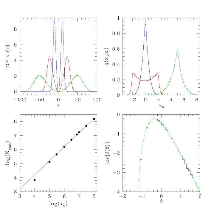
Figure 1: The panels in this figure show four different tests of our Monte Carlo code against known analytic solutions and Monte Carlo calculations by Loeb & Rybicki (1999). Upper left panel: The spectrum emerging from a uniform spherical gas cloud, in which Ly$\alpha$ photons are injected in the line center, $x=0$. The total line center optical depth, $\tau_{0}$ from the center to the edge is $10^{5}$ and $10^{7}$ for the narrowest (blue) and broadest (green) profile, respectively. The intermediate spectrum (red) corresponds to $\tau_{0}=10^{6}$. Overplotted as the black dotted line is the theoretically derived spectrum, eq. (9). The tests that are shown in the other panels are described in Appendix B. Upper right panel: The colored histograms are the redistribution functions, $q_{II}(x^{\prime},x)$, for $x=0$ (blue), $x=2$ (red) and $x=5$ (green), as extracted from the code. The solid lines are the analytic solutions given in Hummer (1962) and Lee (1974). Lower left panel: The total number of scatterings a Ly$\alpha$ photon undergoes before it escapes from a slab of optical thickness $2\tau_{0}$ as extracted from the code (circles). Overplotted as the red–solid line is the theoretical prediction by Harrington (1973). Lower right panel:. The spectrum emerging from an infinitely large object that undergoes Hubble expansion. The histogram is the output from our code, while the green–solid line is the (slightly modified) solution obtained by Loeb & Rybicki (1999) using their Monte Carlo algorithm.

$$R_{7}=\frac{3}{8}\int_{-1}^{\mu}(1+\mu^{\prime 2})d\mu^{\prime},$$ (7)

where $\mu\equiv{\vec{k}_{i}}\cdot{\vec{k}_{o}}$. Given ${\vec{k}_{i}}$, we have ${\vec{k}_{o}}=\mu{\vec{k}_{i}}+$ $(1-\mu^{2}){\vec{k}_{\perp}}$, where ${\vec{k}_{\perp}}$ is an arbitrary unit vector perpendicular to ${\vec{k}_{i}}$. ${\vec{k}_{o}}$ is calculated from ${\vec{k}_{o}}$ via a Lorentz transformation into the observer’s frame. Once ${\vec{v}_{a}}$ and ${\vec{k}_{o}}$ are known, $x_{o}$ can be calculated using eq. 3. After replacing $x_{i}$ and ${\vec{k}_{i}}$ by $x_{o}$ and ${\vec{k}_{o}}$, respectively, we return to step 3.

3.1.1 Accelerated Scheme

It is possible to speed up the code using a method described by Ahn et al. (2002). A critical frequency, $x_{\rm crit}$, defines a transition from ‘core’ to ‘wing’. Once a photon is in the core ($|x^{\prime}|<x_{crit}$), it is possible to force it (back) into the wing, by only allowing the photon to scatter off a rapidly moving atom. This is achieved by drawing $u_{\perp 1}$ and $u_{\perp 2}$ (Step 5. in § 3.1) from a truncated Gaussian distribution, which is Gaussian for $u>x_{\rm crit}$, but $0$ for $u<x_{\rm crit}$. To be more precise:

$$u_{\perp 1} =\sqrt{x_{\rm crit}^{2}-{\rm ln}[R_{11}]}\hskip 2.84526pt\cos(2\pi R_{10})$$

$$u_{\perp 2} =\sqrt{x_{\rm crit}^{2}-{\rm ln}[R_{11}]}\hskip 2.84526pt\sin(2\pi R_{10}),$$ (8)

where $u_{\perp 1,2}$ is again in units of $v_{\rm th}$.

The reason it is allowed to skip core scattering is that spatial diffusion occurs predominantly in the wings (see § 2). Skipping scattering events in the core effectively sets the mean free path of core photons to $0$. Clearly, $x_{\rm crit}=0$ restores the non–accelerated version of the code. Unless stated otherwise, in this paper we used $x_{\rm crit}=3$. We found that larger values of $x_{\rm crit}$ changed the appearance of the spectrum, especially the presence of the red peak (see below) was strongly affected.

3.2 The Tests

We performed various tests on the code, three of which are described in Appendix B. The other test is explicitly described here, since it involves a new analytic solution we derived in Appendix C. The test is similar to one generally done by other groups (e.g. Ahn et al., 2000, 2002; Cantalupo et al., 2005, ZM02), but differs in the geometry of the gas distribution. Ly$\alpha$ photons are injected at $x=0$ in the center of a uniform, non–absorbing, static sphere with the gas at $T=10$ ${}^{\circ}K\hskip 2.84526pt$, which corresponds to $a=1.5\times 10^{-2}$. The line center optical depth from the center to the edge of the sphere is $\tau_{0}$. In the upper left panel of Figure 1 the emergent spectra are shown for three different values of $\tau_{0}$: $\tau_{0}=10^{5},10^{6}$ and $10^{7}$ and compared to the analytic solution given below.

$$J(x)=\frac{\sqrt{\pi}}{\sqrt{24}a\tau_{0}}\Bigg{(}\frac{x^{2}}{1+{\rm cosh}\Big{[}\sqrt{\frac{2\pi^{3}}{27}}\frac{|x^{3}|}{a\tau_{0}}\Big{]}}\Bigg{)}$$ (9)

The derivation of this analytic solution for a sphere is completely analogous to the derivation given by Harrington (1973) and Neufeld (1990), and can be found in Appendix C. As mentioned in § 2, the emergent spectra are double–peaked and symmetric around the origin, with $x_{p}$ increasing with $\tau_{0}$. For a given value of $\tau_{0}$, $x_{p}=0.92(a\tau_{0})^{1/3}$ (vs. $x_{p}=1.06(a\tau_{0})^{1/3}$ for a slab). The spectra are normalized (as is the analytic solution) such that the area under all curves is $(2\pi)^{-1}$. The figure shows that the agreement is good. In Appendix B other tests are performed on the code that involve core scattering and a case in which the gas has bulk motions. Here, we briefly summarize these tests: In the upper right panel the redistribution functions, $q_{II}(x^{\prime},x)$, for $x=0$ (blue), $x=2$ (red) and $x=5$ (green), as extracted from the code are compared with the analytic solutions given in Hummer (1962) and Lee (1974) (solid lines). The total number of scatterings a Ly$\alpha$ photon undergoes before it escapes from a slab of optical thickness $2\tau_{0}$ as extracted from the code (circles) is shown in the lower left panel. Overplotted as the red–solid line is the theoretical prediction by Harrington (1973). In the lower right panel we show the spectrum emerging from an infinitely large object that undergoes Hubble expansion. The histogram is the output from our code, while the green–solid line is the (slightly modified) solution obtained by Loeb & Rybicki (1999, hereafter LR99) using their Monte Carlo code. As Figure 1 shows, the code passes all these tests well.

4 Deuterium

Although it has a low abundance, accounting for deuterium may be relevant when predicting spectra emerging from Ly$\alpha$ emitters. The resonance frequency of the deuterium Ly$\alpha$ absorption line is blueshifted by $82$ km s${}^{-1}\hskip 2.84526pt$with respect to that of hydrogen. For a gas at $T\equiv T_{4}\times 10^{4}$ K, this corresponds to $x_{D}\equiv+6.3\hskip 2.84526pt(T_{4})^{-1/2}$. According to eq. (2), the hydrogen optical depth at this frequency is reduced to $\tau_{x_{D},H}\sim 6.6\times 10^{-6}$ $\hskip 2.84526ptT_{4}^{1/2}\tau_{0}$. At this frequency, the photon is (by definition) exactly in the deuterium line center, and the optical depth due to deuterium is $\tau_{x_{D},D}=2^{1/2}[D/H]\tau_{0}$ $\sim 4.4\times 10^{-5}\tau_{0}$, where $[D/H]$ is the number of deuterium atoms per hydrogen atom, $[D/H]=3\times 10^{-5}$ (Burles & Tytler, 1998). The contribution of deuterium to the optical depth, $\tau_{x,D}/\tau_{0}$, is shown as a function of frequency in the range $x=3-10$ (red–solid line in Figure 2). The black–dotted line) shows the original $\tau_{x,H}/\tau_{0}$ given by eq. (2). The (blue–dashed line) shows the sum of the two. The gas is assumed to be at $10^{4}$ ${}^{\circ}K\hskip 2.84526pt$. Clearly there is a range in frequencies, $x\sim 5-8$, where deuterium dominates the optical depth and regulates the transfer of Ly$\alpha$ photons. Despite extensive research on Ly$\alpha$ radiative transfer, this detail has been neglected, to our knowledge, in all previous studies.

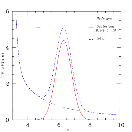
Figure 2: The contribution of a cosmological abundance of deuterium ($[D/H]=3\times 10^{-5}$) to the Ly$\alpha$ opacity for a gas at $T=10^{4}$ K. The ratio of the optical depth at frequency $x$ and frequency $x=0$, $\tau_{x,H}/\tau_{0}\equiv H(a,x)$, through static gas is shown. The black–dotted line is for hydrogen only ( and is given by eq. 2); the red–solid line is for deuterium only; the blue–dashed line is their sum. The figure shows that in the range $x=5-8$, deuterium dominates the opacity. For lower/higher temperatures, this spectral modification occurs at higher/lower values of $x$ with a relatively larger/smaller contribution from deuterium, respectively.

To include deuterium in our code we added the contribution of deuterium, $\tau_{x,D}$, to $\tau_{x}$. In addition to this, a step was added to the code following Step 4. (§ 3.1), that determines whether a scattering occurs by a hydrogen or deuterium atom. A random number $R_{D}$ was generated between 0 and 1. Let $P_{H}\equiv\tau_{x,H}/[\tau_{x,H}+\tau_{x,D}]$ be the probability that the Ly$\alpha$ photon is scattered by hydrogen. When $R_{D}\leq P_{H}$, the scattering is done by hydrogen, in which we proceed as described under Step 5. in § 3.1. Otherwise, the scattering is done by deuterium and its velocity vector is generated in exactly the same way, but with $a$ and $x$ replaced by $2^{1/2}a$ and $2^{1/2}[x-82\hskip 2.84526pt{\rm km}\hskip 2.84526pt{\rm s}^{-1}/v_{th}]$, respectively.

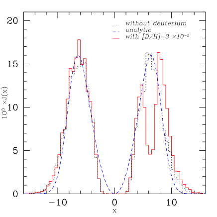
Figure 3: The effect of a cosmological abundance of deuterium ($[D/H]=3\times 10^{-5}$) on the spectrum emerging from a sphere with a center–to–edge column density of hydrogen of $N_{\rm HI}=1.2\times 10^{19}$ cm^-2. The reduced mean free path of Ly $\alpha$ photons in the deuterium line center inhibits their escape, which modifies the spectrum. For this plot, the gas temperature was assumed to be $10^{4}$ K.

Figure 3 demonstrates the impact of deuterium on the Ly$\alpha$ spectrum emerging from a uniform sphere in which the photons are injected at line center ($x=0$) in the sphere’s center. The gas is at $T=10^{4}$ ${}^{\circ}K\hskip 2.84526pt$and the total column of hydrogen from the center to the edge of the sphere is $N_{HI}=1.2\times 10^{19}$ cm^-2, yielding $\tau_{0}=7.3\times 10^{5}$ (eq. 1). The emerging spectrum is shown with (red–solid–histogram) and without (black–dotted–histogram) deuterium taken into account. The blue–dashed line is the theoretically predicted spectrum, eq (9). The reason the theoretical curve does not fit very well is that the product $a\tau_{0}=343$, while Neufeld (1990) requires $a\tau_{0}$ to be $a\tau_{0}\gtrsim 10^{3}$ for the theoretical curve to provide a good fit. The imprint deuterium leaves on the spectrum is strong. The main reason is that the presence of deuterium reduces the mean free path for photons near $x=x_{D}$, which reduces the probability that they escape the medium at this frequency. We find that even for a $10$ times lower deuterium abundance, the imprint in the spectrum is still noticeable.

For deuterium to leave an observable imprint in the spectrum, it should affect the frequencies at which a non-negligible fraction of Ly$\alpha$ photons emerges (as in Fig. 3). For $T_{4}=1$, for example, we expect deuterium to leave a spectral feature for columns in the range $N_{\rm HI}=10^{18}-10^{20}$ cm^-2, since this range would translate to $x_{p}\sim(a\tau_{0})^{1/3}\sim 3-12$. It is interesting that this corresponds to the range of column densities in Lyman limit systems. Because the columns studied in this paper are much larger, typically $10^{21}-10^{22}$ cm^-2, the spectral feature due to deuterium is much less prominent. Furthermore, bulk motions in the gas will most likely smear the absorption feature over a wide frequency range, which makes it even harder to observe in practise. A further challenge is that the frequency range of the deuterium feature corresponds to 3 thermal widths, or $v\sim 40$ km s^-1. To resolve this narrow feature, spectra are required with $R\sim 20000$. This resolution can be achieved with the High Resolution Echelle Spectrometer (HIRES) on Keck. Its detectability depends, however, on the total flux of Ly$\alpha$ emission. The brightest known Ly$\alpha$ blobs are $\sim 10^{-15}$ ergs s^-1 cm^-2 (Steidel et al., 2000), which is $\;\hbox to0.0pt{\lower 2.5pt\hbox{$\sim$}\hss}\raise 1.5pt\hbox{$<$}\;2$ orders of magnitude fainter than the sources successfully observed with this instrument. We plan to address the feasibility of detecting deuterium in more detail in future work.

5 Ly$\alpha$ Emission from Neutral Collapsing Gas Clouds without Stars or Quasars

5.1 Physics of Cloud Collapse and Ly$\alpha$ Generation

For gas to collapse inside its host dark matter halo, it must lose its gravitational binding energy. In the standard picture this binding energy is converted to kinetic energy, which is converted to thermal energy when the gas reaches the virial radius, where it is shocked to the virial temperature of the dark matter halo, $T_{\rm vir}$. When the cooling time is less than the dynamical time, the gas practically cools down to $10^{4}$ ${}^{\circ}K\hskip 2.84526pt$instantly. Since this gas is no longer pressure supported, it falls inward on a dynamical timescale (Rees & Ostriker, 1977). Haiman et al. (2000) argued that a large fraction of the cooling radiation is emitted in the Ly$\alpha$ line (see also the early work by Katz & Gunn 1991, who computed the Ly$\alpha$ cooling radiation in a hydrodynamical simulation). Birnboim & Dekel (2003) presented a refined version of the previous scenario, and used analytical arguments in combination with a 1-D hydro simulation to show that virial shocks do not exist in halos with $M\;\hbox to0.0pt{\lower 2.5pt\hbox{$\sim$}\hss}\raise 1.5pt\hbox{$<$}\;2\times 10^{11}M_{\odot}$ (which at $z=3$ translates to $v_{\rm circ}\;\hbox to0.0pt{\lower 2.5pt\hbox{$\sim$}\hss}\raise 1.5pt\hbox{$<$}\;130$ km s^-1). Consequently, the gas in these halos never gets shocked to the virial temperature and the gas is accreted ‘cold’ (also see Thoul & Weinberg, 1995).

The details of cloud collapse and the associated Ly$\alpha$ emission are unclear. In Birnboim & Dekel (2003)’s scenario, the gas falls unobstructed into the center, where its kinetic energy is converted to heat, which is radiated away in soft X-Rays. As a result, an HII region forms in which recombination converts $\sim 68\%$ of the ionizing radiation into Ly$\alpha$. The details of the gas distribution in the center and on the mean energy of the ionizing photons determine the radius of this HII region, and thus how centrally concentrated the Ly$\alpha$ emitting region is.

Haiman et al. (2000) describe an alternative scenario that is supported by 3-D simulations, that show that any halo is build up of mergers of pre-existing clumps. The denser colder clumps fall inwards, while experiencing weak secondary shocks from supersonic encounters with other density inhomogeneities. As a result, the clumps are continuously heated, which is balanced by cooling through Ly$\alpha$ emission. In the case the clumps fall in at a constant speed, all the gravitational binding energy of a clump is converted into heat which is radiated away in the Ly$\alpha$ line. The Ly$\alpha$ emissivity associated with this scenario is spatially extended.

The main difference in the above models is the degree of concentration of the Ly$\alpha$ emissivity. While we cannot realistically model the emissivity profiles ab-initio, we will below consider a wide range of profiles that should bracket the possibilities discussed above.

5.2 Modeling the Gas Kinematics and Ly$\alpha$ Emissivity Profile

Below, we define our model explicitly, and list the model parameters. We discuss the uncertainties of each parameter, and motivate the range of values we consider in each case. Input that is kept fixed in all models is the density distribution of the dark matter, $\rho_{D}(r)$, which is given by a NFW profile with concentration parameter $c=5$. The gas temperature is assumed to be $10^{4}$ K for all models. As discussed in § 8.2, changing the gas temperature does not affect our main results. The density distribution of the baryons, $\rho_{b}(r)$, is assumed to trace the dark matter at large radii, with a thermal core at $r<3R_{s}/4$ (see Maller & Bullock, 2004, their eq. 9-11, where $R_{s}=R_{\rm vir}/c$). Although the results are not presented in this paper, we found the effect of varying the concentration parameter $c$ to have no significant impact on our results.

The total (dark matter + baryons) mass range of the collapsing cloud, $M_{\rm tot}$, covered in this paper is $10^{10}-10^{13}M_{\odot}$. A related quantity is the circular velocity, $v_{circ}$. The upper limit on this mass range is set by simple cooling arguments: the cooling time of objects exceeding $10^{13}M_{\odot}$ exceeds the Hubble time (e.g Blumenthal et al., 1984). The lower limit corresponds to the mass that can collapse even in the presence of an ionizing background ($10^{10}M_{\odot}$ corresponds to $v_{\rm circ}\sim 50$ km s^-1 at $z=3$, see e.g. Thoul & Weinberg, 1996; Kitayama & Ikeuchi, 2000; Dijkstra et al., 2004). The redshift range at which the system virializes, $z_{\rm vir}$ covered in this paper is $z_{\rm vir}=3-6$. The lower limit is set by the redshift of the observed Ly$\alpha$ blobs which are candidates for cooling radiation. The upper limit is set by the opacity of the IGM which drastically increases beyond $z\gtrsim 6$ (e.g. Fan et al., 2002). Other input that is varied includes:

The velocity field, $v_{\rm bulk}(r)$, is given by a simple power law ${\rm v}_{\rm bulk}(r)=v_{\rm amp}[r/r_{vir}]^{\alpha}$. The velocity profile is uncertain; it can conceivably increase or decrease with radius. A spherical top-hat model would have $\alpha=1$ and $v_{\rm amp}=v_{\rm circ}$. In more realistic initial density profiles the mean density within radius $r$ decreases smoothly with radius, causing the inner shells to be decelerated more relative to the overall expansion of the universe. This enhances the infall speed at small $r$ relative to that in the top-hat model. The result of this is a flatter velocity profile, i.e $\alpha<1$. Accretion of massless shells onto a point mass results in $\alpha=-1/2$ (Bertschinger, 1985). Since it spans the range we can motivate physically, we study values of $\alpha$ in the range $\alpha\in[-0.5,1]$, but note $\alpha$ may in fact be $\;\hbox to0.0pt{\lower 2.5pt\hbox{$\sim$}\hss}\raise 1.5pt\hbox{$<$}\;0.5$. For cases with $\alpha<0$, the velocity diverges as $r\rightarrow 0$. This artificially boosts the emission at small $r$. To prevent this, these cases are modified to flatten at $r\lesssim r_{v}$:

$$v_{\rm bulk}(r)=v_{\rm amp}\Big{[}\frac{r_{v}+r}{r_{v}+r_{\rm vir}}\Big{]}^{\alpha}.$$ (10)

When $r\gg r_{v}$, $v_{\rm bulk}=v_{\rm amp}[r/r_{\rm vir}]^{\alpha}$ and when $r\rightarrow 0$, then $v_{\rm bulk}\rightarrow v_{\rm max}$. We set $v_{\rm max}=2v_{\rm amp}$, which uniquely determines $r_{v}$. The amplitude of the velocity field $v_{\rm amp}$ is also varied between $0$ and $2$ $v_{\rm circ}$.

The emissivity, $j(r)$, which we take to be either ‘extended’ or ‘central. The extended case refers to the scenario sketched by Haiman et al. (2000), in which the gas continuously emits a fraction $f_{\alpha}$ of the change of its gravitational binding energy in the Ly$\alpha$ line. The emissivity as a function of radius $j(r)$, in ergs s^-1 cm^-3, is then given by

$$j(r)=f_{\alpha}\frac{G\hskip 2.84526ptM_{\rm tot}(<r)\hskip 2.84526pt\rho_{b}}{r^{2}}\frac{dr}{dt},$$ (11)

where $M_{\rm tot}(<r)$ is the total mass enclosed within radius $r$, $\rho_{b}$ the mass density of baryons at radius $r$ and $dr/dt$ is simply $v_{bulk}$, the speed at which the gas at radius $r$ is falling in. We assume $f_{\alpha}$=1, which reflects extreme cases in which all gravitational binding energy is converted into Ly$\alpha$. The results given below scale linearly with $f_{\alpha}$.
The ‘central’, $j(r)=\mathcal{K}\delta(r)$, models represent the extreme version of the scenario sketched by Birnboim & Dekel (2003), in which all Ly$\alpha\hskip 2.84526pt$is only generated in the center. Alternatively, these central models may represent any model in which a central Ly$\alpha\hskip 2.84526pt$emitting source is surrounded by a neutral collapsing gas cloud. We determine $\mathcal{K}$ from we the total Ly$\alpha$ luminosity, given by $L_{{\rm ly}\alpha}\equiv\int\hskip 2.84526ptdVj(r)$. For simplicity, we set $L_{{\rm ly}\alpha}$ equal in the extended and central models with otherwise identical parameters.

A brief summary of all models studied in this paper is given in Table 2 in Appendix A. All results below are obtained by setting $r_{\rm max}=r_{\rm vir}$ (§ 3.1), which implies that we ignore the Ly$\alpha$ transfer beyond the virial radius. The impact of the IGM surrounding the virialized halo can vary from location to location (e.g. due to stochastic density and ionizing background fluctuations and also from the proximity effect near bright QSOs). We take the approach of studying the effects of scattering in the virialized halo and in the IGM separately. In this paper, we only compute the Ly$\alpha$ spectra as they emerge at the surface of the halos at $r_{\rm vir}$ with a brief discussion of the effect of the IGM in § 8.1. the IGM is discussed in more detail in PaperII.

6 Results

Before discussing the spectral features and surface brightness profiles, it is useful to express the total Ly$\alpha$ luminosity, $L_{{\rm Ly}\alpha}$ ($L_{{\rm ly}\alpha}\equiv\int\hskip 2.84526ptdVj(r)$, § 5.2), as a function of our model parameters:

$$\frac{L_{{\rm Ly}\alpha}}{10^{42}}=0.66\hskip 2.84526pt\Big{(}\frac{M_{\rm tot}}{10^{11}}\Big{)}^{\frac{5}{3}}\Big{(}\frac{v_{amp}}{v_{\rm circ}}\Big{)}\Big{(}\frac{1+z_{\rm vir}}{5}\Big{)}^{\frac{5}{2}}\Big{(}\frac{2-\alpha}{1.75}\Big{)}^{1.2}\hskip 2.84526pt\frac{{\rm ergs}}{{\rm sec}}.$$ (12)

The scalings of $L_{{\rm ly}\alpha}$ with $M_{\rm tot}$ and $v_{amp}$ and $(1+z_{\rm vir})$ are exact. The $\alpha$ dependence is a fit, that is accurate to within $10\%$, over the range $\alpha\in[-0.5,1]$. Note that equation (12) can be written as:

$$\frac{L_{{\rm Ly}\alpha}}{10^{42}}=0.66\hskip 2.84526pt\Big{(}\frac{{\rm v}_{\rm circ}}{116\hskip 2.84526pt{\rm km}\hskip 2.84526pt{\rm s}^{-1}}\Big{)}^{5}\Big{(}\frac{v_{amp}}{v_{\rm circ}}\Big{)}\Big{(}\frac{2-\alpha}{1.75}\Big{)}^{1.2}\hskip 2.84526pt\frac{{\rm ergs}}{{\rm sec}}.$$ (13)

The dependence of $L_{{\rm Ly}\alpha}$ on $v_{\rm circ}$ can be understood from the following scaling relations: $L_{{\rm Ly}\alpha}\propto U/t$ ($U$ is the total gravitational binding energy and $t$ is the timescale over which it is released, which is taken to be the dynamical timescale of the halo) $\propto U/(R_{\rm vir}/v_{\rm circ})$ $=v_{\rm circ}U/R_{\rm vir}$ $\propto v_{circ}M^{2}/R_{\rm vir}^{2}$ $\propto v^{5}_{\rm circ}$, where we used that $U\propto GM^{2}/R_{\rm vir}$ and $v^{2}_{\rm circ}=GM/R_{\rm vir}$.

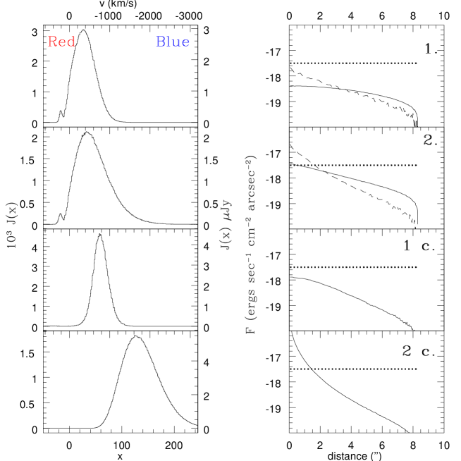
Figure 4: Properties of the Ly$\alpha$ emission emerging from our four fiducial models (models 1., 2, 1 c and 2 c) of neutral collapsing gas clouds. The left panels show spectra in which the lower horizontal axis shows the normalized frequency variable $x$. The upper horizontal axis shows what velocity offset this frequency corresponds to. Values of $x>0$ correspond to higher frequencies, or lower redshifts, which corresponds to lower recessional velocities. The left vertical axis shows the normalized flux, while the right vertical axis has the flux density in $\mu$Jy. Processing by the IGM is ignored in the plot. The right panels show the corresponding surface brightness distribution. The thick dotted horizontal line corresponds to the detection limit in a recent survey for Ly$\alpha$ blobs by Matsuda et al. (2004). The model number is shown in the top right corner. The details of each model can be found in Table 2. The black–dashed line, in the upper two panels in the right column, is the surface brightness profile that would emerge, in the absence of scattering. For the central models, this line corresponds to a $\delta-$function at $0$”, and is therefore not shown. For all infall models, the Ly$\alpha$ line emerges with a net blueshift.

In § 6.1 we show some examples of Ly$\alpha$ spectra and surface brightness profiles emerging from several models. The main purpose of this is to gain basic insight into the Ly$\alpha$ radiation emerging from neutral, collapsing gas clouds with no star formation or quasar activity. In § 6.2 the dependence of these properties on the model parameters is studied in more detail. Our main findings are summarized and and qualitatively explained in § 6.3.

6.1 Examples of Intrinsic Spectra and Surface Brightness Profiles

We show the emerging spectrum (left panels) and surface brightness profile (right panels) for models 1., 1 c, 2 and 2 c. in Figure 4. These models cover the full range of velocity profiles and Ly$\alpha$ emissivities. The model number associated with a given row shown in the top right corner of the right panels. The lower horizontal axis on the left column denotes the usual frequency variable $x$, which is converted to a velocity offset (in the Ly$\alpha$ emitter’s rest–frame) from the line center, on the upper axis. Note that positive values of $x$ correspond to higher energies, or bluer photons. The vertical axis on the left side has units which are such that the area under the curves corresponds to $(2\pi)^{-1}$ ( as in Fig. 1). The vertical axis on the right indicates the physical flux density in units of $\mu$ Jy (ignoring scattering in the IGM, see § 8.1). The right panels panels show the surface brightness profiles. The horizontal axis denotes the impact parameter, measured in ^′′. The units of the surface brightness on the vertical axis are ergs s^-1 cm^-2 arcsec^-2. The thick dotted horizontal line is the detection limit in the recent survey by Matsuda et al. (2004).

First, we focus on the spectra which show that the Ly$\alpha\hskip 2.84526pt$radiation escapes the collapsing protogalaxy predominantly blue shifted for all models. The extended models are not as blue as the central models, and they contain a faint red peak. We quantify the prominence of the red peak through the ratio $[B]/[R]$, defined as the number of photons in the blue peak over the number of photons in the red peak.

Second, we focus on the surface brightness distribution. Model 1. has a very flat profile, $F(\theta)\propto\theta^{-a}$, with $a\sim 0.5$. Model 2. has a steeper profile with $a\sim 1.0$ and the central surface brightness is increased above Matsuda et al. (2004)’s detection limit. The profile that would emerge in the absence of scattering is overplotted as the dashed curves. These curves illustrate the extent to which the surface brightness distribution becomes shallower because of scattering. The profiles for models 1 c. and 2 c. are more centrally concentrated ($a\sim 2$), which can be viewed simply as an extension of the trend seen in the profiles of models 1. and 2.: A steeper emissivity profile translates to a steeper surface brightness profile.

6.2 Impact of Model Parameters on the Emitted Ly$\alpha$ Features

Here we discuss the impact of varying the model parameters described in § 5.2 on on the following properties of the emergent spectrum: (i) net blueshift of the blue peak, (ii) FWHM of the blue peak, (iii) the location of the red peak (if any), (iv) the ratio $[B]/[R]$, and (v) the surface brightness profiles.

6.2.1 Spectral Shape: Peak Morphology-The Blue Peak

Figure 5: This figure shows the morphology of the blue peak as a function of various model parameters. The location of the maximum of the blue peak (triangles) and its FWHM (circles) as a function of 3 parameters for the extended (upper panel) and central (lower panels) models. The left panel, middle panel and right panel shows the dependence on $\alpha$, $v_{\rm amp}$ and the optical depth $\tau$. The optical depth $\tau$ is normalized to $\tau_{1}$, which is the optical depth from center to edge of model 1. (see text). These trends suggest degeneracies will exist between the quantities $\tau$, $\alpha$ and $v_{\rm amp}$ - for example, larger infall velocities can be mimicked by larger column densities and vice versa (and result in a larger blueshift of the Ly$\alpha$ line).

In Figure 5. we show the frequency offset of the blue peak’s maximum (triangles) and its FWHM (circles) as a function of three parameters: $\alpha$ (left panels), $v_{\rm amp}$ ( middle panels) and the optical depth $\tau$ from the center to the edge of the object (right panels). The upper and lower row of panels represents extended and central models, respectively.

The left panels show that for the extended models, the dependence of the location of the maximum on $\alpha$ is weak, while its FWHM is slightly more affected by $\alpha$ (which is not surprising, as we notice that the blue tail is more pronounced in the spectrum of model 2. than in model 1. in Fig. 4). On the other hand, the dependence on $\alpha$ is very strong for the central cases (which is also evident from the lower two rows in Figure 4).
The central panels show that for the extended models the FWHM depends more strongly on $v_{\rm amp}$ than the peak’s location. For the central models, the dependence of both quantities on $v_{\rm amp}$ is weaker than their dependence on $\alpha$. Also, the dependence of the FWHM on $v_{\rm amp}$ for the central models is slightly weaker relative to that of their extended counterparts.
The right panels of Figure 5 shows the location of the maximum of the blue peak and its FWHM for three different optical depths, $\tau$. The optical depth is normalized to that of model 1., denoted by $\tau_{1}$. All models are identical in their dark matter and gas properties, but the Ly$\alpha$ absorption cross section is decreased and increased by a factor of $10$ for the point with $\tau/\tau_{1}$ $=0.1$ and $10.0$, respectively. The figure demonstrates clearly that the blue peak’s morphology is strongly affected by the value of $\tau$. Both the FWHM and velocity shift of the Ly$\alpha$ line increase with $\tau$. These trends suggest that degeneracies will exist between the values of $\tau$, $v_{\rm amp}$ and $\alpha$ - for example, larger infall velocities can be mimicked by larger column densities and vice versa.

6.2.2 Spectral Shape: Peak Morphology-The Red Peak

Figure 6: The location of the maximum of the red peak (-circles) and the minimum in the spectrum (-triangles) as a function of $v_{\rm amp}$. The dotted line corresponds to the curve $v=v_{\rm amp}$. Despite the fact that the included models vary in mass, redshift and $\alpha$, the correlation is obvious, which suggests it is a generic property of the extended models. The location of the red peak potentially measures the gas infall speed.

Figure 6 shows the location of the dip (circles) and the maximum of the red peak (triangles) as a function of the amplitude of the velocity field for various models that vary in mass, redshift and their assumed velocity field. The dotted line denotes $v=v_{\rm amp}$. The exact parameters used for these models used in the plot can be read off from Table 2.

The relation between $v_{\rm amp}$ and the location of the peak and dip is evident. Beyond $v_{\rm amp}\sim 360$ km s^-1 the correlation breaks down. The reason is that the red and the blue peak merge for large $v_{\rm amp}$ (see Fig 5 and Fig 7 and their discussion below). The correlation holds for a wide range of models, which we take as evidence for it being a generic property of the extended models.

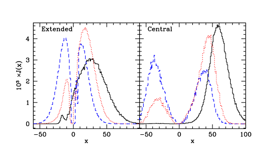
Figure 7: The effect of bulk motions in the gas on the emerging Ly$\alpha$ spectrum is shown for the extended (left panel) and central (right panel) cases. The panels contain normalized spectra for three models that only differ in the amplitude of the velocity field. The black–solid line in the left/right panel corresponds to model 1./1 c., respectively. The red dotted lines and blue dashed line correspond to the same models with $v_{\rm amp}$ reduced to $0.25v_{\rm circ}$ and 15 c.) and $v_{\rm amp}=0$, respectively. The red peak becomes smaller with increasing infall speed.

Figure 8: The ratio of the number of photons in the blue and red peak, $[B]/[R]$, as a function of various parameters. The fiducial model is model 1. (see Table 2). Variation with: upper left panel: mass, upper right panel: redshift (In this panel only, we include the scattering in the IGM, since it introduces a strong redshift dependence, see § 8.1), lower right panel: $v_{\rm amp}$, lower left panel: $\alpha$. The red peak’s prominence is enhanced towards higher redshifts, lower masses and lower infall velocities.

As mentioned in § 6.1 the blue to red ratio, $[B]/[R]$ quantifies the prominence of the red peak. First we demonstrate how the transition occurs from a double peaked symmetric spectrum, known from the static cases, to the asymmetric spectra, that are associated with bulk motions. The left and right panel of Figure 7 contains the (normalized) spectrum of models 1. and 1 c., respectively, as the black–solid lines. The red–dotted lines correspond to the same models, in which the amplitude of the infall velocity has been reduced to $0.25v_{\rm circ}$. The blue dashed lines correspond to $v_{\rm amp}=0$ (actually, $v_{\rm amp}=10^{-6}v_{\rm circ}$, because for $v_{\rm amp}=0$ there is no emission for the extended cases according to eq. 11).

The slight asymmetry that is present in both static cases, is intriguingly enough, due to deuterium. Deuterium also leaves a sharp feature at $x=x_{D}$ in the static, extended, case. The effect of deuterium on the other spectra was found to be negligible. Figure 7 shows that $[B]/[R]$ increases strongly with $v_{\rm amp}$ for both the central and extended models. In the central cases, the blue and red peak remain well defined and separated as the amplitude of the infall velocity is increased. However, the amplitude of the red peak falls quickly to be undetectable. For the extended cases, the FWHM of the blue peak increases, and that of the red peak decreases, until the peaks merge. The minimum in the spectrum that separates the blue and the red peak moves to redder frequencies with increasing $v_{\rm amp}$.

Figure 8 shows the value of $[B]/[R]$ as a function of $z_{\rm vir}$ (upper-right panel), $v_{\rm amp}$ (lower-right panel), $\alpha$ (lower-left panel) and $M_{\rm tot}$ (upper-left panel). The circles refer to the extended models, whereas the open stars refer to the central models.
The upper-left panel shows that $[B]/[R]$ increases strongly with mass. The upper-right panel shows that $[B]/[R]$ decreases strongly with $z_{\rm vir}$. In this panel only, we included the impact of the IGM, because the IGM introduces a strong z-dependence. A discussion of how the IGM was incorporated is delayed to § 8.1. The lower-right panel shows that the value of $[B]/[R]$ increases with the amplitude of the velocity field $v_{\rm amp}$. For sufficiently large $v_{\rm amp}$, the red peak is absorbed in the blue peak (see Fig 5), in which case $[B]/[R]\rightarrow\infty$. The lower-left panel shows that for the extended models $[B]/[R]$ is relatively insensitive to the value of $\alpha$. For the central models, no photons emerged on the red side of the line for $\alpha\leq 0.25$, causing $[B]/[R]\rightarrow\infty$.
These results suggest that the secondary red peak may be detectable in the spectra of (proto) galaxies, provided the Ly$\alpha$ emissivity is spatially extended. Furthermore, the red peak may be more easily detectable towards higher redshift. If detected, the location of the red peak gives a potentially useful measure of the gas infall speeds.

6.2.3 The Surface Brightness Profile

Figure 9: The surface brightness as a function of angular distance in ^′′ from the center of the Ly$\alpha$ image. The upper and lower panels represent extended and central models, respectively. Each panel corresponds to a different mass, which is given in units of $10^{11}M_{\odot}$ in the upper right corner of each panel. The velocity profiles have slopes $\alpha=$ $-0.5$ (steepest curve), $0.25$ and $1.0$ (shallowest curve). The figure shows that the surface brightness profile becomes flatter with increasing mass. For a given mass, the exact slope is determined by how centrally concentrated the Ly$\alpha$ emissivity is.

Finally, we focus on the impact of varying the input parameters on the emerging surface brightness profile. Figure 9 shows the surface brightness distribution as a function of $M_{\rm tot}$, $\alpha$ and $j(r)$. The upper and lower panels are associated with extended and central models, respectively. Each panel contains three models for one particular mass, $M_{\rm tot}$, which is given in the top right corner in units of $10^{11}M_{\odot}$. In all panels, the lowermost and uppermost curve corresponds to $\alpha=1.0$ and $-0.5$, respectively (also see Fig. 4), the middle curve has $\alpha=0.25$. Figure 9 shows that the surface brightness profile flattens with increasing mass and $\alpha$.

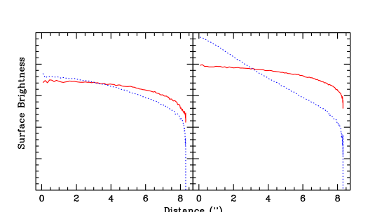
Figure 10: This figure shows the frequency dependence of the surface brightness profile for the extended models. The surface brightness profile for the bluest (dotted blue line) and reddest (red solid line) 15$\%$ of the photons are shown. The left and right panel corresponds to models 1. and 2., respectively. The figure shows that for collapsing gas clouds, the bluest Ly$\alpha$ photons may emerge more centrally concentrated than the reddest Ly$\alpha$ photons.

Figure 10 shows the surface brightness profiles associated with model 1. (left panel) and model 2. (right panel). The two profiles are constructed from the reddest $15\%$ (red solid line) and the bluest $15\%$ (blue dotted line) of all Ly$\alpha$ photons. The bluest 15$\%$ is more concentrated, especially for model 2., which has $\alpha=-0.5$. This suggests that steepening of the surface brightness profile towards bluer wavelengths within the Ly$\alpha$ line may be useful to diagnose gas infall. The amount of steepening may constrain the infall velocity profile.

6.3 Summary of Intrinsic Ly$\alpha$ Properties

The results obtained above can best be summarized as:

• Result 1. For all models, the Ly$\alpha$ radiation emerges predominantly blueshifted, typically by $500-3000$ km s^-1.This can be explained as follows: 1) Photons propagating outwards in a collapsing gas cloud experience a net blueshift, because of energy transfer from the infalling gas to the photons 2) Blueshifted Ly$\alpha$ photons that are propagating outwards appear even bluer (and thus further in the wing) for the infalling gas, which facilitates their escape, while the reverse is true for redshifted photons. These two effects yield a suppressed red and enhanced blue peak.

• Result 2. The spectra of the central models are systematically bluer than those of the extended models. This result reflects that Ly$\alpha$ photons that are inserted deeper inside the collapsing gas cloud, obtain a larger average blue shift as they propagate outwards. That is, they have to traverse a larger column of neutral infalling gas, which allows more energy to be transferred from gas to photons, which results in a larger average blue shift.

• Result 3. The ’extended’ models typically have an additional faint red peak in the spectrum separated by a minimum in the spectrum (the ’dip’). Both the location of the maximum of the red peak and the dip are uniquely determined by the infall velocity of the outermost gas layers. The reason for this is that some of the red Ly$\alpha$ photons that are propagating outwards are exactly at resonance in the frame of the infalling gas, which significantly reduces their escape probability and produces the observed dip. The dip in the spectrum is therefore strongly linked to the gas’ infall velocity (at the outermost gas shells). In § 8.2 we point out that despite the simplified nature of our models, in which the only bulk motions in the gas are radial and always in-flowing, this result is unlikely to change for more realistic, more complex gas distributions.

• Result 4. The Ly$\alpha$ properties of the ’central’ models depend more sensitively on $\alpha$ than those of the ’extended’ models, with the average blueshift of the spectrum strongly increasing with decreasing $\alpha$. This reflects that all Ly$\alpha$ photons in the central models are exposed to scattering by the gas in the central regions. Changing $\alpha$ from $1.0$ to $-0.5$, enhances $v_{\rm bulk}$ by a factor of $(r_{\rm vir}/r)^{1.5}$, which obviously becomes very large at small radii ($r\ll r_{\rm vir}$). Due to the enhanced infall velocity at small radii, more energy can be transferred from the gas to the photons in models with low values of $\alpha$, which results in a larger average blue shift of the Ly$\alpha$ line.

• Result 5. The prominence of the red peak, quantified by the ratio $[B]/[R]$, increases with decreasing infall velocity, mass and total Ly$\alpha$ optical depth. The ratio $[B]/[R]$ decreases with redshift for fixed other model parameters. These trends are easily understood: The larger the infall velocity, and the total Ly$\alpha$ optical depth, the more energy is transferred from gas to photons as the photons work their way outwards. This results in a more prominent blue peak and larger $[B]/[R]$. As explained above, increasing $\alpha$ reduces the number of very blue photons and, subsequently, $[B]/[R]$. The increase of $[B]/[R]$ with mass is caused by the increase of both the infall velocity, and the total Ly$\alpha$ optical depth with mass. The decrease of $[B]/[R]$ with redshift caused by the increased probability with redshift for photons on the blue side of the line center to be scattered out of our line of sight in the IGM. This is discussed in more detail in § 8.1.

• Result 6. The surface brightness profiles for the extended models are typically flat, $\partial F/\partial{\rm ln}\theta=-1$ to $-0.5$, with an increasing flatness with increasing mass and $\alpha$. The same trends are seen for the central models, which consistently have steeper surface brightness distributions with $\partial F/\partial{\rm ln}\;\hbox to0.0pt{\lower 2.5pt\hbox{$\sim$}\hss}\raise 1.5pt\hbox{$<$}\;-2$. One reason that the surface brightness profiles of the extended models become flatter with increasing $\alpha$ is that the intrinsic emissivity becomes flatter with increasing $\alpha$ (see Fig 4). This is not the only reason though, since the same trend is seen among the central models, which have identical $j(r)$ (apart from the amplitude). As was mentioned above, for lower values of $\alpha$ the number of very blue Ly$\alpha$ photons is enhanced, which increases the steepness of the surface brightness profile (see result 7. and its explanation below). The flattening of the surface brightness profile with mass is caused by: 1) The projected emissivity on the sky becomes increasingly shallow with mass, which is due to the mass dependence of the virial radius (for the extended models). 2) The Ly$\alpha$ optical depth increases with mass, which reduces the probability that photons propagate through the outer gas layers without being scattered.

• Result 7. A flattening of the surface brightness profile towards longer wavelengths within the Ly$\alpha$ line is indicative of infall. This can be explained as follows: the bluest photons emerge mainly from the center (as argued above) and are unlikely to get scattered in the outer gas layers. This is because these photons appear even bluer in the frame of the infalling gas, and thus further in the line wing. The reverse is true for the reddest photons, which appear much closer to the line center in the frame of the infalling gas and therefore likely scattered in the outermost gas layers. This produces a more diffuse appearance of the reddest photons compared to that of the bluest.

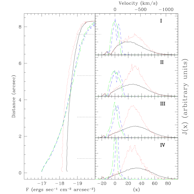
Figure 11: This figure displays the Ly$\alpha\hskip 2.84526pt$surface brightness distribution (left panel) and spectra emerging (right panels) from a collapsing gas cloud containing an ionizing source for four different ionizing luminosities. The spectra in the different panels are centered on the impact parameter indicated by the black–dotted lines. Model 1. is represented by the black–solid line ($L_{\rm ion}=0$). The red–dotted line, blue–dashed line and green–long–dashed line corresponds to model 1. plus an additional central ionizing source with $L_{\rm ion}=5\times 10^{42}$ ergs s^-1, $L_{\rm ion}=10^{43}$ and $10^{46}$ ergs s^-1, respectively. As $L_{\rm ion}$ increases, the spectral line becomes narrower and more symmetric around the line center.

7 Fluorescent Ly$\alpha$ Emission from Self-Ionized Protogalaxies

In this section, we focus on the observable properties of fluorescent Ly$\alpha$, such as its surface brightness distribution and its spectrum. For this purpose, an ionizing point source was inserted at the center of our sphere. Its total flux in ionizing photons is $L_{\rm ion}$ (in ergs s^-1) and its spectrum is a power law of the form $J(\nu,r)=J_{0}(r)(\nu/\nu_{L})^{\beta}$. The slope $\beta$ depends on the nature of the ionizing sources. We choose $\beta=1.7$, for the point source to represent a quasar. The value of $J_{0}(r)$ is obtained by $J_{0}(r)=(\beta-1)L_{\rm ion}/[16\nu_{L}\pi^{2}r^{2}]$. The standard equations of photoionization equilibrium were solved numerically with the code. The optical depth to the first shell was assumed to be $0$. This was used to calculate its neutral fraction of hydrogen. This allows the optical depth to the next shell to be computed, which also determines its neutral fraction. This procedure is repeated until the outer shell is reached. The resulting changes in the intrinsic Ly$\alpha$ spectrum are presented below.

7.1 Impact of a Central Ionizing Source on the Properties of the Emerging Ly$\alpha$ Emission

In the presence of an ionizing source we set the Ly$\alpha$ emissivity to be given by:

$$j(r)=\mathcal{F}_{\alpha}\alpha_{B}[1-x_{H}(r)]^{2}n_{H}^{2}(r)\hskip 2.84526pth\nu_{0}+f_{\alpha}\frac{G\hskip 2.84526ptM_{\rm tot}(<r)\hskip 2.84526pt\rho_{b}}{r^{2}}\frac{dr}{dt}$$ (14)

where $\mathcal{F}_{\alpha}$ is the average number of Ly$\alpha$ photons produced per recombination, which is $\sim 68\%$ for case B and $\sim 42\%$ for case A recombinations. Case A/B applies when the gas is optically thin/thick to all Lyman series photons, respectively. The second term is the same as used for the extended cooling models (eq. 11). The main reason for keeping this term is to make the transition from the previous extended models to the current models smooth.

The gas in model 1. becomes fully ionized at $L_{\rm ion}=10^{43}$ ergs s^-1. We caution that this estimate ignores small–scale gas clumping. If we denote the clumping factor by $C\equiv\langle\rho^{2}\rangle/\langle\rho\rangle^{2}$, then this transition to full ionization occurs at $\sim C$ times higher ionizing luminosity (which would allow for $\sim C$ times higher Ly$\alpha$ luminosity) .

Increasing $L_{\rm ion}$ beyond this value, merely reduces the residual neutral fraction, and consequently, $N_{\rm HI}$. The ‘phase transition’ from neutral to fully ionized dramatically affects the emerging Ly$\alpha$ spectrum. In Figure 11 we show the Ly$\alpha$ spectrum and surface brightness distribution for four values of $L_{\rm ion}$: $L_{\rm ion}=0$ (black–solid line), $L_{\rm ion}=5\times 10^{42}$ ergs s^-1 (red–dotted line), $L_{\rm ion}=10^{43}$ ergs s^-1 (blue–dashed line) and $L_{\rm ion}=10^{46}$ ergs s^-1 (green–long–dashed line). The results are presented differently than above: The left panel shows the surface brightness distribution rotated by 90^∘. The right panels show spectra of these models at four different impact parameters, $\theta$, indicated by the horizontal dotted lines. For example, the lowest panel shows the spectrum emerging from $\theta\sim 0-2^{\prime\prime}$, the second lowest panel shows the spectrum emerging from $\theta\sim 2-4^{\prime\prime}$, etc. The main reason for presenting the data in this fashion is to study the variations in the spectra across the object. Note that the spectra are arbitrarily scaled for visualization purposes.

We note that in the the absence of an ionizing source, the spectrum (black–solid line) is fairly constant across the object, the central region being slightly bluer. For low ionizing luminosities, $L_{\rm ion}=5\times 10^{42}$ ergs s^-1, photo-ionization enhances the Ly$\alpha$ emission from the central regions. Enhanced emission in the center enhances the number of photons in the bluest parts of the spectrum (§ 6.3), and steepens the surface brightness profile (observation 6. in § 6.3). These are indeed the trends that can be seen in Figure 11. When $L_{\rm ion}$ is increased by a further factor of two, the gas sphere as a whole is fully ionized, which produces several effects. The overall blueshift of the spectrum (blue–dashed line ) almost completely vanishes, and its FWHM is significantly smaller. The main reason is the reduced column of neutral hydrogen, which reduces the importance of broadening of the Ly$\alpha$ line by resonant scattering. Instead, the broadening is determined by the bulk velocity of the gas, despite the fact that each Ly$\alpha$ photon scatters $\sim 10^{4}$ times before it escapes. The reason that the Ly$\alpha$ spectrum is barely affected by scattering, is that each Ly$\alpha$ photon mainly scatters near the site of its creation, where the photon is at resonance. A chance encounter with a rapidly moving atom can put the photon in the wing of the line, which allows it to escape in a single flight from the local resonant region (in which the optical depth is $\tau_{0}\sim 10^{3}$-well within the regime of moderate opacities, Adams, 1972). These photons escape this region in a typical symmetric double peaked profile around the local line center. Velocity gradients in the gas facilitate the photon’s escape from the rest of the object, effectively without ’seeing’ shells at other radii. The frequency with which the photon finally emerges at the virial radius therefore does contain information on the bulk velocity of the site where the photon was generated. The double peak in the emission line in regions I-III is a consequence of this local resonant scattering. The main reason for the enhanced prominence of the dip at large impact parameters is that the velocity gradient projected along the line of sight is smaller there, which increases the total column of hydrogen a Ly$\alpha$ photon effectively sees.

The reason that the spectrum from region IV is narrower is that this spectrum mainly contains photons that emerge from the central regions, in which the bulk infall velocity is low ($\alpha=1.0$). The effect of the velocity field and $L_{\rm ion}$ ion the emerging spectrum is investigated in more detail in § 7.2.

7.2 Constraints from Ly$\alpha$ Emission on Gas Kinematics in the Presence of a QSO

In the previous section we argued that the gas kinematics can be constrained by the Ly$\alpha$ emission despite the possibility that the Ly$\alpha$ photon scatters up to $\sim 10^{4}$ times. In this section we show that, although the amplitude of the bulk velocities in the gas can be constrained well by the gas, the sign is much harder to determine, since the emerging spectra for infall and outflow are almost identical for fully ionized gas. In this section, we ignore contribution from cooling to the emissivity; the second term on the RHS in equation (14) is set to 0. The reason is that we want to explore the similarities of the effects of scattering, so we prefer to adopt the same emissivity profiles.

In Figure 12 we show spectra at four different impact parameters for three different models. The blue–dashed lines represent model 1. containing a central ionizing source with $L_{\rm ion}=10^{43}$ ergs s^-1 (as in Fig. 11). These spectra are compared to the no–scattering profiles, which refer to the profiles that would be observed if the gas were transparent to Ly$\alpha$ (shown as black–solid lines). The red–dotted lines represent a model in which the sign of $v_{\rm amp}$ is reversed. Each panel contains the spectra at the impact parameter indicated by the roman numerals in the top–right corner (as in Fig. 11).

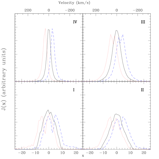
Figure 12: This figure shows the Ly$\alpha$ spectra emerging from optically thin outflowing and infalling gas. Each panel corresponds to the impact parameter indicated by the roman letter (as in Fig. 11). The spectra shown by the blue-dashed lines represent a photo-ionized infall model, while red–dotted lines represent the outflow models in which the sign of $v_{\rm amp}$ is reversed. The black–solid lines represent both infall and outflow models in the absence of scattering. The figure shows that when the gas is optically thin to Ly$\alpha$ photons, $\tau_{0}\;\hbox to0.0pt{\lower 2.5pt\hbox{$\sim$}\hss}\raise 1.5pt\hbox{$<$}\;10^{3}$, infall and outflow models can produce nearly identical Ly$\alpha$ spectra, except for a small shift in frequency.

The only prominent difference between all spectra, is that the models in which scattering occurs are shifted by several Doppler widths relative to the no-scattering spectrum. Infall and outflow models are slightly blue and redshifted shifted, respectively. The reasons for this shift have been discussed in § 6.3.

Although not shown in this paper, we found the surface brightness distributions for the optically thin infall and outflow models to be the identical (also see ZM02, who found the same). This leads to the conclusion that for gas that is only moderately thick to Ly$\alpha$ scattering, $\tau_{0}\;\hbox to0.0pt{\lower 2.5pt\hbox{$\sim$}\hss}\raise 1.5pt\hbox{$<$}\;10^{3}$, the Ly$\alpha$ spectrum can be used to determine its velocity dispersion, despite the fact that Ly$\alpha$ photon up may scatter up to $10^{3}-10^{4}$ times. However, the sign of the velocity field can only be determined when the exact Ly$\alpha$ line center is known, to an accuracy of $\sim 10$ km s^-1 (which is probably not possible in practice). This introduces an ambiguity in the interpretation of the Ly$\alpha$ blob found around a $z=3$ quasar by Weidinger et al. (2004, 2005). Although they attribute the observed spectra and surface brightness profiles to gas infall, our results suggest that outflowing gas can produce similar characteristics. We will explore this issue in more depth in paper II.

8 Discussion

8.1 The IGM Transmission

As mentioned in § 5.2, we have focussed on the intrinsic Ly$\alpha$ emission from collapsing protogalactic gas clouds. The subsequent Ly$\alpha$ transfer through the IGM, which is defined to lie beyond the virial radius, has been ignored so far. Even though the IGM is almost fully ionized at most redshifts considered in this paper, a small residual neutral fraction is enough to scatter some fraction of the Ly$\alpha$ photons from our line of sight. For an IGM that is comoving with the Hubble flow, the mean transmission is 1 and $\langle e^{-\tau}\rangle$ redward and blueward of the line center, respectively (e.g. Madau, 1995). Note that $\langle e^{-\tau}\rangle$ is to a good approximation constant, apart from the small-scale fluctuations in wavelength caused by the Ly$\alpha$ forest (i.e., overall redshift evolution is not significant). The exact value of $\langle e^{-\tau}\rangle$ is a function of redshift and is well known from studies of the Ly$\alpha$ forest (e.g. Songaila & Cowie, 2002; Lidz et al., 2002; McDonald et al., 2001) and is tabulated in Table 1.

Table 1: Transmission of IGM

z	2.4	3.0	3.8	4.5	5.2	5.7	6.0
$f\equiv<e^{-\tau}>$	0.8	0.68	0.49	0.25	0.09	0.07	0.004
$\sigma_{f}$					0.02	0.003	0.003
(1) From McDonald et al. (2001)
(2) From Songaila & Cowie (2002)

The naive way to incorporate the impact of the IGM, is to give a photon that escaped with $x>0$ and $x\leq 0$ a weight $\langle e^{-\tau}\rangle$ and $1$, respectively. This is how the dependence of $[B]/[R]$ on redshift was calculated in § 6.2.2 (see Fig. 8).

In § 6 we expressed the total Ly$\alpha$ luminosity, $L_{{\rm Ly}\alpha}$, as a function of our model parameters. To correctly convert this to a flux on earth, denoted by $f_{{\rm Ly}\alpha}$, is not straightforward, due to the frequency dependence of the IGM transmission. Motivated by the observation that the Ly$\alpha\hskip 2.84526pt$emerges mainly blueshifted from our models, we estimate the total detectable Ly$\alpha$ flux from: $f_{{\rm Ly}\alpha}\approx<e^{-\tau}>L_{{\rm Ly}\alpha}/4\pi d_{L}^{2}$. We obtain:

$$\frac{f_{{\rm Ly}\alpha}}{10^{-18}}\approx 2\Big{(}\frac{M_{\rm tot}}{10^{11}M_{\odot}}\Big{)}^{\frac{5}{3}}\Big{(}\frac{v_{amp}}{v_{\rm circ}}\Big{)}\Big{(}\frac{2-\alpha}{1.75}\Big{)}^{1.2}\times$$

$$\left\{\begin{array}[]{ll}\ \times(\frac{5}{1+z_{\rm vir}})^{1.75}&z\leq 4.0\\ \\ \ \times(\frac{5}{1+z_{\rm vir}})^{8.3}&z>4.0\end{array}\right.\hskip 2.84526pt\frac{{\rm ergs}}{{\rm sec}\hskip 2.84526pt{\rm cm}^{2}},$$ (18)

where we used $<e^{-\tau}>=0.68[(1+z)/4]^{-1.5}$ for $z\leq 4$ and $<e^{-\tau}>=0.031[(1+z)/7]^{-8.1}$ for $z>4$, where the last approximation was taken from (Songaila & Cowie, 2002). Note that this approximation fails at $z\geq 6$, where the mean transmission drops even more rapidly . We caution that the strong break in the slope of the redshift dependence of the flux (eq. 18) at $z>4$ should not be taken literally. In reality, the variation of the this slope with redshift should be smoother. The main point of eq. (18) however, is that because the IGM becomes increasingly opaque towards higher redshifts at $z\gtrsim 4$, cooling radiation of a fixed luminosity is more difficult to detect at $z\gtrsim 4$ than at $z\;\hbox to0.0pt{\lower 2.5pt\hbox{$\sim$}\hss}\raise 1.5pt\hbox{$<$}\;4$. Quantitatively, the total detectable Ly$\alpha$ cooling flux does not scale with $d_{L}^{-2}$ (which can be approximated as $\propto(1+z)^{-2.75}$), but as $\propto<e^{-\tau}>d_{L}^{-2}$ (which can be approximated as $\propto(1+z)^{-11}$) for $z\geq 4.0$. We note that in the the proximity of bright QSO’s, significantly more flux may be transmitted (e.g. Cen & Haiman, 2000; Madau & Rees, 2000; Cen et al., 2005),

The above model of IGM transmission is appropriate for an IGM that is comoving with the Hubble flow. The gravitational pull exerted by the massive objects considered in this paper, causes their surrounding gas to decouple from the Hubble flow and move inwards. As a consequence, photons that escape our object with a small redshift, can Doppler shift into resonance in this infalling IGM, which increases their probability of being scattered out of the line of sight. The result of this is that the IGM may erase a fraction of the red part Ly$\alpha$ line (Barkana & Loeb, 2004; Santos, 2004). We postpone a detailed discussion of this effect to Paper II, but note that it barely affects the quoted values of $[B]/[R]$ in Figure 8.

8.2 Robustness of our Results

The simplified nature of our models clearly introduces uncertainties to the results presented in this paper. Nevertheless, several results obtained in this paper should be robust. The conclusion that Ly$\alpha\hskip 2.84526pt$emerges blue–shifted from a collapsing cloud will not change for different gas distributions, since it simply relies on Ly$\alpha\hskip 2.84526pt$photons encountering gas with a bulk velocity that opposes their propagation direction. The only requirement is that the Ly$\alpha$ photons do meet gas on their way out. If the gas is very clumpy, and only covers part of the sky from the site where the Ly$\alpha$ is generated, then it could escape without a net blue shift. For the massive protogalactic halos considered in this paper the covering factor is expected to be well above one, and we do not expect Ly$\alpha$ to escape without encountering any gas. As argued by Birnboim & Dekel (2003), virial shocks may be absent in halos with $M_{\rm crit}\;\hbox to0.0pt{\lower 2.5pt\hbox{$\sim$}\hss}\raise 1.5pt\hbox{$<$}\;2\times 10^{11}M_{\odot}$, which suggests that even if the gas is clumpy, in the protogalactic phase, the clumps are not embedded in a hot tenuous medium for masses below $M_{\rm crit}$. Although the mass of our fiducial model lies slightly above this quoted critical mass, its exact value depends on redshift, metallicity of the gas, etc. In this case the gas is also optically thick to Ly$\alpha$ photons between the denser clumps, making our calculations more appropriate.

The presence of the dip in the emergent spectrum redward of the line center (Result 3. in § 6.3) is most likely not an artifact of the simplified nature of our models. The representation of the gas dynamics in our models, as a smooth and radial infall, is a clear oversimplification. In reality, gas infall is likely to be clumpy, and may have significant tangential velocity components. However, even for this type of complex gas distribution and velocity field, a the dip is likely to be present, since it only requires Ly$\alpha$ photons redward of the line center to be at resonance in the frame of the gas in the outermost shells. Since the location of the dip will depend on the local velocity of the gas in the outermost shells, the position of the dip would vary across the object for more complex gas motions. However, as long as the gas cloud as a whole is collapsing, the overall escape probability for Ly$\alpha$ photons redward of the line center is reduced, which may show up as a noticable (but broader) dip. Observational support for this claim is that Barkana & Loeb (2003) have found evidence for the presence of a dip in the Ly$\alpha$ spectra of several quasars, which is believed to be caused by infalling gas.

Similarly, that the bluest Ly$\alpha$photons can freely stream outwards through a column of collapsing gas, while the reddest Ly$\alpha$ photons get scattered in the outermost regions, should be valid regardless of the exact gas distribution. It is not clear however, what fraction of centrally produced Ly$\alpha$ escapes. The presence of even a small amount of dust is sufficient to absorb Ly$\alpha$ photons (Neufeld, 1990; Charlot & Fall, 1991). If the medium is clumpy, then Ly$\alpha$ photons may still escape by scattering of (dusty) cold clouds embedded in a tenuous medium (Neufeld, 1991; Haiman & Spaans, 1999; Hansen & Oh, 2006). The red peak, which is produced further out, suffers less from dust absorption. The net effect of destroying preferentially the bluer photons would weaken the spectral dependence of the surface brightness distribution for the extended models. Therefore, although a flattening of the surface brightness distribution with increasing wavelength (within the Ly$\alpha$ line) is indicative of gas infall, its absence, however, does not argue against infall. Once detected, the amount of flattening could constrain the infall velocity profile. Detailed results, such as the exact shapes of the spectra, are very likely to change for realistic gas configurations. For reliable detailed predictions, we should apply the code to the output of cosmological simulations which can provide the Ly$\alpha$ code with realistic density, velocity and temperature fields (as in Tasitsiomi, 2005). However, the calculations presented in this paper relating to peak morphology do offer simple insights in what may be plausible Ly$\alpha$ properties of collapsing protogalaxies. In PaperII, we demonstrate the usefulness of our models, by applying them to several observations.

The gas temperature in this paper was assumed to be $10^{4}$ ^∘K. Turbulent motions in the gas may raise the effective temperature of the gas, which was the reason ZM02 used $T\sim 10^{5}$ ^∘K. The exact temperature of the gas affects the frequency redistribution of Ly$\alpha$ photons undergoing resonant scattering and therefore affects the results in which the broadening and blueshift of the Ly$\alpha$ emission line are dominated by resonant scattering. However, the temperature dependence of our results is weak. This is best illustrated for the case of a static, uniform sphere, in which the emergent spectrum is entirely determined by resonant scattering. If all Ly$\alpha$ photons are injected in the center of the sphere at $x=0$, the emergent spectrum peaks at $x_{p}=\pm 0.92(a\tau_{0})^{1/3}$ (§ 2). For a fixed total column of hydrogen from the center to the edge of the sphere, the velocity offset from the line center of the two peaks depends on temperature as: $v_{\rm shift}\propto T^{1/6}$. A change in temperature by a factor of 10 shifts our lines by a factor of $\;\hbox to0.0pt{\lower 2.5pt\hbox{$\sim$}\hss}\raise 1.5pt\hbox{$<$}\;1.5$.

8.3 Comparison with Previous Work

In this paper we used a Monte Carlo technique that is similar to those used in previous papers (e.g. Ahn et al., 2000, 2002; Zheng & Miralda-Escudé, 2002; Cantalupo et al., 2005). The following discussion briefly summarizes how our work differs from and complements the work previously done. Ahn et al. (2002) and Ahn et al. (2003) have focussed primarly on static, extremely thick slabs which represented star burst galaxies and optically thick expanding superwinds. The Ly$\alpha$ from their superwind models emerged with a net redshift, for the same reason our models predict blueshifted Ly$\alpha$ emission. Zheng & Miralda-Escudé (2002) concentrated on fluorescent Ly$\alpha$ emission from Damped Lyman $\alpha$ (DLAs) systems illuminated by an externally generated UV background (either diffuse, or produced by a nearby quasar). They found self–shielding to produce a core in the surface brightness profiles, which differs from the surface brightness profiles of any of our models. Additionally, the spectra emerging from their fluorescent DLAs are double peaked and symmetric around the line center. However, this symmetry is mainly due to the fact that Zheng & Miralda-Escudé (2002) choose their gas cloud to be static. Cantalupo et al. (2005) also considered fluorescent Ly$\alpha$ radiation from high column density systems using high resolution hydro-simulations. They found the symmetry in the spectra of fluorescent Ly$\alpha$ radiation to vanish for more realistic velocity fields, e.g. collapsing gas clouds produce a more prominent blue peak, similar to the spectra presented in this paper. However, fluoresent emission in response to the diffuse ionizing background only reaches flux levels of $\sim 10^{-20}$ ergs s^-1 cm^-2, which is well below most of the signals calculated in this paper. The amount of fluorescent Ly$\alpha$ emission can be boosted significantly in the presence of a nearby bright quasar, which should be easily identifiable. It appears possible to observationally distinguish between our models and those discussed above.

9 Summary and Conclusions

We presented Ly$\alpha$ Monte Carlo radiative transfer calculations through neutral (§ 5), and self-ionized (§ 7), collapsing, spherically symmetric gas clouds. To provide a test case for our code that is tailored to spherical symmetry, we derived a new analytic solution for the Ly$\alpha$ spectrum emerging from a uniform, static sphere (§ 3.2, Appendix C). We found that a cosmological abundance of deuterium regulates the transfer of Ly$\alpha$ photons over a narrow frequency range (corresponding to $40-50$ km s^-1 at $T=10^{4}$ ^∘K, see § 4). Although the results in the present paper are not affected by the presence of deuterium, we point out it may affect the analysis for systems with hydrogen column densities in the range $10^{18}-10^{20}~{}{\rm cm^{-2}}$, for $T=10^{4}$ ^∘K.

We studied the effects of gas kinematics and Ly$\alpha$ emissivity as a function of radius, $j(r)$, on the Ly$\alpha$ spectrum emerging from the collapsing clouds and on the Ly$\alpha$ surface brightness distribution, for a range of models with different masses and redshifts (§ 6.2), which are summarized in Table 2

The emergent Ly$\alpha$ spectrum is typically double–peaked and asymmetric. In practice, we find that the blue peak is significantly enhanced, which results in an effective blueshift of the Ly$\alpha$ line. This blueshift may easily be as large as $\sim 2000$ km s^-1 (§ 6.2.1). The total blueshift of the line increases with the total column density of neutral hydrogen of the gas and with its infall speed (§ 6.2.1, Fig 5). The prominence of the red peak is enhanced towards higher redshift, lower mass and lower infall speeds (6.2.2, Fig 8). If detected, the shift of the red peak relative to the line center may give a potentially useful measure of the gas infall speed (§ 6.2.2, Fig 6). Furthermore, a steepening of the surface brightness profile towards bluer wavelengths within the Ly$\alpha$ line is a useful diagnostic for gas infall. The amount of steepening may constrain the infall velocity profile (§ 6.2.3, Fig 10). A more complete summary of all results involving the surface brightness profiles, the morphology of the blue and red peak, and their relative prominence is given-together with a qualitatitive explanation-in § 6.3.

The ‘fluorescent’ (or ’self-ionized’) cases (§ 7) relate to models of collapsing gas clouds with an embedded ionizing source. As its ionizing luminosity increases, the Ly$\alpha$ line becomes narrower and more symmetric around the line center (Fig 11). When the gas is fully ionized, we found the line widths in the spectrum to be a good measure for the velocity distribution of the gas, despite the fact that in some cases each Ly$\alpha$ photon may be scattered up to $10^{3}-10^{4}$ times. We caution that for these optically thin cases, infall models have almost the same spectrum as outflow models (and identical surface brightness profiles, also see ZM02). The only difference is that for infall/outflow the emission line is shifted in frequency to the blue/red, respectively (Fig. 12), by an amount which decreases with the brightness of the central ionizing source. We will explore this issue in more depth in paper II.

The effective blueshift of the Ly$\alpha$ emission from collapsing protogalaxies has profound consequences for its detectability, as radiation blueward of the Ly$\alpha$ line is subject to IGM absorption (§ 8.1), an effect that increases rapidly with redshift ($e^{-\tau}\propto(1+z)^{-8}$ for $z\geq 4$). We expect the Ly$\alpha$ fluxes from high redshift ($z\gtrsim 4.0$) collapsing protogalaxies to be very weak, unless the intrinsic Ly$\alpha$ luminosity is very high (eq. 18). In Paper II, where we use the main results of this paper to interprete observations of Ly$\alpha$ emitters, the impact of the IGM on our results is discussed in more detail.

Ongoing and future surveys of Ly$\alpha$ emitters are providing us with useful constraints on the early stages of galaxy formation. We hope the work presented in this paper can contribute to the interpretation of recent and of forthcoming observations of Ly$\alpha$ emitting galaxies.

Acknowledgements We thank Mike Shara for suggesting to consider deuterium, Jim Applegate for numerous insightful comments; Zheng Zheng for useful comments on an earlier version of the manuscript. Furthermore, we thank Adam Lidz, Martin Rees, and Rashid Sunyaev for useful discussions. MD thanks the Kapteyn Astronomical Institute, and ZH thanks the Eötvös University in Budapest, where part of this work was done, for their hospitality. ZH gratefully acknowledges partial support by the National Science Foundation through grants AST-0307291 and AST-0307200, by NASA through grants NNG04GI88G and NNG05GF14G, and by the Hungarian Ministry of Education through a György Békésy Fellowship. We thank the anonymous referee for his or her comments that improved the presentation of both our papers.

A The Models

The table below contains all models that we studied in this paper. For each model, its associated set of model parameters $M_{\rm tot}$, $z_{\rm vir}$, $\alpha$ and $v_{\rm amp}$ is given. The infall velocity, $v_{\rm amp}$ has units of the circular velocity for (given in the fourth column). The first column contains the model number. Two models that only differ in their choice of $j(r)$ have the same model number, but the ‘central’ (see the discussion above) model has an additional label ’c’ attached . For reference, the last column contains the figure numbers in which results pertinent to each model are shown.

Table 2: Models Studied

Mod. #	$M_{\rm tot}$	$z_{\rm vir}$	$v_{\rm circ}$	$v_{\rm amp}$	$\alpha$	Fig #.
Cont.	$10^{11}M_{\odot}$		km s-1	$v_{\rm circ}$
1	5.2	3.0	181	1.0	1.0	4–9
2	5.2	3.0	181	1.0	-0.5	4,5,8,9
3	5.2	3.8	198	1.0	1.0	8
4	5.2	4.5	212	1.0	1.0	8
5	5.2	5.2	225	1.0	1.0	8,6
6	5.2	6.0	240	1.0	1.0	8
7	0.1	3.0	49	1.0	-0.5	6,9
8	0.1	3.0	49	1.0	0.25	9
9	0.1	3.0	49	1.0	1.0	8,9
10	40	3.0	355	1.0	1.0	8,6,9
11	40	3.0	355	1.0	0.25	9
12	40	3.0	355	1.0	-0.5	9
13	5.2	3.0	181	1.0	0.25	5,8,9
14	5.2	3.0	181	0.50	1.0	5,8,6
15	5.2	3.0	181	0.25	1.0	5,8,7
16	5.2	3.0	181	$10^{-6}$	1.0	7
17	5.2	3.0	181	2.0	1.0	5,8
18	5.2	3.0	181	1.3	1.0	6

B Tests of the Code

B.1 Testing Core Scattering

The test discussed in § 3.2 mainly addresses scattering of photons in the wing, since $>99\%$ and $>99.98\%$ of the photons that emerge from the optically thick sphere are in the wings, for $\tau_{0}=10^{5}$ and $10^{7}$, respectively. To calculate these numbers, the transition from core to wing was defined at $|x|=3$. Therefore, the emerging spectrum is insensitive to the performance of the code for scatterings in the core. Note that this is exactly why it is allowed to deploy the accelerated scheme (§ 3.1.1) to calculate emerging Ly$\alpha$ spectra from optically thick media. To test the accuracy of the code for scatterings in the core we compare the redistribution function, $q_{II}(x,x^{\prime})$ (§ 2), as extracted from the code, with the theoretical solutions given by Hummer (1962) and Lee (1974) (their $q_{IIb}(x,x^{\prime})$). In the upper right panel of Figure 1 we show the cases with $x=0$, $x=2$ and $x=5$. The agreement between the histograms generated by the code, and the theoretical curves is excellent.

An additional test for core scatterings involves the well studied problem of the mean number of scatterings a Ly$\alpha$ photon undergoes, $\bar{N}$, before it escapes from the slab (see Adams, 1972). To calculate the average number of scatterings a Ly$\alpha\hskip 2.84526pt$photon undergoes in our code, we use the weighting scheme described by Avery & House (1968). This weighing procedure reduces the average number of scatterings by a factor of $\sim 2$. The main reason is that the distribution of the number of scatterings has a long tail to large number of scatterings, which increases $\bar{N}$. The weighting scheme described by Avery & House (1968), gives less weight to the photons that are in the high-$N$ tail, which brings the number of scatterings of individual photons closer to the mean. The dots in the lower left panel denote $\bar{N}$ as a function of $\tau_{0}$ as extracted from our simulation, whereas the solid line is the theoretical prediction by Harrington (1973) $\bar{N}=1.61\tau_{0}$. The agreement at large $\tau_{0}$ is impressive, but breaks down when $\tau_{0}\;\hbox to0.0pt{\lower 2.5pt\hbox{$\sim$}\hss}\raise 1.5pt\hbox{$<$}\;10^{5}$, which is in the transition regime between moderate and extreme optical depths.

B.2 Testing the Code when the Gas is not Static

To test the validity of the code in a case when the gas has bulk motions, we compare our results with LR99, who used a Monte Carlo method to calculate the Ly$\alpha$ transfer through a fully neutral, homogeneous, uniform intergalactic medium that undergoes Hubble expansion. They demonstrated that ionizing sources prior to reionization, are embedded in large Ly$\alpha$ halos that are redshifted relative to the host galaxy. Initially, resonant scattering moves the Ly$\alpha$ photons into both the red and blue wing of the line profile, which dramatically increases their mean free path (as discussed in § 2). The increased mean free path enables Hubble expansion to redshift the Ly$\alpha$ photons during their flight. The blue photons return to the line core, while the red photons become even redder. The Ly$\alpha$ photons that have redshifted far enough from the line center stream freely to the observer. LR99 use a simple Monte Carlo approach to calculate the spectrum (their Fig. 2) and surface brightness profiles (their Fig. 1) of these Ly$\alpha$ halos. We quantify this below:

A photon initially at frequency $x$ (in this case $x\ll 0$), propagating through an expanding IGM, redshifts in proportion to its traversed distance, $dx=-H(z)ds/v_{\rm th}$. Here, $H(z)$ is the Hubble parameter at redshift $z$, $ds$ is the differential traversed physical distance, and $v_{\rm th}$ is the thermal velocity of the atoms in the IGM. As the photon redshifts, its mean free path increases, and consequently Hubble expansion redshifts the photon even further, etc. The maximum optical depth a photon initially at frequency $x$ can see through a uniform IGM is given by:

$$\tau_{x}=\int_{0}^{\infty}ds\hskip 2.84526ptn_{H}(s)\sigma(s)=n_{H}\sigma_{0}\int_{0}^{\infty}ds\phi(x^{\prime}[s])=\frac{n_{H}\sigma_{0}}{\sqrt{\pi}}\int_{0}^{\infty}ds\frac{a}{x^{\prime 2}[s]}=\frac{-n_{H}\sigma_{0}v_{\rm th}a}{H(z)\sqrt{\pi}}\int_{x}^{-\infty}\frac{dx^{\prime}}{x^{\prime 2}}=\frac{-n_{H}\sigma_{0}av_{\rm th}}{\sqrt{\pi}H(z)x}$$ (B1)

For $T=10$ ${}^{\circ}K\hskip 2.84526pt$, $z=10$, and the WMAP cosmological parameters,

$$\tau_{x}\approx\frac{-3.8\times 10^{3}}{x}\equiv\frac{x_{*}}{x},$$ (B2)

in which $x_{*}$ is the ‘critical’ frequency, which marks the frequency beyond which the neutral IGM is optically thin. Photons with $x\ll x_{*}$ (note that $x$ is negative ) stream freely through the neutral IGM towards the observer. LR99 define their frequency variable in terms of this critical frequency as: $\hat{x}\equiv x/x_{*}$. Note that blue- and redshifted photons have a negative and positive $\hat{x}$, respectively.

We caution that the results presented in LR99 are not exactly adequate to test our code in the case of bulk motions. In LR99 the Ly$\alpha$ photons redshift during their flight, while the energy before and after scattering is equal (i.e. $x_{o}=x_{i}$). In the case the shells have bulk motion, the photon’s energy changes in a scattering event according to (eq. 3), while the photon’s energy remains constant during its flight. For example: A photon is emitted at $x=0$ and $r=0$ in the direction ${\vec{k}}$. Consider the situation in which each scattering leaves ${\vec{k}}$ unchanged. In LR99, the photon continuously redshifts in between fully coherent scatterings. In the situation in which the gas shells are radially expanding (according to Hubble’s law), the photons frequency will remain the same, $x=0$. Note that the mean free path of this photon is the same in both situations. This photon emerges at a hypothetical boundary in the same number of scatterings in both cases, but in LR99 it is redder. The situation sketched above is very rare, but it is easy to convince oneself that any photon, along an arbitrary trajectory, emerges slightly redder in LR99’s scenario. In practice, this difference is small, but leaves a noticeable difference in the spectrum.

LR99 clearly describe their Monte Carlo simulation, which can easily be reproduced and adequately modified to describe Ly$\alpha$ transfer through gas radially expanding outwards from $r=0$ according to the Hubble law, $v_{\rm bulk}=H\hskip 2.84526ptr$, where $H$ is the Hubble constant. The calculated spectrum for this modified LR99 simulation is slightly bluer than their original spectrum shown in their Figure 2. This modified curve is shown in the lower right panel of our Figure 1 as the green–solid line. Note that LR99 used dimensionless units, with all cosmological parameters scaled out. The histogram shown was computed with our own code. Ly$\alpha$ photons were injected in the center of a sphere in which the shells are expanding outwards according to Hubble’s law, $v_{\rm bulk}=H(z)\hskip 2.84526ptr$. In our code, the variables are not dimensionless. We pick $z_{s}=10$ (which is the physical model LR99 translate their results to) and the density of the gas shells is uniform and $n_{H}\sim 2\times 10^{-7}$ $(1+z_{s})^{3}$ cm^-3. The gas temperature was set to $10$ K ($a=1.5\times 10^{-2}$, although the exact temperature barely matters). To facilitate comparison with LR99n, this plot uses their frequency variable, $\hat{x}\sim-3.8\times 10^{3}\hskip 2.84526ptx$. As the figure shows, the agreement is excellent.

C Analytic Solution for a Static Uniform Sphere

In this Appendix we derive an analytic solution for the Ly$\alpha$ spectrum emerging from a uniform, static sphere of gas, similar to the well known solution for a plane–parallel slab derived by Harrington (1973) and Neufeld (1990). Following Harrington (1973); Neufeld (1990), our starting point is the radiative transfer equation after having made the Eddington approximation. In spherical coordinates this reads:

$$\frac{\partial^{2}J(r,x)}{\partial r^{2}}+\frac{2}{r}\frac{\partial J(r,x)}{\partial r}=3\phi^{2}(x)\kappa^{2}_{0}(J(r,x)-3\phi(x)\kappa_{0}^{2}L(r),$$

$$L(r)=\int_{-\infty}^{\infty}\phi(x^{\prime})q(x,x^{\prime})J(x^{\prime},r)dx^{\prime}+\phi(x)\frac{j(r)}{4\pi}.$$ (C3)

Rybicki & dell’Antonio (1994) showed that the integral operator can be written as a differential operator, after applying the Fokker-Planck approximation:

$$\int_{-\infty}^{\infty}\phi(x^{\prime})q(x,x^{\prime})J(x^{\prime},r)dx^{\prime}\approx\phi(x)J(x,r)+\frac{1}{2}\frac{\partial}{\partial x}\phi(x)\frac{\partial J(x,r)}{\partial x}.$$ (C4)

After defining the variable $\sigma$, by $\partial x/\partial\sigma=(3/2)^{1/2}\phi(x)$ (note that in the line wing, $\phi(x)=a/[\pi^{1/2}x^{2}]$, and therefore $\sigma=(2\pi/27)^{1/2}x^{3}/a$), the transfer equation simplifies to:

$$\frac{\partial^{2}J(r,x)}{\partial r^{2}}+\frac{2}{r}\frac{\partial J(r,x)}{\partial r}+\kappa_{0}^{2}\frac{\partial^{2}J(r,x)}{\partial\sigma^{2}}=-3\phi^{2}(x)\kappa_{0}^{2}\frac{j(r)}{4\pi}.$$ (C5)

Following Unno (1955), this equation is solved using the Sturm-Liouville expansion which consists of an eigenfunction expansion of the form:

$$J(r,x)=\sum_{n=1}^{\infty}E_{n}(r)h_{n}(x).$$ (C6)

Let each eigenfunction, $E_{n}(r)$, obey the homogeneous differential equation:

$$\frac{\partial^{2}E_{n}(r)}{\partial r^{2}}+\frac{2}{r}\frac{\partial E_{n}(r)}{\partial r}+\lambda^{2}E_{n}(r)=0\hskip 2.84526pt\rightarrow\hskip 2.84526ptE_{n}(r)=C\frac{\sin\lambda r}{\lambda r}+D\frac{\cos\lambda r}{\lambda r},$$ (C7)

where $C$ and $D$ are arbitrary constants. Note that to prevent the solution from diverging at $r=0$, $D=0$. The value of $\lambda$ is obtained from the boundary condition. The flux can be written as (e.g. Rybicki & Lightman, 1979; Unno, 1955; Harrington, 1973; Neufeld, 1990, although the first authors have an extra factor of $\pi$ in the definition of the flux $F$):

$$F(r,x)=-\frac{-4}{3\kappa_{0}\phi(x)}\frac{\partial J(x,r)}{\partial r}.$$ (C8)

At the boundary, where the radius is denoted by $r=R$, all photons are propagating outwards, i.e. no photons get scattered back through the surface. In this case, the flux $F(R,x)=2J(R,x)$. For this equality $b(r)=0$ was assumed. Each function $E_{n}(r)$ should obey the boundary conditions, which gives the following constraint on $\lambda$:

$$\lambda\cot\lambda R=-\frac{3}{2}\phi(x)+\frac{1}{R}\rightarrow\lambda_{n}=\frac{1}{R}\pi n\Bigg{(}1-\frac{2}{3\phi(x)\kappa_{0}R+2}+O[1/(3\phi(x)\kappa_{0}R+2)^{2}]\Bigg{)},\hskip 14.22636ptn=1,2,3,...$$ (C9)

The sequence of solutions for $\lambda$ was obtained after making the same approximations as in Unno (1955); Harrington (1973). Solutions with different values of $n$ are orthogonal. Each $E_{n}(r)$ can be normalized by multiplying the function by $\lambda_{n}/\sqrt{2\pi R}$. Then $J(r,x)$ is:

$$J(r,x)=\sum_{n=1}^{\infty}C_{n}\hskip 2.84526pth_{n}(x)\hskip 2.84526pt\frac{\sin\lambda_{n}r}{\lambda_{n}r}=\frac{1}{\sqrt{2\pi R}}\sum_{n=1}^{\infty}\frac{{\rm sin}(\lambda_{n}r)}{r}h_{n}(\sigma).$$ (C10)

We substitute this back into the radiative transfer equation (eq. C5). Following Harrington (1973), the function $3\phi^{2}(x)$ (which is peaked strongly around $x=0$) is replaced by $\sqrt{6}\delta(\sigma)$. The solution for any particular $h_{m}(\sigma)$ can be be found by multiplying the radiative transfer equation on both sides by the $m^{\rm th}$ eigenfunction, $\sin(\lambda_{m}r)/r\sqrt{2\pi R}$ followed by integration over $\int 4\pi r^{2}dr$:

$$\kappa_{0}^{2}\frac{\partial^{2}}{\partial\sigma^{2}}h_{m}(\sigma)-\lambda_{m}^{2}h_{m}(\sigma)=\frac{-\sqrt{6}\kappa_{0}^{2}}{\sqrt{2\pi R}}\frac{\delta(\sigma)}{4\pi}Q_{m},$$

$$Q_{m}=\int_{0}^{R}4\pi r^{2}dr\frac{{\rm sin}(\lambda_{m}r)}{r}j(r).$$ (C11)

The solution for $h_{m}(\sigma)$ is given by:

$$h_{m}(\sigma)=\frac{\sqrt{6}\kappa_{0}}{8\pi\sqrt{2\pi R}}Q_{m}\frac{{\rm exp}(-\lambda_{m}|\sigma|/\kappa_{0})}{\lambda_{m}},$$ (C12)

which in combination with equation (C10) completes the solution for $J(r,x)$.

C.1 Analytic Solution for a Central Source.

First consider the situation in which all photons are emitted at radius $r_{s}$, then:

$$j(r)=\delta(r-r_{s}),\hskip 14.22636ptQ_{m}=\frac{{\rm sin}(\lambda_{m}r_{s})}{r_{s}},$$ (C13)

when substituted into equation (C10) we get:

$$J(r,\sigma) = \frac{1}{\sqrt{2\pi R}}\sum_{n=1}^{\infty}\frac{{\rm sin}(\lambda_{n}r)}{r}\Big{(}\frac{\sqrt{6}\kappa_{0}}{8\pi\sqrt{2\pi R}}Q_{m}\frac{{\rm exp}(-\lambda_{n}|\sigma|/\kappa_{0})}{\lambda_{n}}\Big{)}$$ (C14)

$$= \frac{\sqrt{6}}{16\pi^{2}R}\frac{\kappa_{0}}{rr_{s}}\sum_{n=1}^{\infty}{\rm sin}(\lambda_{n}r){\rm sin}(\lambda_{n}r_{s})\frac{{\rm exp}(-\lambda_{n}|\sigma|/\kappa_{0})}{\lambda_{n}}.$$

The spectrum at the boundary is obtained by setting $r=R$. From equation (C9) we know:

$${\rm sin}(\lambda_{n}R)={\rm cos}(\lambda_{n}R)\frac{\lambda_{n}R}{1-1.5\phi(x)R\kappa_{0}}\sim(-1)^{n}\frac{\lambda_{n}}{1.5\phi(x)\kappa_{0}}.$$ (C15)

Therefore,

$$J(R,\sigma)=\frac{\sqrt{6}}{16\pi^{2}R^{2}}\sum_{n=1}^{\infty}\frac{2\sqrt{\pi}x^{2}}{3a\kappa_{0}}(-1)^{n}{\rm exp}\Big{(}\frac{-n\pi}{R}\frac{|\sigma|}{\kappa_{0}}\Big{)}\frac{{\rm sin}\lambda_{n}r_{s}}{r_{s}}.\\$$ (C16)

Using

$$\sum_{n=1}^{\infty}(-1)^{n}x^{n}=\frac{-x}{1+x},\hskip 5.69054pt{\rm for}\hskip 2.84526pt|x|<1\hskip 5.69054pt,\cos x=\frac{e^{ix}+e^{-ix}}{2},\hskip 5.69054pt\sin x=\frac{e^{ix}-e^{-ix}}{2i},\hskip 5.69054pt\cosh x=\frac{e^{x}+e^{-x}}{2},$$ (C17)

we find:

$$J(R,\sigma)=\frac{\sqrt{6}}{32i\pi^{2}R^{2}r_{s}}\frac{2\sqrt{\pi}x^{2}}{3a\kappa_{0}}\Big{(}\frac{1}{1+{\rm exp}(\frac{\pi|\sigma|}{R\kappa_{0}}+i\pi r_{s}/R)}-\frac{1}{1+{\rm exp}(\frac{\pi|\sigma|}{R\kappa_{0}}-i\pi r_{s}/R)}\Big{)}=$$

$$\frac{\sqrt{6}}{48\pi^{3/2}R^{2}r_{s}}\frac{x^{2}}{a\kappa_{0}}\Big{(}\frac{{\rm sin}(\pi r_{s}/R)}{{\rm cos}(\pi r_{s}/R)+{\rm cosh}(\sqrt{\frac{2\pi^{3}}{27}}\frac{|x^{3}|}{aR\kappa_{0}})}\Big{)}.$$ (C18)

After $r_{s}\rightarrow 0$ and multiplication by $4\pi R^{2}$ (to obtain the total emerging flux density at the surface) we obtain the equation given in equation (9) (setting $R\kappa_{0}=\tau_{0}$):

$$J(x)=\frac{\sqrt{\pi}}{\sqrt{24}a\tau_{0}}\Bigg{(}\frac{x^{2}}{1+{\rm cosh}\Big{[}\sqrt{\frac{2\pi^{3}}{27}}\frac{|x^{3}|}{a\tau_{0}}\Big{]}}\Bigg{)}\hskip 2.84526pt\hskip 2.84526pt{\rm Solution\hskip 2.84526ptfor\hskip 2.84526pt{\it sphere,}}$$ (C19)

which can be compared to the previously known analytic solution for a slab (Harrington, 1973; Neufeld, 1990):

$$J(x)=\frac{\sqrt{6}}{24\sqrt{\pi}a\tau_{0}}\Bigg{(}\frac{x^{2}}{1+{\rm cosh}\Big{[}\sqrt{\frac{\pi^{3}}{54}}\frac{|x^{3}|}{a\tau_{0}}\Big{]}}\Bigg{)}\hskip 2.84526pt\hskip 2.84526pt{\rm Solution\hskip 2.84526ptfor\hskip 2.84526pt{\it slab.}}$$ (C20)

D Deviations from Partial Coherence

In § 2 we mentioned that for all applications discussed in this paper, the scattering is partially coherent. The main reason for this is that the Einstein $A$ coefficient is very high, which translates to a very short spontaneous decay time, $t_{\rm spon}=A_{21}^{-1}=10^{-8}$ s. Because the hydrogen atoms spend such a short time in the $n=2$ state, the chance the atom gets perturbed, while in this excited state, is tiny. Below this is quantified:

D.1 Collisions with Electrons

Collisions between the excited hydrogen atom and electrons, can either cause the energy of the re-emitted Ly$\alpha$ photon to differ from that of the incoming photon, or result in the loss of the Ly$\alpha$ photon. The first process occurs when a collision puts the atom in any state from which it radiatively decays back into the $2p$ state. The last process occurs when the collision puts the atom in a state from which the $2p$ state is not accessible via a radiative transition. An example of such a state is the $2s$ level. Osterbrock (1962) gives the collision rate from the 2p to 2s state, at $T=10^{4}$ ${}^{\circ}K\hskip 2.84526pt$, $C_{\rm 2p2s}$ $\sim 2\times 10^{-3}n_{e}$ s^-1, where $n_{e}$ is the number density of electrons. This collision rate dominates the collision rates into all other states by several orders of magnitude (e.g Giovanardi et al., 1987; Chang et al., 1991). Therefore, only the collision rate from $2p$ to $2s$ is relevant for our purposes. Given that the maximum densities in our models reach $n_{e}\sim 10^{2}$ cm^-3, the rate at which excited hydrogen atoms get perturbed is at most $10^{-1}$ s^-1, which is nine orders of magnitude below the spontaneous decay rate, and therefore negligible.

D.2 Absorption of Additional Photons

The Ly$\alpha$ scattering rate for a given hydrogen atom is,

$$P_{\alpha}=4\pi\int d\nu\frac{J_{\alpha}(\nu)\sigma(\nu)}{h\nu}\hskip 2.84526pt{\rm s}^{-1}\approx\frac{4\pi J_{\alpha}\sigma_{0}}{h\nu_{0}}\nu_{0}\frac{v_{\rm th}}{c}\sim 5\times 10^{-12}J_{\alpha,21}\hskip 2.84526pt{\rm s}^{-1},$$ (D21)

where we assumed that $J(x)=J_{\alpha}$ is constant and wrote $J_{\alpha}=J_{\alpha,21}$ $\times 10^{-21}$ ergs s^-1 cm^-2 sr^-1 Hz^-1. $J_{\alpha,21}$ is highest in the central regions in cases in which all Ly$\alpha$ is inserted at $r=0$. An estimate of $J_{\alpha,21}$ can be obtained from:

$$J_{\alpha,21}=\frac{1}{4\pi\Delta\nu}\frac{L_{\rm Ly\alpha}}{4\pi r^{2}}=3.3\times 10^{7}\Big{(}\frac{L_{\rm Ly\alpha}}{10^{43}\hskip 2.84526pt{\rm ergs}\hskip 2.84526pt{\rm s}^{-1}}\Big{)}\Big{(}\frac{1\hskip 2.84526pt{\rm kpc}}{r}\Big{)}^{2}\Big{(}\frac{10^{-4}}{\Delta\nu/\nu_{0}}\Big{)},$$ (D22)

where $\Delta\nu$ is the line width of the Ly$\alpha\hskip 2.84526pt$line, which we set conservatively to $10^{-4}\nu_{0}$. Our lines are typically much broader, which would reduce $J_{\alpha}$. This implies a scattering rate of $\sim 10^{-4}$ s^-1 at $r=1$ kpc. Since the Einstein B–coefficient for stimulated emission equals that of absorption, the rate at which a hydrogen atom in the excited state absorbs Ly$\alpha\hskip 2.84526pt$photons equals that of a hydrogen atom in the ground state. The rate at which stimulated emission of Ly$\alpha$ occurs per hydrogen atom is therefore $\gtrsim 12$ orders of magnitude lower than $A_{21}$ for $r>1$ kpc, and can be safely ignored.

In the presence of a continuum source , the photo-ionization rate per hydrogen atom from the $2p$ state by any photon with $E>3.4$ eV, emitted by a central source with a powerlaw spectrum $J(\nu)\propto\nu^{-\beta}$ (for $h\nu>3.4$ eV) is

$$P_{\rm ion}=4\pi\int_{3.4\hskip 2.84526pt{\rm eV}}^{\infty}d\nu\frac{J(\nu)\sigma_{H_{\alpha}}(\nu)}{h\nu}\hskip 2.84526pt{\rm s}^{-1}\approx 8\times 10^{-8}\Big{(}\frac{L_{\rm ion}}{10^{45}\hskip 2.84526pt{\rm ergs}\hskip 2.84526pt{\rm s}^{-1}}\Big{)}\Big{(}\frac{\beta+1}{\beta+2.75}\Big{)}\Big{(}\frac{10\hskip 2.84526pt{\rm kpc}}{r}\Big{)}^{2}\hskip 2.84526pt{\rm s}^{-1},$$ (D23)

where $\sigma_{H_{\alpha}}(\nu)$ is the photo-ionization cross section from the $n=2$ state at frequency $\nu$, which is $\sim 1.4\times 10^{-17}(\nu/\nu_{\rm H\alpha})^{-2.75}$, where $h\nu_{\rm H\alpha}=3.4$ eV (e.g. Cox, 2000, p.108). The total luminosity of the source is given by $L_{\rm tot}$. Photo-ionization out of the $n=2$ state by continuum photons emitted by the central source is clearly negligible.

The final mechanism by which the atom may be perturbed in its excited state is by absorbing other line photons. Since the Einstein $A$ coefficients are weaker for all other transitions in hydrogen, the photo-excitation cross section to other levels is less than the Ly$\alpha$ absorption cross section. For the same number density of these other line photons, the photoexcitation rate is less than the Ly$\alpha$ scattering rate calculated above, which was negligible. Therefore, also this process can be safely ignored, which completes our justification for only considering partially coherent scattering (as compared to incoherent scattering).

References

- Adams (1971) Adams, T. F. 1971, ApJ, 168, 575
- Adams (1972) —. 1972, ApJ, 174, 439
- Ahn et al. (2000) Ahn, S., Lee, H., & Lee, H. M. 2000, Journal of Korean Astronomical Society, 33, 29
- Ahn et al. (2002) —. 2002, ApJ, 567, 922
- Ahn et al. (2003) Ahn, S.-H., Lee, H.-W., & Lee, H. M. 2003, MNRAS, 340, 863
- Alam & Miralda-Escudé (2002) Alam, S. M. K., & Miralda-Escudé, J. 2002, ApJ, 568, 576
- Avery & House (1968) Avery, L. W., & House, L. L. 1968, ApJ, 152, 493
- Barkana & Loeb (2003) Barkana, R., & Loeb, A. 2003, Nature, 421, 341
- Barkana & Loeb (2004) —. 2004, ApJ, 601, 64
- Bertschinger (1985) Bertschinger, E. 1985, ApJS, 58, 39
- Birnboim & Dekel (2003) Birnboim, Y., & Dekel, A. 2003, MNRAS, 345, 349
- Blumenthal et al. (1984) Blumenthal, G. R., Faber, S. M., Primack, J. R., & Rees, M. J. 1984, Nature, 311, 517
- Bunker et al. (2003) Bunker, A., Smith, J., Spinrad, H., Stern, D., & Warren, S. 2003, Ap&SS, 284, 357
- Burles & Tytler (1998) Burles, S., & Tytler, D. 1998, ApJ, 499, 699
- Cantalupo et al. (2005) Cantalupo, S., Porciani, C., Lilly, S. J., & Miniati, F. 2005, ApJ, 628, 61
- Cen & Haiman (2000) Cen, R., & Haiman, Z. 2000, ApJ, 542, L75
- Cen et al. (2005) Cen, R., Haiman, Z., & Mesinger, A. 2005, ApJ, 621, 89
- Chang et al. (1991) Chang, E. S., Avrett, E. H., & Loeser, R. 1991, A&A, 247, 580
- Charlot & Fall (1991) Charlot, S., & Fall, S. M. 1991, ApJ, 378, 471
- Charlot & Fall (1993) —. 1993, ApJ, 415, 580
- Christensen (2005) Christensen, L. 2005, Ph.D. Thesis
- Cox (2000) Cox, A. N. 2000, Allen’s astrophysical quantities (Allen’s astrophysical quantities, 4th ed. Publisher: New York: AIP Press; Springer, 2000. Editedy by Arthur N. Cox. ISBN: 0387987460)
- Dijkstra et al. (2004) Dijkstra, M., Haiman, Z., Rees, M. J., & Weinberg, D. H. 2004, ApJ, 601, 666
- Dijkstra et al. (2006) Dijkstra, M., Haiman, Z., & Spaans, M. 2006, ApJ submitted, astroph/0510409 (paper II)
- Fan et al. (2002) Fan, X., Narayanan, V. K., Strauss, M. A., White, R. L., Becker, R. H., Pentericci, L., & Rix, H.-W. 2002, AJ, 123, 1247
- Fardal et al. (2001) Fardal, M. A., Katz, N., Gardner, J. P., Hernquist, L., Weinberg, D. H., & Davé, R. 2001, ApJ, 562, 605
- Field (1959) Field, G. B. 1959, ApJ, 129, 551
- Giovanardi et al. (1987) Giovanardi, C., Natta, A., & Palla, F. 1987, A&AS, 70, 269
- Gould & Weinberg (1996) Gould, A., & Weinberg, D. H. 1996, ApJ, 468, 462
- Haiman & Rees (2001) Haiman, Z., & Rees, M. J. 2001, ApJ, 556, 87
- Haiman & Spaans (1999) Haiman, Z., & Spaans, M. 1999, ApJ, 518, 138
- Haiman et al. (2000) Haiman, Z., Spaans, M., & Quataert, E. 2000, ApJ, 537, L5
- Hansen & Oh (2006) Hansen, M., & Oh, S. P. 2006, MNRAS, 367, 979
- Harrington (1973) Harrington, J. P. 1973, MNRAS, 162, 43
- Hummer (1962) Hummer, D. G. 1962, MNRAS, 125, 21
- Katz & Gunn (1991) Katz, N., & Gunn, J. E. 1991, ApJ, 377, 365
- Kitayama & Ikeuchi (2000) Kitayama, T., & Ikeuchi, S. 2000, ApJ, 529, 615
- Kunth et al. (1998) Kunth, D., Mas-Hesse, J. M., Terlevich, E., Terlevich, R., Lequeux, J., & Fall, S. M. 1998, A&A, 334, 11
- Lee (1974) Lee, J. 1974, ApJ, 192, 465
- Lidz et al. (2002) Lidz, A., Hui, L., Zaldarriaga, M., & Scoccimarro, R. 2002, ApJ, 579, 491
- Loeb & Rybicki (1999) Loeb, A., & Rybicki, G. B. 1999, ApJ, 524, 527
- Madau (1995) Madau, P. 1995, ApJ, 441, 18
- Madau & Rees (2000) Madau, P., & Rees, M. J. 2000, ApJ, 542, L69
- Maller & Bullock (2004) Maller, A. H., & Bullock, J. S. 2004, MNRAS, 471
- Matsuda et al. (2004) Matsuda, Y., et al. 2004, AJ, 128, 569
- McDonald et al. (2001) McDonald, P., Miralda-Escudé, J., Rauch, M., Sargent, W. L. W., Barlow, T. A., & Cen, R. 2001, ApJ, 562, 52
- Neufeld (1990) Neufeld, D. A. 1990, ApJ, 350, 216
- Neufeld (1991) —. 1991, ApJ, 370, L85
- Osterbrock (1962) Osterbrock, D. E. 1962, ApJ, 135, 195
- Partridge & Peebles (1967) Partridge, R. B., & Peebles, P. J. E. 1967, ApJ, 147, 868
- Press et al. (1992) Press, W. H., Teukolsky, S. A., Vetterling, W. T., & Flannery, B. P. 1992, Numerical recipes in FORTRAN. The art of scientific computing (Cambridge: University Press, —c1992, 2nd ed.)
- Rees & Ostriker (1977) Rees, M. J., & Ostriker, J. P. 1977, MNRAS, 179, 541
- Rhoads et al. (2000) Rhoads, J. E., Malhotra, S., Dey, A., Stern, D., Spinrad, H., & Jannuzi, B. T. 2000, ApJ, 545, L85