The contrast of magnetic elements in synthetic CH- and CN-band images of solar magnetoconvection

Abstract

We present a comparative study of the intensity contrast in synthetic CH-band and violet CN-band filtergrams computed from a high-resolution simulation of solar magnetoconvection. The underlying simulation has an average vertical magnetic field of 250 G with kG fields concentrated in its intergranular lanes, and is representative of a plage region. To simulate filtergrams typically obtained in CH- and CN-band observations we computed spatially resolved spectra in both bands and integrated these spectra over 1 nm FWHM filter functions centred at 430.5 nm and 388.3 nm, respectively. We find that the average contrast of magnetic bright points in the simulated filtergrams is lower in the CN-band by a factor of 0.96. This result strongly contradicts earlier semi-empirical modeling and recent observations, which both etimated that the bright-point contrast in the CN-band is higher by a factor of 1.4. We argue that the near equality of the bright-point contrast in the two bands in the present simulation is a natural consequence of the mechanism that causes magnetic flux elements to be particularly bright in the CN and CH filtergrams, namely the partial evacuation of these elements and the concomitant weakening of molecular spectral lines in the filter passbands. We find that the RMS intensity contrast in the whole field-of-view of the filtergrams is 20.5% in the G band and 22.0% in the CN band and conclude that this slight difference in contrast is caused by the shorter wavelength of the latter. Both the bright-point and RMS intensity contrast in the CN band are sensitive to the precise choice of the central wavelength of the filter.

1 Introduction

Morphological and dynamical studies of small-scale magnetic flux concentrations on the solar surface are challenged by short evolutionary time scales, and spatial scales that are close to the diffraction limit of most solar telescopes, even those with large apertures. As a result magnetograms often lack the necessary spatial and/or temporal resolution to allow adequate identification and tracing of these magnetic features. In this context broad-band imaging in molecular bands towards the blue end of the solar optical spectrum greatly contributed to our current understanding of the smallest manifestations of solar magnetic flux. High-spatial resolution filtergram observations in the notorious G band around 430.5 nm (Muller et al., 1989; Muller & Roudier, 1992; Muller et al., 1994; Berger et al., 1995; van Ballegooijen et al., 1998; Berger & Title, 2001) show high contrasted (typically 30 %) subarcsecond sized brightenings embedded in intergranular lanes (Berger et al., 1995). Berger & Title (2001) found that these G-band bright points are cospatial and comorphous with magnetic flux concentrations to within 0.24 arcsec.

The G-band region is mostly populated by electronic transitions in the CH A${}^{2}\Delta$–X${}^{2}\Pi$ molecular band. A similar band results from B${}^{2}\Sigma$–X${}^{2}\Sigma$ transitions of the CN molecule at 388.3 nm. Several authors have suggested that because of its shorter wavelength and a correspondingly higher Planck sensitivity the contrast of magnetic elements in CN-band filtergrams could be more pronounced, making the latter an even more attractive magnetic flux proxy. Indeed, the relative brightness behaviour in the two molecular bands in semi-empirical fluxtube models (Rutten et al., 2001) and Kurucz radiative equilibrium models of different effective temperature (Berdyugina et al., 2003) strongly points in this direction. Observational evidence in support of such promising semi-empirical estimates was found by Zakharov et al. (2005) based on reconstructed simultaneous images in the G band and the CN band obtained with adaptive optics support at the 1-m Swedish Solar Telescope (SST) on La Palma. These authors concluded that their observed bright-point contrast was typically 1.4 times higher in the CN band than in the G band.

In order to verify/illuminate the aforementioned suggestion in a more realistic solar model we compare the contrast of solar magnetic elements in synthetic CH- and CN-band filtergrams computed from a snapshot of solar magnetoconvection to determine which would be more suitable for observations at high spatial resolution. Similar modeling was performed by Schüssler et al. (2003) to investigate the mechanism by which magnetic elements appear bright in G-band filtergrams, and by Carlsson et al. (2004) to study the center-to-limb behaviour of G-band intensity in small-scale magnetic elements. Much earlier, the CN- and CH-bands have been modelled extensively by Mount et al. (1973); Mount & Linsky (1974a, b, 1975b, 1975a) to investigate the thermal structure of the photosphere in the context of one-dimensional hydrostatic modeling.

Because broad-band filters integrate in wavelength and average over line and continuum intensities, images obtained with them would seem, at first sight, not very well-suited for a detailed comparison between observations and numerical simulations. Yet, because of the high spatial resolution that can be achieved in broad-band filtergrams, and precisely because the filter signal only weakly depends on the properties of individual spectral lines, such images make ideal targets for a comparison with numerical simulations. Properties like the average intensity contrast through the filter, the average contrast of bright points, and the relative behaviour of these contrasts at different wavelengths are a corollary of the present computations and can be compared in a statistical sense with observations to assess the realism of the simulations.

We summarise the spectral modeling in Section 2, introduce intensity response functions as a way to estimate the formation height of filter intensities in Section 3, and present results for the bright-point contrasts in Section 4. The results are discussed and concluded in Sections 5 and Sections 6, respectively.

2 Spectral synthesis

To investigate the relative behaviour of bright-point contrast in the CH-line dominated G band and the CN band at 388.3 nm we synthesised the emergent intensities at both wavelengths through a snapshot from a high-resolution magnetoconvection simulation containing strong magnetic fields (Stein & Nordlund, 1998). Magnetoconvection in this type of simulation is realized after a uniform vertical magnetic seed field with a flux density of 250 G is superposed on a snapshot of a three-dimensional hydrodynamic simulation and is allowed to develop. As a result the magnetic fields are advected to the mesogranular boundaries and concentrated in downflow regions showing field strengths up to 2.5 kG at the $<\tau_{500}>=1$ level. The simulation covers a small 6$\times$6 Mm region of the solar photosphere with a 23.7 km horizontal grid size, and spans a height range from the temperature minimum at around 0.5 Mm to 2.5 Mm below the visible surface, where $z=0$ corresponds to $<\tau_{500}>=1$. Given its average flux density the employed simulation is representative of plage, rather than quiet Sun. To account for the interaction between convection and radiation the simulations incorporate non-gray three-dimensional radiation transfer in Local Thermodynamic Equilibrium (LTE) by including a radiative heating term in the energy balance and LTE ionization and excitation in the equation of state. For the radiative transfer calculations presented here the vertical stratification of the simulation snapshot was re-interpolated to a constant grid spacing of 13.9 km with a depth extending to 300 km below the surface from the original resolution of 15 km in the upper layers to 35 km in the deep layers. The same snapshot has been used by Carlsson et al. (2004) to study the center-to-limb behaviour of faculae in the G band.

2.1 Molecular number densities

The coupled equations for the concentrations of the molecules H₂, CH, CN, CO and N₂, and their constituent atoms were solved under the assumption of instantaneous chemical equilibrium (e.g., Cox, 2000, p. 46). To solve for such a limited set of molecules is justified because only a small fraction of the atoms C, N and O is locked up in molecules other than the five we considered. In a test calculation with a two-dimensional vertical slice through the data cube we found that the CN and CH concentrations deviated only by up to 0.15 % and 0.2 %, respectively, from those calculated with a larger set of 12 of the most abundant molecules, including in addition H${}_{2}^{+}$, NH, NO, OH, C₂, and H₂O. Dynamic effects are not important for the disk centre intensities we calculate (Asensio Ramos et al., 2003; Wedemeyer-Böhm et al., 2005)

We used a carbon abundance of $\log\epsilon_{C}=8.39$ as advocated by Asplund et al. (2005) on the basis of C I, CH, and C₂ lines modelled in three-dimensional hydrodynamic models, and an oxygen abundance of $\log\epsilon_{O}=8.66$ as determined from three-dimensional modeling of O I, and OH lines by Asplund et al. (2004). This carbon abundance is in good agreement with the value of $\log\epsilon_{C}=8.35$ on the basis of analysis of the same CN violet band we consider here (Mount & Linsky, 1975a). We assume the standard nitrogen abundance of $\log\epsilon_{N}=8.00$ of Grevesse & Anders (1991). Dissociation energies of $D_{0}=3.465$ eV for CH and and 7.76 eV for CN, and polynomial fits for equilibrium constants and partition functions were taken from Sauval & Tatum (1984).

Figure 1: Number density of CH and CN molecules in a granule, an intergranular lane, and a magnetic flux element.

For comparison the number densities of CH and CN in the snapshot are shown in Figure 1 as a function of height $z$ in three characteristic structures: a granule, a weakly magnetic intergranular lane, and a magnetic element with strong field. Because hydrogen is more abundant than nitrogen the density of CH is generally higher than that of CN. While the ratio of number densities is about a factor of 2–5 in the middle photosphere, the difference is much larger in deeper layers, and is slightly reversed in the topmost layers. The strong decline in CN number density in deeper layers is the result of the temperature sensitivity of the molecular association-dissociation equilibrium, which is proportional to $\exp(D_{0}/kT)$ with the dissociation energy $D_{0}$ of CN twice that of CH.

In the magnetic concentration internal gas pressure plus magnetic pressure balances external pressure. At a given geometric height, therefore, the internal gas pressure and the density are lower in the flux element compared to its surroundings: it is partially evacuated. As a result the molecular density distributions in the flux concentration appear to be shifted downward by about 250 km with respect to those in the weakly magnetic intergranular lane. Moreover, because the magnetic field at a given height in the magnetic element in part supports the gas column above that height the gas pressure is lower than it is at the same temperature in the surroundings. Therefore, partial pressures of the molecular constituents are lower and, through the chemical equilibrium equation, this leads to a lowering of the molecular concentration curves in addition to the apparent shift (see also Uitenbroek, 2003).

2.2 Spectra

Spectral synthesis of the molecular bands was accomplished in three-dimensional geometry with the transfer code RHSC3D, and in two-dimensional vertical slices of the three-dimensional cube with the code RHSC2D. These are described in detail in Uitenbroek (1998, 2000a, 2000b). For a given source function the radiation transfer equation was formally solved using the short characteristics method (Kunasz & Auer, 1988). All calculations were performed assuming LTE source functions and opacities.

The emergent spectra in the vertical direction were calculated for two wavelength intervals of 3 nm width centered on 388.3 nm at the CN band head, and at 430.5 nm in the G band, respectively (all wavelengths in air). In each interval 600 wavelength points were used. This fairly sparse sampling of the wavelength bands is dense enough for the calculation of the wavelength integrated filter signals we wish to compare. We verified the accuracy of the derived filter signals by comparing with a calculation that uses 3000 wavelength points in each interval in a two-dimensional vertical slice through the snapshot cube, and found that the RMS difference between the filter signal derived from the dense and the coarse wavelength sampling was only 2%.

Line opacities of atomic species and of the CN and CH molecules in the two wavelength intervals were compiled from Kurucz (1993a, b). Voigt profiles were used for both molecular and atomic lines and these were calculated consistently with temperature and Doppler shift at each depth. No micro- or macro-turbulence, nor extra wing damping was used as the Doppler shifts resulting from the convective motions in the simulation provide realistic line broadening. To save on unnecessary Voigt function generation we eliminated weak atomic lines from the line lists and kept 207 relevant atomic lines in the CN band and 356 lines in the G band interval. The CN band wavelength interval includes 327 lines of the CN B${}^{2}\Sigma^{+}$–X${}^{2}\Sigma^{+}$ system ($v=0-0$, where $v$ is the vibrational quantum number) from the blue up to the band head proper at 388.339 nm. This interval also contains many weak lines ($gf\leq-5$) of the CH A${}^{2}\Delta$–X${}^{2}\Pi$ system (231 lines with $v=0-1$ and $v=1-2$), and 62 stronger lines of the CH B${}^{2}\Sigma^{-}$–X${}^{2}\Pi$ system ($v=0-0$), in particular towards the red beyond $\lambda=389$ nm. A dominant feature in the red part of the CN band wavelength interval is the hydrogen Balmer line H₈ between levels $n=8$ and 2 at $\lambda=388.905$ nm. This line is not very deep but has very broad damping wings. The wavelength interval for the G band includes 424 lines of the CH A${}^{2}\Delta$–X${}^{2}\Pi$ system with $v=0-0,1-1$, and $2-2$.

Figure 2: Spatially averaged emergent spectra in the CN band (top panel) and G-band intervals (thick curves). Thin curves show the disk-center atlas spectrum for comparison. The filter functions we employed are drawn with the dashed curves in both panels, while the curve of the filter corresponding to the one employed by Zakharov et al. is indicated by the dot-dashed curve. The position of the hydrogen Balmer H₈ line is marked in the top panel near $\lambda=388.905$ nm.

Table 1: Parameters of the CH and CN band filters.

Filter	$\lambda_{0}$ [nm]	$\lambda_{\mathrm{FWHM}}$
G-band	430.5	1.0
CN	388.3	1.0
CN (Zakharov)	388.7	0.8
CN (SST)	387.5	1.0

The emergent spectra in the two intervals, averaged over the surface of the three-dimensional snapshot and normalised to the continuum, are shown in Figure 2 and are compared to a spatially averaged disk-centre atlas (Brault & Neckel, 1987; Neckel, 1999). The calculated spectra are in excellent agreement with the atlas, and confirm the realism of the simulations and the spectral synthesis. Also drawn in Figure 2 are the CN and CH filter functions we used (dashed lines). The employed filter curves are generalised Lorentzians of the form:

$$F_{\lambda}=\frac{T_{\mathrm{max}}}{1+\left\{\frac{2(\lambda-\lambda_{0})}{\lambda_{\mathrm{FWHM}}}\right\}^{2n}}$$ (1)

with order $n=2$, representative of a dual-cavity interference filter. In eq. [1] $\lambda_{0}$ is the filter’s central wavelength, $\lambda_{\mathrm{FWHM}}$ is its width at half maximum, and $T_{\mathrm{max}}$ is its transmission at maximum. We list the parameters of our filter functions with values typically used in observations, in the first two rows of Table 1. In addition, we list the parameters for the filter used by Zakharov et al. (2005), and the filter listed on the support pages of the Swedish Solar Telescope (SST) on La Palma.

The broad-band filter used by Zakharov et al. (2005) to investigate the brightness contrast in the CN band in comparison with the G-band is centered at $\lambda_{0}=388.7$ nm, redward of the CN band head at 388.339 nm. Curiously, it receives only a very small contribution from CN lines because of this. The filter mostly integrates over three Fe I lines at $\lambda$ 388.629 nm, 388.706 nm and 388.852 nm, the Balmer H₈ line, and the CH lines around 389 nm. For comparison, the estimated transmission function for this filter is drawn with the dash-dotted curve in the top panel of Figure 2. The G-band filter used by these authors has the same parameters as the one used in the theoretical calculations presented here.

2.3 Synthetic filtergrams

Based on the calculated disk-centre spectra we synthesise filtergrams by taking into account the broad-band filters specified in Table 1 and intergrating over wavelength. Figure 3 presents the result for the G-Band (left panel) and the CN band (right panel). The filtergrams look almost identical with each showing very clearly the bright point and bright elongated structures associated with strong magnetic field concentrations. The filtergrams were normalised to the average quiet-Sun intensity in each passband, defined as the spatial averaged signal for all pixels outside the bright points (see Sect. 4).

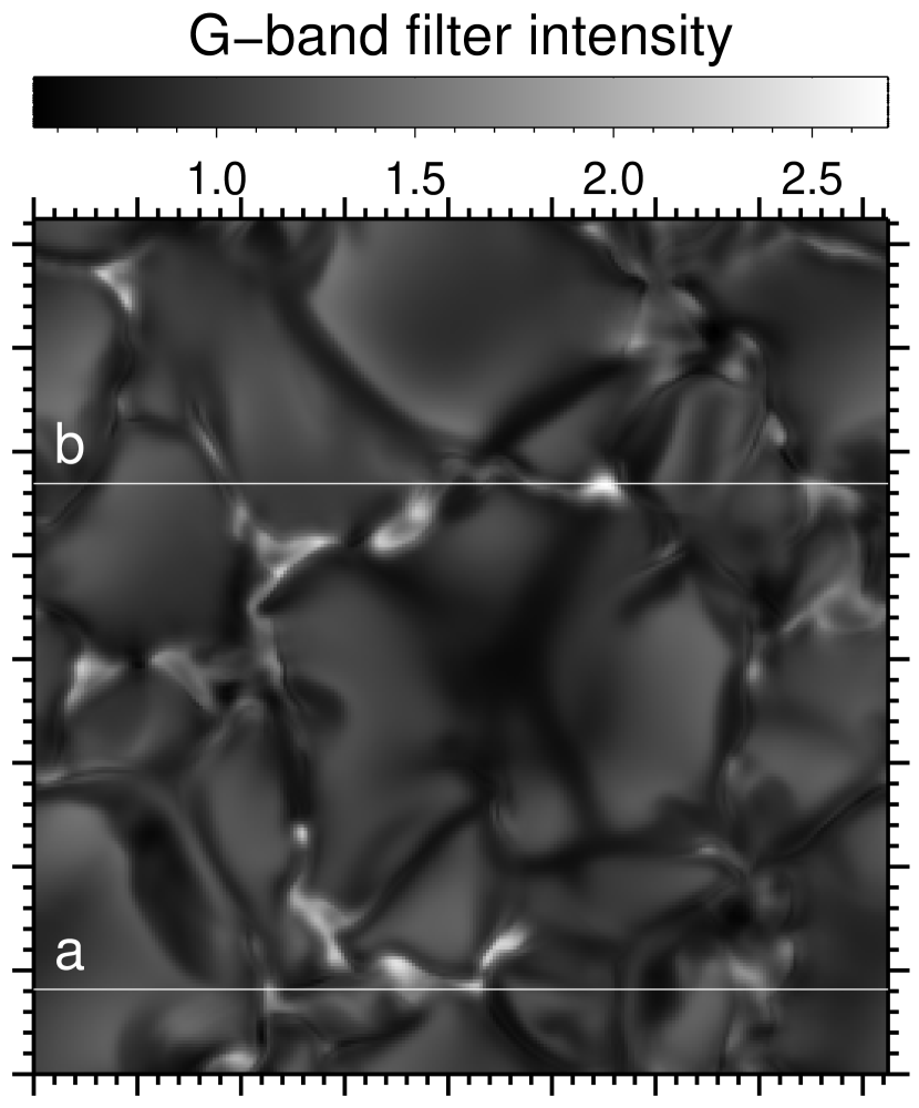
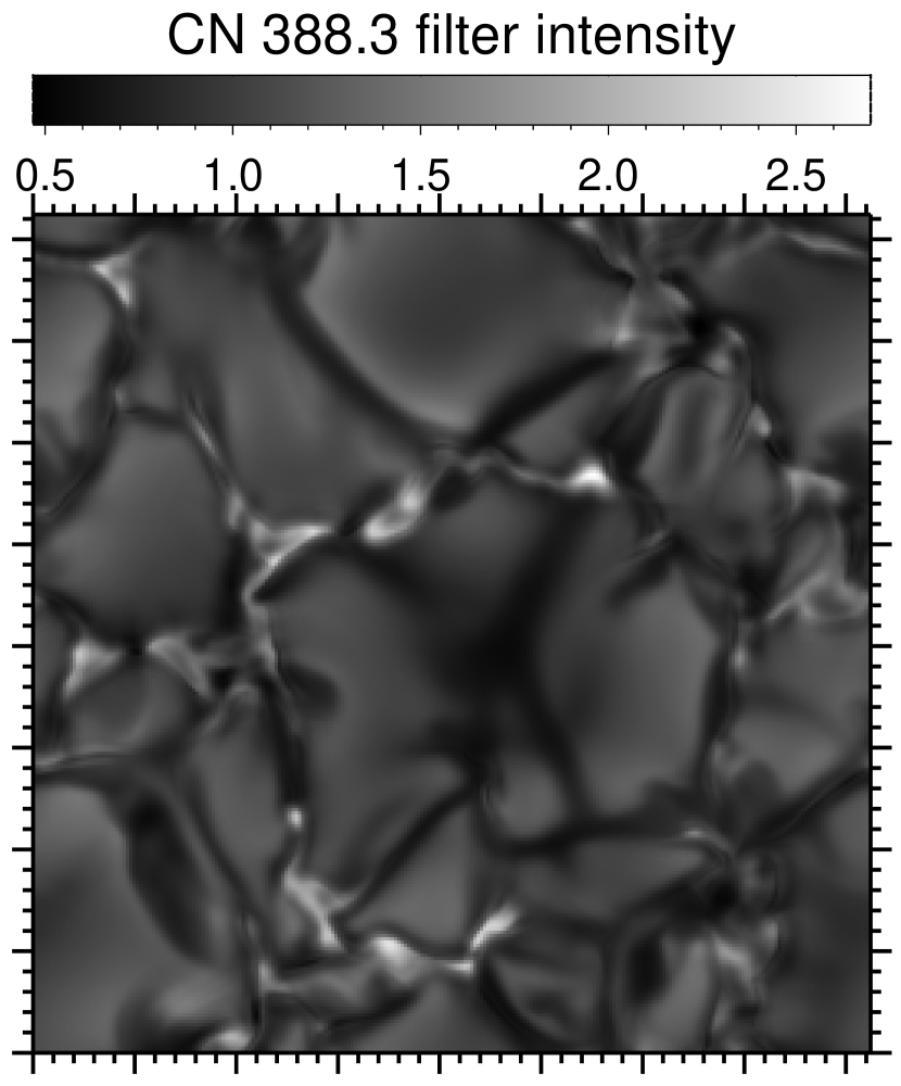
Figure 3: Synthetic filtergrams in the G band (left panel) and violet CN band constructed from the calculated disk-centre spectra. The intensity in each filtergram is normalised with respect to the average quiet-Sun value for that band. Major tick marks correspond to one arcsec intervals. Horizontal lines $a$ and $b$ mark cross sections used in Figures 4 and 7.

The RMS contrast over the whole field-of-view (FOV) is 22.0 % and 20.5,% for the CN band and the G band, respectively. The larger contrast in the CN band is the result of its shorter wavelength, but the difference is much smaller than expected on the basis of consideration of the temperature sensitivity of the Planck function. A convenient measure to express the difference in temperature sensitivity of the Planck fuction $B_{\lambda}(T)$ between the two wavelengths of the molecular bands is the ratio

$$\frac{B_{388.3}(T)}{B_{388.3}(4500)}/\frac{B_{430.5}(T)}{B_{430.5}(4500)},$$ (2)

where $T=4500$ is the average temperature of the photosphere at $z=0$. Since characteristic temperature differences between granules and intergranular lanes are 4000 K at this height we would expect a much higher value for the ratio of the granular contrast bewteen the CN and the CH band (eq. [2] gives 1.26 for $T=6500$, and 1.45 for $T=8500$) than the one we find in the present filtergrams. However, three circumstances reduce the contrast in the 388.3 nm filter signal with respect to that in the 430.5 nm band. First, the filter averages over lines and continuum wavelengths and at the formation height of the lines the temperature fluctuations are much smaller (e.g., at $z=150$ km the temperature differences are typically only 800 K). Secondly, because of the strong temperature sensitivity of the H^- opacity, optical depth unity contours (which provide a rough estimate of the formation height, see also Sect. 3) approximately follow temperature contours and thus sample much smaller temperature variations horizontally than they would at a fixed geometrical height. Finally, the CN concentration is reduced in the intergranular lanes (see Figure 1) with respect to the CH concentration. This causes weakening of the CN lines and raises the filter signal in the lanes, thereby preferentially reducing the contrast in the CN filtergram compared to values expected from Planck function considerations.

3 Filter Response functions

We use response functions to examine the sensitivity of the filter integrated signals to temperature at different heights in the solar atmosphere. The concept of response functions was first explored by Beckers & Milkey (1975) and further developed by Landi Deglinnocenti & Landi Deglinnocenti (1977) who generalised the formalism to magnetic lines, and also put forward the line integrated response function (LIRF) in the context of broad-band measurements. We derive the temperature response function in the inhomogeneous atmosphere by numerically evaluating the changes in the CH and CN filter integrated intensities that results from temperature perturbations introduced at different heights in the atmosphere. Since it is numerically very intensive the computation is performed only on a two-dimensional vertical cross-section through the three-dimensional magnetoconvection snapshot, rather than on the full cube. Our approach is very similar to the one used by Fossum & Carlsson (2005) to evaluate the temperature sensitivity of the signal observed through the 160 nm and 170 nm filters of the TRACE instrument.

Given a model of the solar atmosphere we can calculate the emergent intensity $I_{\lambda}$ and fold this spectrum through filter function $F_{\lambda}$ to obtain the filter integrated intensity

$$f=\int_{0}^{\infty}I_{\lambda}F_{\lambda}d\lambda.$$ (3)

Let us define the response function $R^{f,T}_{\lambda}(h)$ of the filter-integrated emergent intensity to changes in temperature $T$ by:

$$f\equiv\int_{-\infty}^{z_{0}}R^{f,T}_{\lambda}(z)T(z)dz,$$ (4)

where $z$ is the height in the semi-infinite atmosphere and $z_{0}$ marks its topmost layer. Written in this way the filter signal $f$ is a mean representation of temperature $T$ in the atmosphere weighted by the response function $R$. If we now perturb the temperature in different layers in the atmosphere and recalculate the filter-integrated intensity we obtain a measure of the sensitivity of the filter signal to temperature at different heights. More specifically, if we introduce a temperature perturbation of the form (Fossum & Carlsson, 2005)

$$\Delta T(z^{\prime})=t(z^{\prime})H(z^{\prime}-z),$$ (5)

where $H$ is a step function that is 0 above height $z$ and 1 below, the resulting change in the filter-integrated intensity is formally given by:

$$\Delta f_{z}=\int_{-\infty}^{z}R^{f,T}(z^{\prime})t(z^{\prime})dz^{\prime}.$$ (6)

Subsequently applying this perturbation at each height $z$ in the numerical grid, recalculating $f$, and subtracting the result from the unperturbed filter signal yields a function $\Delta f_{z}$ which can be differentiated numerically with respect to $z$ to recover the response function:

$$R^{f,T}(z)=\frac{1}{t(z)}\frac{d}{dz}\left(\Delta f_{z}\right).$$ (7)

To evaluate the response functions presented here we used perturbation amplitudes of 1% of the local temperature, i.e. $t(z)=0.01\quad T(z)$. Note that we do not adjust the density and ionization equilibria in the atmosphere when the temperature is perturbed, so that the perturbed models are not necessarily physically consistent. However, since we only introduce small perturbations, the resulting error in the estimate of the response function is expected to be small.

Figure 4 illustrates the behaviour of the G-band (bottom panel) and CN band head (top panel) filter response functions $R^{f,T}$ in the inhomogeneous magnetoconvection dominated atmosphere. It shows the depth-dependent response function for the two filter intensities in the vertical slice through the simulation snapshot marked by $a$ in the G-band panel in Figure 3. This cut intersects four G-band (and CN band) bright points at $x=2.2,3.6,4.2$, and 7.0 arcsec, the location of which is marked by the vertical dotted lines in the bottom panel. The solid and dashed curves mark the location of optical depth $\tau_{l}=1$ in the vertical line-of sight in a representative CN and CH line core, and optical depth $\tau_{c}=1$ in the continuum in each of the two wavelength intervals, respectively. The dash-dotted curve in the top panel marks optical depth $\tau_{h}=1$ in the CN band head at 388.339 nm.

The response functions have their maximum for each position along the slice just below the location of optical depth unity in the continuum at that location, indicating that the filter intensity is most sensitive to temperature variations in this layer. At each $x$ location the response functions show an upward extension up to just below the $\tau_{l}=1$ curves. This is the contribution of the multitude of molecular and atomic lines to the temperature sensitivity of the filter signals. We note that both the CN and CH filter response functions are very similar in shape, vertical location, and extent, with a slightly larger contribution of line over continuum in the case of the G band, which is related to the larger number densities of CH (see Figure 1). The highest temperature sensitivity results from the large continuum contribution over the tops of the granules. This is where the temperature gradient is steepest and the lines are relatively deep as evidenced by the larger height difference between the $\tau_{c}=1$ and $\tau_{l}=1$ curves (given the assumption of LTE intensity formation and an upward decreasing temperature). In the intergranular lanes the temperature gradient is much shallower, resulting in a lower sensitivity of the filter signal to temperature. This is particularly clear at $x=6$ arcsec, but also in the lanes just outside strong magnetic field configurations at $x=2.5$, and 4.4 arcsec.

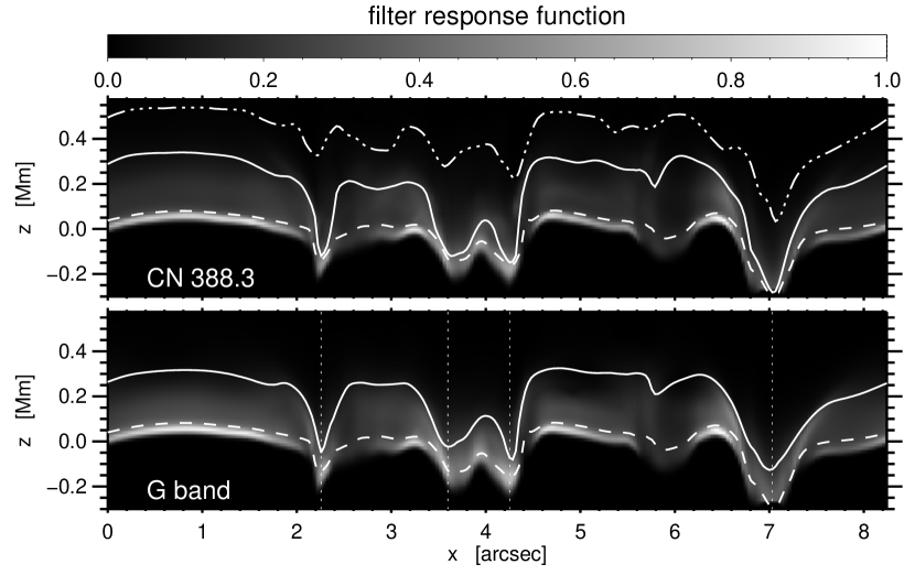
Figure 4: Response functions to temperature for the G-band (bottom) and CN-band filter signals in the two-dimensional vertical cross section marked $a$ in Figure 3. Dashed and solid curves mark vertical optical depth unity in the continuum and a typical molecular line ($\lambda=387.971$ nm for CN and $\lambda=430.390$ nm for CH), respectively. Optical depth unity of the CN band head at 388.339 nm is marked with the dash-dotted curve in the top panel. The locations of bright points in the cross section are indicated by the vertical dotted lines.

From the position of the vertical dotted lines marking the location of bright points in the filter intensity it is clear that these bright points result from considerable weakening of the CH and CN lines. At each of the bright point locations the $\tau_{l}=1$ curve dips down steeply along with the upward extension of the response function, bringing the formation heights of the line cores closer to those of the continuum, therefore weakening the line, and amplifying the wavelength integrated filter signal. This dip, which is the result of the partial evacuation of the magnetic elements, is more pronounced in the CN line-opacity because CN number densities decrease with depth in the flux concentration. (see Figure 1 and Section 2.1).

Remarkably, the CN band head proper with many overlapping lines has such a high opacity that it forms considerably higher than typical CN lines in the 388.3 nm interval (see the dash-dotted curve in the top panel in Figure 4). This means that its emergent intensity is less sensitive to the magnetic field presence because the field in the higher layers is less concentrated and, therefore, less evacuated, leading to a less pronounced dip in the optical depth $\tau_{h}=1$ curve. Narrow band filtergrams or spectroheliograms (e.g., Sheeley, 1971) that mostly cover the CN 388.3 nm band head can therefore be expected to have less contrast than filtergrams obtained through the 1 nm wide filters typically used in observations.

4 RMS intensity variation and bright-point contrast

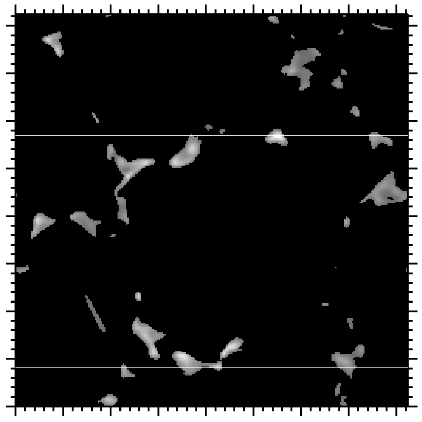
Figure 5: The G-band bright-point mask applied to the CH filtergram. The horizontal lines mark the same cross sections as in Figure 3.

We now turn to a comparison of the relative filter intensities and bright-point contrasts in the synthetic CH and CN band filtergrams. To study the properties of bright points in the two synthetic filtergrams we need to isolate them. In observations this can be done by subtracting a continuum image, in which the bright points have lower contrast but the granulation has similar contrast, from the molecular band image (Berger et al., 1998). We employ a similar technique here, but instead of using an image obtained through a broad-band filter centered on a region relatively devoid of lines, we use an image constructed from just one wavelength position, namely at $\lambda=430.405$ nm. More specifically, we count all pixels that satisfy

$$\frac{f_{\mathrm{G-Band}}}{<f_{\mathrm{G-Band}}>}-0.65\frac{I_{430.405}}{<I_{430.405}>}\quad\geq 0.625$$ (8)

as bright point pixels, where $f_{\mathrm{Gband}}$ is the G-band filtergram, $I_{430.405}$ the continuum image, and averaging is performed over the whole FOV. The value 0.65 was chosen to optimally eliminate granular contrast in the difference image, while the limit 0.625 was chosen so that only pixels with a relative intensity larger than 1.0 were selected. Furthermore, we define the average quiet-Sun intensity $<f>_{QS}$ as the average of $f$ over all pixels that form the complement mask of the bright-point mask. The resulting bright-point mask is shown in Figure 5 applied to the G-band filtergram.

Table 2: RMS intensity variation and average bright-point contrast in the synthetic CH and CN filtergrams.

Filter	RMS intensity	BP contrast
G-band	20.5%	0.497
CN	22.0%	0.478
CN (Zakharov)	19.7%	0.413
CN (SST)	23.6%	0.461

Defining the contrast of a pixel as

$$C=f/<f>_{QS}-1,$$ (9)

the bright point mask is used to compute the contrast of bright points in the CH and CN filtergrams for the different filters listed in Table 1. The results are presented in Table 2 along with the RMS intensity variation over the whole FOV. The synthetic filtergram CN filter centered at 388.3 nm yields an average bright-point contrast of 0.478, very close to the value of 0.481 reported by Zakharov et al. (2005, their table 1). We find an average bright point contrast for the CH filter of $<C_{\mathrm{CH}}>=0.497$, which is much higher than the experimental value of 0.340 reported by these authors. Averaged over all the bright points defined in Eq. [8] we find a contrast ratio of $<C_{\mathrm{CN}}>/<C_{\mathrm{CH}}>=0.96$, in sharp contrast to the observed value of 1.4 quoted by Zakharov et al. (2005). Using their filter parameters, moreover, we find an even lower theoretical value of $<C_{\mathrm{CN}}>=0.413$, and a contrast ratio of only 0.83.

This variation of bright-point contrast in the CN filter filtergrams with the central wavelength of the filter is caused by the difference in the lines that are covered by the filter passband. In the case of the La Palma filter and the Zakharov filter in particular, the filter band integrates over several strong atomic lines, which are less susceptible to line weakening than the molecular lines, and therefore contribute less to the contrast enhancement of magnetic elements (see Figure 8 in the next section).

Figure 6: Scatter plot of the CH and CN band contrasts of bright-point pixels versus relative intensity in the CH filtergram.

Figure 6 shows the scatter in the ratio of CH over CN contrast for all individual bright-point pixels. At low CH intensity values of $f/<f>_{QS}<1.3$ the CH contrast is much larger than the contrast in the CN filtergram. Above this value the contrast in CH and CN is on average very similar with differences becoming smaller towards the brightest points. Note that the scatter of the contrast ratio in CH and CN is not dissimilar to the one presented by Zakharov et al. (2005, their figure 4) except that the label on their ordinate contradicts the conclusion in their paper and appears to have the contrast ratio reversed.

Figure 7: Relative intensities of the CH (solid curves) and CN (dashed curves) filter images in two cross sections of the simulation snapshot indicated by the horizontal lines in the left panel of Figure 3 (bottom panel corresponds to cross section $a$, the same cross section was used for the response function in Figure 4), to panel corresponds to $b$.

To better display the difference in contrast between the two filtergrams we plot their values in two cross sections indicated by the horizontal lines in the left panel of Figure 3 in Figure 7. The contrast is clearly higher in granules and lower in intergranular lanes in the CN image, but is identical in the bright points (at $x=2.2$, 3.6, 4.2, and 7.0 arcsec in the left panel, and at $x=3.8$, 5.6, and 7.6 arcsec in the right panel, see also Figure 5). The lower contrast in the lanes and higher contrast in the granules in CN is caused by the higher sensitivity of the Planck function at the shorter wavelength of the CN band head when compared to the G band.

5 Discussion

In the synthetic CH- and CN-band filtergrams we find an average bright-point contrast ratio $<C_{\mathrm{CN}}>/<C_{\mathrm{CH}}>=0.96$ which is very different from the observational value of 1.4 reported by Zakharov et al. (2005). If we employ the parameters of the CN filter specified by these authors with a central wavelength of 388.7 nm, redward of the CN band head, we find an even lower theoretical contrast ratio 0.83. Previously, several authors (Rutten et al., 2001; Berdyugina et al., 2003) have predicted, on the basis of semi-empirical fluxtube modeling, that bright points would have higher contrast in the CN-band with contrast ratio values in line with the observational results of Zakharov et al. (2005). In these semi-empirical models it is assumed that flux elements can be represented by either a radiative equilibrium atmosphere of higher effective temperature, or a hot fluxtube atmosphere with a semi-empirically determined temperature stratification, in which case the stronger non-linear dependence of the Planck function at short wavelengths results in higher contrast in the CN band. Indeed if we use the same spectral synthesis data as for the three-dimensional snapshot, and define the ratio of contrasts in the CN band over the CH Band as

$$R=\frac{f_{\mathrm{CN}}(T_{\mathrm{eff}})/f_{\mathrm{CN}}(5750)-1.0}{f_{\mathrm{CH}}(T_{\mathrm{eff}})/f_{\mathrm{CH}}(5750)-1.0},$$ (10)

where $f(T_{\mathrm{eff}})$ is the filter signal for a Kurucz model with effective temperature $T_{\mathrm{eff}}$, we find that $R$ increases to 1.35 for $T_{\mathrm{eff}}=6250$ and then decreases again slightly for higher effective temperatures because the CN lines weaken more than the CH lines (see also Berdyugina et al., 2003).

However, more recent modeling, using magnetoconvection simulations like the one employed here has shown that magnetic elements derive their enhanced contrast from the partial evacuation in high field concentrations, rather than from temperature enhancement (Uitenbroek, 2003; Keller et al., 2004; Carlsson et al., 2004). Here we make plausible that the close ratio of bright-point contrast in CN and CH filtergrams we find in the synthetic images is consistent with this mechanism of enhancement through evacuation.

Figure 8: Short sections of G-band (bottom) and CN band (top) spectra for a typical granule (thick solid curve), bright point (thick dashed), and the spatial average (thin solid). Vertical lines at the top mark positions of CH and CN lines in the two intervals, respectively.

Analysis of the filter response function to temperature, and the behavior of the formation height of lines and the continuum in the CN- and CH-band as traced by the curves of optical depth unity (see Figure 4) already indicate that the evacuation of magnetic elements plays an important role in the appearance of these structures in the filtergrams. This is even more evident in the short sections of spectra plotted in Figure 8, which show the average emergent intensity over the whole snapshot (thin solid curve), and the intensity from a bright point (thick dashed curve) and a granule (thick solid curve) on an absolute intensity scale. Comparing the granular spectrum with that of the bright-point we notice that their continuum values are almost equal but that the line cores of molecular lines have greatly reduced central intensities in the bright point, which explains why the magnetic structures can become much brighter than granules in the CN and CH filtergrams. If the high intensity of bright points in the filtergrams would arise from a comparatively higher temperature, also their continuum intensities would be higher than in granules. Observational evidence for weakening of the line-core intensity in G-band bright points without brightening of the continuum is provided by Langhans et al. (2001, 2002).

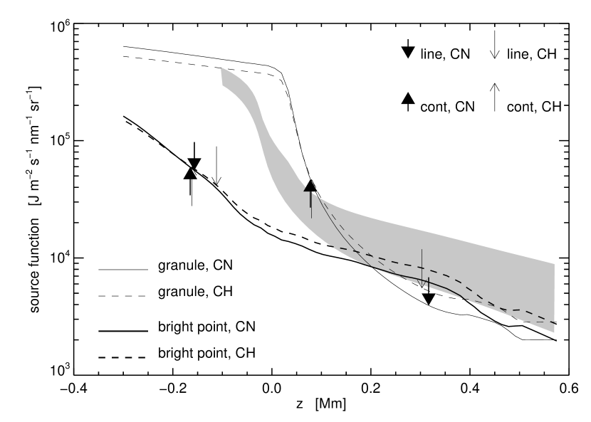
Figure 9: Source function of typical granule (thin curves) and bright point (thick curves) for the CH (dashed) and CN band (solid). Upward arrows mark the location of optical depth unity for continuum wavelengths, downward arrows that for line-center wavelengths. The shaded area marks the region between the Planck functions for solar Kurucz models of effective temperature 5750 K and 6750 K.

Line weakening in Figure 8 is less pronounced in the CN band head at 388.339 nm because the overlap of many lines raises the formation height to higher layers where the density is less affected by evacuation (see Sect. 3). Also atomic lines are less affected by the evacuation than lines of the CN and CH molecule (e.g., compare the lines at $\lambda=430.252$ nm and 430.320 nm with the weakened CH lines in the bottom panel of Figure 8), because the concentration the atomic species is only linearly dependent on density, while that of diatomic molecules is proportional to the square of the density of their constituent atoms. The latter effect is clear in the reduced number densities of CN and CH in bright points compared to intergranular lanes as shown in Figure 1 (see Section 2.1).

The partially evacuated magnetic concentrations are cooler than their surroundings in a given geometric layer. Radiation however, escapes both regions from similar temperatures, at necessarily different depths. This is made clear in Figure 9, which shows the source function (i.e., the Planck function, since we assume LTE) in the CH and CN bands for the location of the same granule and bright point for which the spectra in Figure 8 are drawn. The upward arrows mark the location of optical depth unity in the local continua, and the downward arrows mark the same for typical CN and CH lines in the bands. Both continuum and the CN and CH line centers in the bright point form approximately 250 km below the continuum in the granule, and they form very close together in both bands, resulting in pronounced weakening of the molecular lines. The structure of the response function (Figure 4) indicates that the continuum contributes dominantly to the temperature sensitivity of the filter integrated signals. It forms almost at the same temperature in the bright point and granule, hence the comparable continuum intensities in Figure 8, and the comparable brightness of granules and magnetic elements in continuum images. It is precisely for this reason that the bright-point contrast in the synthetic CN filtergram is very similar to that in CH, instead of being much higher. The high contrast of magnetic concentrations in these filtergrams results from line weakening in the filter passband, and not from temperatures that are higher than in a typical granule at the respective formation heights of the filter integrated signal.

The shaded region in Figure 9 indicates the range between Planck functions for solar Kurucz models (Kurucz, 1993a) of effective temperatures between 5750 K (bottom) and 6750 K (top) at the central wavelength of the G band filter. The comparison with the granule and bright point source functions shows that neither can be represented by a radiative equilibrium model, except near the top, where the mechanical flux in the simulations vanishes, and where the temperature in both structures converges towards the temperature in the standard solar model of $T_{\mathrm{eff}}=5750$ K. In particular, the temperature gradient in the flux element is much more shallow as the result of a horizontal influx of radiation from the hotter (at equal geometric height) surroundings. This shallow gradient further contributes to the weakening of the molecular spectral lines.

6 Conclusions

We have compared the brightness contrast of magnetic flux concentrations between synthesised filtergrams in the G-band and in the violet CN band at 388.3 nm, and find that, averaged over all bright points in the magnetoconvection simulation, the contrast in the CN band is lower by a factor of 0.96. This is in strong contradiction to the observational result reported by Zakharov et al. (2005), who find that the bright-point contrast is typically 1.4 times higher in CN-band filtergrams. In the present simulation the enhancement of intensity in magnetic elements over that of quiet-Sun features is caused by molecular spectral line weakening in the partially evacuated flux concentration. At the median formation height of the filter intensity (as derived from the filter’s temperature response function, Figure 4) the temperature in the flux concentration is comparable to that of a typical granule (Figure 9). As a result of these two conditions the contrast between the bright point intensity and that of the average quiet-Sun is very similar in both the CH and CN filters, and not higher in the latter as would be expected from Planck function considerations if the enhanced bright point intensity were the result of a higher temperature in the flux concentration at the filter intensity formation height.

The ratio of CH bright point contrast over that of the CN band varies with bright point intensity (Figure 6), with a relatively higher G-band contrast for fainter elements. Theoretically, this makes the G band slightly more suitable for observing these lower intensity bright points.

Because the bright-point contrast in filtergrams is the result of weakening of the molecular lines in the filter passband its value depends on the exact position and width of the filter (see Table 2). The transmission band of the filter used by Zakharov et al. (2005) mostly covers atomic lines of neutral iron and the hydrogen Balmer H₈ line, and hardly any CN lines because it was centered redward of the band head at 388.339 nm. Hence the theoretical contrast obtained with this filter is even lower than with the nominal filter centered at the band head.

We find that the RMS intensity variation in the CN filtergram is slightly higher than in the CH dominated G band with values of 22.0 % and 20.5 %, respectively. The former value depends rather strongly on the central wavelength of the employed filter (Table 2). The greater intensity variation in the CN-band filtergram is the result of the stronger temperature sensitivity of the Planck function at 388.3 nm than at 430.5 nm. These intensity variations are moderated by the fact that the filter integrates over line and continuum wavelengths combined with a decrease in horizontal temperature variation with height, the strong opacity dependence of the H^- opacity, and the strong decrease of the CN number density with temperature and depth in the intergranular lanes (Section 2.1). The low RMS intensity variation through the filter described by Zakharov et al. (2005) is the result of the inclusion of the hydrogen H₈ line in the passband. Similarly to the H$\alpha$ line the reduced contrast in the H₈ line is the result of the large excitation energy of its lower level, which makes the line opacity very sensitive to temperature (Leenaarts et al., 2005). A positive temperature perturbation will strongly increase the hydrogen $n_{2}$ number density (through additional excitation in Ly$\alpha$) forcing the line to form higher at lower temperature thereby reducing the intensity variation in the line, and vice versa for a negative perturbation.

Finally, the mean spectrum, averaged over the area of the simulation snapshot, closely matches the observed mean disk-center intensity (Figure 2), providing confidence in the realism of the underlying magnetoconvection simulation and our numerical radiative transfer modeling. Moreover, the filter integrated quantities we compare here are not very sensitive to the detailed shapes of individual spectral lines (for instance, the filter contrasts are the same with a carbon abundance $\epsilon_{C}=8.60$, although the CN lines in particular provide a much less accurate fit to the mean observed spectrum in that case). The clear discrepancy between the observed and synthetic contrasts, therefore, indicates that we lack complete understanding of either the modeling, or the observations, including the intricacies of image reconstruction at two different wavelengths at high resolution, or both. In particular, the near equality of bright point contrast in the two CN and CH bands is a definite signature of brightening through evacuation and the concomitant line weakening. If observational evidence points to a clear wavelength dependence of the bright point contrast, it may indicate that the simulations lack an adequate heating mechanism in their magnetic elements.

References

- Asensio Ramos et al. (2003) Asensio Ramos, A., Trujillo Bueno, J., Carlsson, M., & Cernicharo, J. 2003, ApJ, 588, L61
- Asplund et al. (2005) Asplund, M., Grevesse, N., Sauval, A. J., Allende Prieto, C., & Blomme, R. 2005, A&A, 431, 693
- Asplund et al. (2004) Asplund, M., Grevesse, N., Sauval, A. J., Allende Prieto, C., & Kiselman, D. 2004, A&A, 417, 751
- Beckers & Milkey (1975) Beckers, J. M., & Milkey, R. W. 1975, Sol. Phys., 43, 289
- Berdyugina et al. (2003) Berdyugina, S. V., Solanki, S. K., & Frutiger, C. 2003, A&A, 412, 513
- Berger et al. (1998) Berger, T. E., Löfdahl, M. G., Shine, R. S., & Title, A. M. 1998, ApJ, 495, 973
- Berger et al. (1995) Berger, T. E., Schrijver, C. J., Shine, R. A., Tarbell, T. D., Title, A. M., & Scharmer, G. 1995, ApJ, 454, 531
- Berger & Title (2001) Berger, T. E., & Title, A. M. 2001, ApJ, 553, 449
- Brault & Neckel (1987) Brault, J. W., & Neckel, H. 1987, Spectral Atlas of Solar Absolute Disk-averaged and Disk-center Intensity from 3290 to 12510 Å, available with anonymous FTP at ftp.hs.uni-hamburg.de/pub/outgoing/FTS-atlas
- Carlsson et al. (2004) Carlsson, M., Stein, R. F., Nordlund, Å., & Scharmer, G. B. 2004, ApJ, 610, L137
- Cox (2000) Cox, A. N. 2000, Allen’s astrophysical quantities, Allen’s astrophysical quantities, 4th ed. Publisher: New York: AIP Press; Springer, 2000. Editedy by Arthur N. Cox. ISBN: 0387987460
- Fossum & Carlsson (2005) Fossum, A., & Carlsson, M. 2005, ApJ, 625, 556
- Grevesse & Anders (1991) Grevesse, N., & Anders, E. 1991, in A. Cox, W. Livingston, M. Matthews (eds.), Solar interior and atmosphere., University of Arizona Press, Tucson, AZ, p. 1227
- Keller et al. (2004) Keller, C. U., Schüssler, M., Vögler, A., & Zakharov, V. 2004, ApJ, 607, L59
- Kunasz & Auer (1988) Kunasz, P. B., & Auer, L. H. 1988, J. Quant. Spec. Radiat. Transf., 39, 67
- Kurucz (1993a) Kurucz, R. L. 1993a, ATLAS9 Stellar Atmosphere Programs and 2 km/s grid. Kurucz CD-ROM No. 13. Cambridge, Mass.: Smithsonian Astrophysical Observatory, 1993., 13
- Kurucz (1993b) Kurucz, R. L. 1993b, SYNTHE Spectrum Synthesis Programs and Line Data. Kurucz CD-ROM No. 18. Cambridge, Mass.: Smithsonian Astrophysical Observatory, 1993., 18
- Landi Deglinnocenti & Landi Deglinnocenti (1977) Landi Deglinnocenti, E., & Landi Deglinnocenti, M. 1977, A&A, 56, 111
- Langhans et al. (2001) Langhans, K., Schmidt, W., Rimmele, T., & Sigwarth, M. 2001, in M. Sigwarth (ed.), Advanced Solar Polarimetry – Theory, Observation, and Instrumentation, ASP Conf. Ser., Vol. 236, The Astronomical Society of the Pacific, San Francisco, CA, p. 439
- Langhans et al. (2002) Langhans, K., Schmidt, W., & Tritschler, A. 2002, A&A, 394, 1069
- Leenaarts et al. (2005) Leenaarts, J., Sütterlin, P., Rutten, R. J., Carlsson, M., & Uitenbroek, H. 2005, A&A, submitted
- Mount & Linsky (1974a) Mount, G. H., & Linsky, J. L. 1974a, Sol. Phys., 35, 259
- Mount & Linsky (1974b) Mount, G. H., & Linsky, J. L. 1974b, Sol. Phys., 36, 287
- Mount & Linsky (1975a) Mount, G. H., & Linsky, J. L. 1975a, ApJ, 202, L51
- Mount & Linsky (1975b) Mount, G. H., & Linsky, J. L. 1975b, Sol. Phys., 41, 17
- Mount et al. (1973) Mount, G. H., Linsky, J. L., & Shine, R. A. 1973, Sol. Phys., 32, 13
- Muller et al. (1989) Muller, R., Hulot, J. C., & Roudier, T. 1989, Sol. Phys., 119, 229
- Muller & Roudier (1992) Muller, R., & Roudier, T. 1992, Sol. Phys., 141, 27
- Muller et al. (1994) Muller, R., Roudier, T., Vigneau, J., & Auffret, H. 1994, A&A, 283, 232
- Neckel (1999) Neckel, H. 1999, Sol. Phys., 184, 421
- Rutten et al. (2001) Rutten, R. J., Kiselman, D., Rouppe van der Voort, L., & Plez, B. 2001, in M. Sigwarth (ed.), Advanced Solar Polarimetry – Theory, Observation, and Instrumentation, ASP Conf. Ser., Vol. 236, The Astronomical Society of the Pacific, San Francisco, CA, p. 445
- Sauval & Tatum (1984) Sauval, A. J., & Tatum, J. B. 1984, ApJS, 56, 193
- Schüssler et al. (2003) Schüssler, M., Shelyag, S., Berdyugina, S., Vögler, A., & Solanki, S. K. 2003, ApJ, 597, L173
- Sheeley (1971) Sheeley, N. R. 1971, Sol. Phys., 20, 19
- Stein & Nordlund (1998) Stein, R. F., & Nordlund, Å. 1998, ApJ, 499, 914
- Uitenbroek (1998) Uitenbroek, H. 1998, ApJ, 498, 427
- Uitenbroek (2000a) Uitenbroek, H. 2000a, ApJ, 531, 571
- Uitenbroek (2000b) Uitenbroek, H. 2000b, ApJ, 536, 481
- Uitenbroek (2003) Uitenbroek, H. 2003, in A. A. Pevtsov, H. Uitenbroek (eds.), Current Theoretical Models and High Resolution Solar Observations: Preparing for ATST, ASP Conf. Ser., Vol. 286, The Astronomical Society of the Pacific, San Francisco, CA, p. 404
- van Ballegooijen et al. (1998) van Ballegooijen, A. A., Nisenson, P., Noyes, R. W., Löfdahl, M. G., Stein, R. F., Nordlund, Å., & Krishnakumar, V. 1998, ApJ, 509, 435
- Wedemeyer-Böhm et al. (2005) Wedemeyer-Böhm, S., Kamp, I., Bruls, J., & Freytag, B. 2005, A&A, 438, 1043
- Zakharov et al. (2005) Zakharov, V., Gandorfer, A., Solanki, S. K., & Löfdahl, M. 2005, A&A, 437, L43