Radio Astronomical Polarimetry and High-Precision Pulsar Timing

Abstract

A new method of matrix template matching is presented in the context of pulsar timing analysis. Pulse arrival times are typically measured using only the observed total intensity light curve. The new technique exploits the additional timing information available in the polarization of the pulsar signal by modeling the transformation between two polarized light curves in the Fourier domain. For a number of millisecond pulsars, arrival time estimates derived from polarimetric data are predicted to exhibit greater precision and accuracy than those derived from the total intensity alone. Furthermore, the transformation matrix produced during template matching may be used to calibrate observations of other point sources. Unpublished supplementary material is appended after the bibliography.

1 Introduction

High-precision pulsar timing is a well-established technique of modern astrophysics; it has yielded the strongest constraints on theories of gravitation in the strong-field regime (Stairs, 2004), and is anticipated to provide a direct detection of the stochastic gravitational wave background due to supermassive black hole binaries (Jenet et al., 2005). Fundamental to every pulsar timing experiment is a measurement known as the pulse time-of-arrival (TOA), the epoch at which a fiducial phase of the pulsar’s periodic signal is received at the observatory. The confidence limits of the various physical parameters that are derived from the TOA data depend upon the precision and accuracy with which arrival times can be estimated.

In addition to typical constraints such as the system temperature, instrumental bandwidth, and integration length, TOA precision also depends upon the physical properties of the observed pulsar, including its total flux density, pulse period, and the shape of its phase-resolved light curve, or pulse profile. When fully resolved, narrow features in the pulse profile provide strong constraints during template matching, thereby yielding greater arrival time precision (see § 3.2). The polarized component of the pulsar signal often displays much sharper features than observed in the total intensity, especially when the pulsar exhibits transitions between orthogonally polarized modes. This important property may be exploited to significantly improve timing precision by incorporating polarization data.

Pulsar polarization also impacts on timing accuracy (Cordes et al., 2004). The total intensity profile can be significantly distorted by instrumental artifacts, a problem most readily observed as a systematic variation of arrival time residuals with parallactic angle (van Straten, 2003). To address this issue, Britton (2000) proposed timing the polarimetric invariant profile, which greatly improved the timing accuracy of PSR J0437$-$4715 (Britton et al., 2000). However, there are disadvantages of using the invariant profile; its signal-to-noise ratio (S/N) is at most $1/\sqrt{2}$ times that of the total intensity (see § 4) and inversely proportional to the degree of polarization; also, its computation suffers from imprecision in the estimation of the off-pulse signal. Therefore, use of the invariant profile can be detrimental when the pulsar is highly polarized or has low flux density.

In contrast, the matrix template matching technique presented in this paper can be used to improve both the precision and accuracy of arrival time estimates without any sensitivity to mean off-pulse polarization. The method simultaneously yields the polarimetric transformation between the template and observed profiles, which may be utilized to completely calibrate the instrumental response in other observations. Following a review of the required mathematics in § 2, the matrix template matching technique is formulated and quantitatively compared with scalar methods in § 3. In § 4, the analysis is demonstrated using a sample of millisecond pulsars. The application of matrix template matching to instrumental calibration is outlined in § 5, and the main conclusions of this work are summarized in § 6.

2 Review of the Jones Calculus

The formulation and analysis of the matrix template matching method utilizes the terminology and notation reviewed in this section. The polarization of electromagnetic radiation is described by the second-order statistics of the transverse electric field vector, $e$, as represented using the complex $2\times 2$ coherency matrix, $\mbox{\boldmath$\rho$}=\langle\mbox{\boldmath$e\otimes e$}^{\dagger}\rangle$ (Born & Wolf, 1980). Here, the angular brackets denote an ensemble average, $\otimes$ is the matrix direct product, and $\mbox{\boldmath$e$}^{\dagger}$ is the Hermitian transpose of $e$. The coherency matrix is commonly expressed as a linear combination of Hermitian basis matrices, ${\mbox{\boldmath$\rho$}}=(S_{0}\,\mbox{\boldmath$\sigma$}_{0}+\mbox{\boldmath$S\cdot\sigma$})/2$, where $\mbox{\boldmath$\sigma$}_{0}$ is the $2\times 2$ identity matrix, $\mbox{\boldmath$\sigma$}=(\mbox{\boldmath$\sigma$}_{1},\mbox{\boldmath$\sigma$}_{2},\mbox{\boldmath$\sigma$}_{3})$ are the Pauli spin matrices, $S_{0}$ is the total intensity, and $\mbox{\boldmath$S$}=(S_{1},S_{2},S_{3})$ is the polarization vector (Britton, 2000). The Pauli matrices are traceless and satisfy $\mbox{\boldmath$\sigma$}_{i}^{2}=\mbox{\boldmath$\sigma$}_{0}$; therefore, $S_{k}={\rm tr}(\mbox{\boldmath$\sigma$}_{k}\mbox{\boldmath$\rho$})$, where ${\rm tr}$ is the matrix trace operator (Hamaker, 2000).

In the analysis of the reception of polarized radiation, the following conventions are used. The response of a single receptor is defined by the Jones vector, $r$, such that the voltage induced in the receptor by the incident electric field is given by the scalar product, $v=\mbox{\boldmath$r$}^{\dagger}\mbox{\boldmath$e$}$. A dual-receptor feed is represented by the Hermitian transpose of a Jones matrix with columns equal to the Jones vector of each receptor,

$${\bf J}=(\mbox{\boldmath$r$}_{0}\;\mbox{\boldmath$r$}_{1})^{\dagger}=\left(\begin{array}[]{cc}r_{00}^{*}&r_{01}^{*}\\ r_{10}^{*}&r_{11}^{*}\end{array}\right).$$ (1)

The receptors in an ideal feed respond to orthogonal senses of polarization (ie. the scalar product, $\mbox{\boldmath$r$}_{0}^{\dagger}\mbox{\boldmath$r$}_{1}=0$) and have identical gains (ie. $\mbox{\boldmath$r$}_{0}^{\dagger}\mbox{\boldmath$r$}_{0}=\mbox{\boldmath$r$}_{1}^{\dagger}\mbox{\boldmath$r$}_{1}$).

A more meaningful geometric interpretation of Jones vectors is provided by the corresponding Stokes parameters, $S_{k}={\rm tr}[\mbox{\boldmath$\sigma$}_{k}\mbox{\boldmath$r\otimes r$}^{\dagger}]$. The state of polarization to which a receptor maximally responds is completely described by the three components of its associated Stokes polarization vector, $S$. Therefore, it is common to define a receptor using the spherical coordinates of $S$ (Chandrasekhar, 1960); in the linear basis, these include the gain, $g=|\mbox{\boldmath$r$}|=|\mbox{\boldmath$S$}|^{1\over 2}$, the orientation,

$$\theta={1\over 2}\tan^{-1}{S_{2}\over S_{1}},$$ (2)

and the ellipticity,

$$\epsilon={1\over 2}\sin^{-1}{S_{3}\over|\mbox{\boldmath$S$}|},$$ (3)

such that

$$\mbox{\boldmath$r$}=g\left(\begin{array}[]{c}\cos\theta\cos\epsilon+i\sin\theta\sin\epsilon\\ \sin\theta\cos\epsilon-i\cos\theta\sin\epsilon\end{array}\right).$$ (4)

The impact of non-ideal feed receptors on pulsar timing is analyzed by exploiting a powerful classification of Jones matrices motivated by the polar decomposition. Any non-singular matrix can be decomposed into the product of a unitary matrix and a positive-definite Hermitian matrix. Using the axis-angle parameterization (Britton, 2000), the polar decomposition of a Jones matrix (Hamaker, 2000) is expressed as

$${\bf J}=J\,{\bf B}_{\mbox{\scriptsize\boldmath$\hat{m}$}}(\beta)\,{\bf R}_{\mbox{\scriptsize\boldmath$\hat{n}$}}(\phi),$$ (5)

where $J=(\det{\bf J})^{1\over 2}$, ${\bf B}_{\mbox{\scriptsize\boldmath$\hat{m}$}}(\beta)$ is positive-definite Hermitian, and ${\bf R}_{\mbox{\scriptsize\boldmath$\hat{n}$}}(\phi)$ is unitary; both ${\bf B}_{\mbox{\scriptsize\boldmath$\hat{m}$}}(\beta)$ and ${\bf R}_{\mbox{\scriptsize\boldmath$\hat{n}$}}(\phi)$ are unimodular. The unit 3-vectors, $\hat{m}$ and $\hat{n}$, correspond to axes of symmetry in the three-dimensional space of the Stokes polarization vector. Under the congruence transformation of the coherency matrix, the Hermitian matrices,

$${\bf B}_{\mbox{\scriptsize\boldmath$\hat{m}$}}(\beta)=\exp(\beta\,\mbox{\boldmath$\hat{m}\cdot\sigma$})=\mbox{\boldmath$\sigma$}_{0}\cosh\beta+\mbox{\boldmath$\hat{m}\cdot\sigma$}\sinh\beta,$$ (6)

effect a Lorentz boost of the Stokes 4-vector along the $\hat{m}$ axis by an impact parameter $2\beta$, such that the resulting total intensity, $S^{\prime}_{0}=S_{0}\cosh 2\beta+\mbox{\boldmath$S\cdot\hat{m}$}\sinh 2\beta$. Similarly, the unitary matrices,

$${\bf R}_{\mbox{\scriptsize\boldmath$\hat{n}$}}(\phi)=\exp(i\phi\,\mbox{\boldmath$\hat{n}\cdot\sigma$})=\mbox{\boldmath$\sigma$}_{0}\cos\phi+i\mbox{\boldmath$\hat{n}\cdot\sigma$}\sin\phi,$$ (7)

rotate the Stokes polarization vector about the $\hat{n}$ axis by an angle $2\phi$, leaving the total intensity unchanged. This parameterization enables the important distinction between polarimetric transformations that mix the total and polarized intensities (boosts) and those that effect a change of basis (rotations).

3 Matrix Template Matching

The primary purpose of this paper is the formal description of the matrix template matching technique and the quantitative comparison of its effectiveness with that of conventional scalar methods. The performance of a method of TOA measurement may be evaluated in terms of the precision and accuracy of the arrival time estimates that it produces. The analysis of TOA precision requires careful attention to the propagation of experimental error, as described in § 3.2. TOA accuracy depends upon the susceptibility of the technique to sources of systematic error. To quantitatively compare different methods, a simulation that spans the full range of potential artifacts is devised in § 3.3.

3.1 Description of Technique

A pulsar’s mean pulse profile is measured by integrating the observed flux density as a function of pulse phase. By averaging many pulse profiles, one with high S/N may be formed and used as a template against which the individual observations are matched. The best-fit phase shift derived by the template matching procedure is then used to compute the pulse TOA.

Taylor (1992) presents a method for modeling the phase shift between the template and observed total intensity profiles in the Fourier domain. In the current treatment, the scalar equation that relates two total intensity profiles is replaced by an analogous matrix equation, which is expressed using the Jones calculus. Let the coherency matrices, $\mbox{\boldmath$\rho$}^{\prime}(\phi_{n})$, represent the observed polarization as a function of discrete pulse phase, $\phi_{n}$, where $0\leq n<N$ and $N$ is the number of intervals into which the pulse period is evenly divided. Each observed polarization profile is related to the template, $\mbox{\boldmath$\rho$}_{0}(\phi_{n})$, by the matrix equation,

$$\mbox{\boldmath$\rho$}^{\prime}(\phi_{n})={\bf J}\mbox{\boldmath$\rho$}_{0}(\phi_{n}-\varphi){\bf J}^{\dagger}+\mbox{\boldmath$\rho$}_{\mathrm{D}C}+\mbox{\boldmath$\rho$}_{\mathrm{N}}(\phi_{n}),$$ (8)

where ${\bf J}$ is the polarimetric transformation, $\varphi$ is the phase shift, $\mbox{\boldmath$\rho$}_{\mathrm{D}C}$ is the DC offset between the two profiles, and $\mbox{\boldmath$\rho$}_{\mathrm{N}}$ represents the system noise. The discrete Fourier transform (DFT) of equation (8) is

$$\mbox{\boldmath$\rho$}^{\prime}(\nu_{m})={\bf J}\mbox{\boldmath$\rho$}_{0}(\nu_{m}){\bf J}^{\dagger}\exp(-i2\pi\nu_{m}\varphi)+\mbox{\boldmath$\rho$}_{\mathrm{N}}(\nu_{m}),$$ (9)

where $\nu_{m}$ is the discrete frequency. Given the observed Stokes parameters, $S_{k}^{\prime}(\phi_{n})$, and their DFTs, $S_{k}^{\prime}(\nu_{m})$, the best-fit model parameters will minimize the objective merit function,

$$\chi^{2}=\sum_{m=1}^{N/2}\sum_{k=0}^{3}{|S_{k}^{\prime}(\nu_{m})-{\rm tr}[\mbox{\boldmath$\sigma$}_{k}\;\mbox{\boldmath$\rho$}^{\prime}(\nu_{m})]|^{2}\varsigma_{k}^{-2}},$$ (10)

where $\varsigma_{k}$ is equal to the rms of the noise in each DFT and ${\rm tr}$ is the matrix trace operator. As in van Straten (2004), the partial derivatives of equation (10) are computed with respect to both $\varphi$ and the seven non-degenerate parameters that determine ${\bf J}$. The Levenberg-Marquardt method is then applied to find the parameters that minimize $\chi^{2}$ (Press et al., 1992).

3.2 Timing Precision

When compared with the scalar technique, matrix template matching quadruples the number of observational constraints while introducing only six degrees of freedom. Therefore, arrival time estimates derived from the polarization profile might be expected to have greater precision than those derived from the total intensity profile alone. However, the effectiveness of matrix template matching depends upon both the degree of polarization and the variability of the polarization vector as a function of pulse phase. These properties determine the extent to which the phase shift, $\varphi$, is correlated with the free parameters that determine the Jones matrix, J.

To estimate the timing precision attainable by matrix template matching, consider the solution of equation (8) in the special case that J is known. After calibration, the minimization of equation (10) by variation of $\varphi$ requires finding the appropriate root of

$${\partial\chi^{2}\over\partial\varphi}=4\pi\sum_{m=1}^{N/2}\sum_{k=0}^{3}{|S_{k,m}|\over\varsigma_{k}^{2}}\nu_{m}\sin(\phi_{k,m}-2\pi\varphi\nu_{m}),$$ (11)

where $S_{k,m}=S_{k}^{\prime*}(\nu_{m}){\rm tr}[\mbox{\boldmath$\sigma$}_{k}\;\mbox{\boldmath$\rho$}_{0}(\nu_{m})]$ is the cross-spectral power of the template and observation and $\phi_{k,m}$ is the argument of $S_{k,m}$. To first order,

$${\partial\chi^{2}\over\partial\varphi}\simeq 4\pi\sum_{m=1}^{N/2}\sum_{k=0}^{3}{|S_{k,m}|\over\varsigma_{k}^{2}}(\phi_{k,m}\nu_{m}-2\pi\varphi\nu_{m}^{2})=0,$$ (12)

which is equivalent to the solution of a line with slope $2\pi\varphi$ passing through the origin and the points, $(\nu_{m},\phi_{k,m})$. This linear approximation is readily solved for $\varphi$ and used to determine the conditional variance,

$${\rm var}(\varphi|{\bf J})=\left[4\pi^{2}\sum_{m=1}^{N/2}\nu_{m}^{2}\sum_{k=0}^{3}{|S_{k,m}|\over\varsigma_{k}^{2}}\right]^{-1}.$$ (13)

Equation 13 demonstrates that fluctuation power contributes quadratically as a function of frequency to the reduction of the phase shift variance. In other words, sharper features in the pulse profile, which generate more power at higher harmonics, yield greater arrival time precision. This general results holds for both matrix and scalar template matching (in the scalar case, the sum over index $k$ stops at 0).

Equation 13 also provides an upper limit on the arrival time precision that may be obtained in the ideal case of a perfectly calibrated instrument. However, the instrumental response is generally unknown, and the Jones matrix must also be varied in order to minimize equation (10). The covariances between the phase shift, $\varphi$, and the free parameters that describe J will increase the uncertainty in $\varphi$ and therefore decrease arrival time precision.

Formally, the variance of $\varphi$ is determined by the covariance matrix of the free parameters, ${\bf C}={\mbox{\boldmath$\alpha$}}^{-1}$, where $\alpha$ is the curvature matrix. Assuming that the noise power in the DFT of each Stokes parameter is equal,

$$\alpha_{rs}={1\over 2}{\partial^{2}\chi^{2}\over\partial\eta_{r}\partial\eta_{s}}={2\over\varsigma^{2}}\sum_{m=1}^{N/2}{\rm Re}\left[{\rm tr}\left({\partial\mbox{\boldmath$\rho$}^{\prime\dagger}_{m}\over\partial\eta_{r}}{\partial\mbox{\boldmath$\rho$}^{\prime}_{m}\over\partial\eta_{s}}\right)\right].$$ (14)

If the free parameters, $\eta$, are partitioned into $\varphi=\eta_{0}$ and the seven Jones matrix parameters, $\mbox{\boldmath$\eta$}_{\bf J}$, then C may be conformably partitioned into (Stuart, Ord, & Arnold, 1999)

$${\bf C}=\left(\begin{array}[]{cc}c_{\varphi\varphi}&{\mbox{\boldmath$C$}}_{\varphi{\bf J}}^{T}\\ {\mbox{\boldmath$C$}}_{\varphi{\bf J}}&{\bf C_{JJ}}\end{array}\right),$$ (15)

and ${\rm var}(\varphi)=c_{\varphi\varphi}$. Furthermore, if the free parameters are multinormally distributed, then the multiple correlation between $\varphi$ and $\mbox{\boldmath$\eta$}_{\bf J}$,

$$R_{\varphi{\bf J}}=\left[c_{\varphi\varphi}^{-1}{\mbox{\boldmath$C$}}_{\varphi{\bf J}}^{T}{\bf C_{JJ}}^{-1}{\mbox{\boldmath$C$}}_{\varphi{\bf J}}\right]^{1\over 2},$$ (16)

describes the relationship between the variance and conditional variance of $\varphi$,

$${\rm var}(\varphi|{\bf J})={\rm var}(\varphi)(1-R^{2}_{\varphi{\bf J}}).$$ (17)

The multiple correlation coefficient, $0\leq R_{\varphi{\bf J}}\leq 1$, provides a useful measure of the decrease in arrival time precision that results from an unknown instrumental response. It is important to note that $R_{\varphi{\bf J}}$ can be computed using only the template polarization profile; that is, though $\alpha$ depends on $\mbox{\boldmath$\rho$}^{\prime}_{m}$ and $\varsigma$, all factors of $\varsigma$ are canceled in equation (16). Therefore, $R_{\varphi{\bf J}}$ is unique to each pulsar and is independent of the S/N of the observations.

However, the precision and accuracy with which $R_{\varphi{\bf J}}$ can be estimated does depend on the S/N of the template. In fact, measurement noise in the template polarization profile artificially decreases both the multiple correlation and the conditional variance of $\varphi$. To minimize the impact of noise on the computation of ${\rm var}(\varphi|{\bf J})$, $R_{\varphi{\bf J}}$, and ${\rm var}(\varphi)$, the summations over the index $m$ in equations (13) and (14) are performed up to a maximum harmonic, $M$, the highest frequency at which the fluctuation power spectra exhibit three consecutive harmonics with power greater than three times the mean noise power.

To completely eliminate the dependence on $\varsigma$, ${\rm var}(\varphi|{\bf J})$ and ${\rm var}(\varphi)$ are normalized by the corresponding variance in the phase shift, $\bar{\varphi}$, yielded by the conventional method of scalar template matching the total intensity profile. That is, equation (13) is used to predict the relative conditional timing error in the case of a known instrumental response,

$$\hat{\sigma}_{\varphi|{\bf J}}=\left[{{\rm var}(\varphi|{\bf J})\over{\rm var}(\bar{\varphi}|G)}\right]^{1\over 2}=\left[{\Sigma_{0}\over\Sigma_{0}+\Sigma_{1-3}}\right]^{1\over 2},$$ (18)

where $G$ is the absolute gain,

$$\Sigma_{0}=\sum_{m=1}^{M}\nu_{m}^{2}|S_{0}(\nu_{m})|^{2}$$ (19)

and

$$\Sigma_{1-3}=\sum_{m=1}^{M}\nu_{m}^{2}|\mbox{\boldmath$S$}(\nu_{m})|^{2}.$$ (20)

Similarly,

$$\hat{\sigma}_{\varphi}=\left({c_{\varphi\varphi}\over c_{\bar{\varphi}\bar{\varphi}}}\right)^{1\over 2}$$ (21)

yields the relative timing error in the general case of an unknown response. Given a template polarization profile, equations (13) – (21) can be used to predict arrival time uncertainty in the case of either known or unknown polarimetric response. These equations provide the basis for comparing the precision of scalar and matrix template matching methods for each pulsar in § 4.

Note that $\hat{\sigma}_{\varphi|{\bf J}}\leq 1$; that is, for a known response, the precision yielded by matrix template matching will always be as good as or better than that of the conventional scalar method. In the general case of unknown response, matrix template matching will yield more precise TOA estimates only when $\det\mbox{\boldmath$\alpha$}\neq 0$ and

$$R_{\varphi{\bf J}}^{2}+\hat{\sigma}_{\varphi|{\bf J}}^{2}<1.$$ (22)

The interpretation of the first restriction is simplified by considering the polar decomposition of the unknown response, J. To constrain the rotation component of this matrix, the pulse profile must include at least two non-collinear polarization vectors. Therefore, $\alpha$ becomes singular when either the profile is unpolarized or the polarization vectors, $\mbox{\boldmath$S$}(\phi_{n})$, lie along a single line. In these two special cases, it is not possible to invert $\alpha$ and matrix template matching fails.

Equation (22) places an upper limit on the value of $R_{\varphi{\bf J}}$. As the degree of polarization of the pulse profile approaches zero, $\hat{\sigma}_{\varphi|{\bf J}}$ approaches unity, and the maximum value of $R_{\varphi{\bf J}}$ permitted by equation (22) approaches zero. Owing to the unknown boost component of the response, the multiple correlation approaches unity when there is a high degree of symmetry in $S_{0}(\phi_{n})$ combined with antisymmetry in $\mbox{\boldmath$S$}(\phi_{n})$. Similarly, axial symmetry in $\mbox{\boldmath$S$}(\phi_{n})$ will increase the multiple correlation between the rotation component and $\varphi$. In these cases, the uncertainty of arrival time estimates derived from the polarization profile will be larger than that of those derived from the total intensity alone.

In summary, matrix template matching does not perform as well as the conventional method when the degree of polarization is low and the multiple correlation (due to the symmetry properties of the polarization profile) is high. However, in general, the radiation from pulsars is highly polarized and, especially in the millisecond pulsar population, most polarization profiles exhibit complex structure. Therefore, it is expected that, in all but a few exceptional cases, matrix template matching will produce arrival time estimates with greater precision than those derived by conventional scalar methods.

3.3 Timing Accuracy

Unmodeled polarimetric distortion of the total intensity profile can shift arrival time estimates derived by conventional methods. As equation (8) incorporates an unknown polarimetric transformation, it has the capacity to model instrumental polarization instabilities and isolate them from pulse arrival time variations, thereby eliminating a potentially significant source of systematic timing error. The improvement in timing accuracy may be analyzed by designing a simulation in which arrival time estimates are derived from polarization profiles that have been subjected to transformations that distort the total intensity profile.

As reviewed in § 2, only boost transformations affect the total intensity. Physically, boosts arise from the differential amplification and non-orthogonality of the feed receptors (Britton, 2000, and references therein). A brief review of these phenomena provides the motivation for the analysis technique presented in this section.

For a pair of orthogonal receptors with different gains, $g_{0}$ and $g_{1}$, define the orthonormal receptors, $\mbox{\boldmath$\hat{r}$}_{0}=\mbox{\boldmath$r$}_{0}/g_{0}$ and $\mbox{\boldmath$\hat{r}$}_{1}=\mbox{\boldmath$r$}_{1}/g_{1}$, and substitute into equation (1) to yield

$${\bf J}=(\mbox{\boldmath$r$}_{0}\;\mbox{\boldmath$r$}_{1})^{\dagger}=G\left(\begin{array}[]{cc}\Gamma&0\\ 0&\Gamma^{-1}\end{array}\right)(\mbox{\boldmath$\hat{r}$}_{0}\;\mbox{\boldmath$\hat{r}$}_{1})^{\dagger},$$ (23)

where $G=(g_{0}g_{1})^{1\over 2}$ is the absolute gain and $\Gamma=(g_{0}/g_{1})^{1\over 2}$ parameterizes the differential gain matrix. Equation (23) is a polar decomposition and, by substituting $\Gamma=\exp(\beta)$, the differential gain matrix may be expressed in the form of equation (6),

$${\bf B}_{\mbox{\scriptsize\boldmath$\hat{m}$}}(\beta)=\left(\begin{array}[]{cc}e^{\beta}&0\\ 0&e^{-\beta}\end{array}\right)=\mbox{\boldmath$\sigma$}_{0}\cosh\beta+\mbox{\boldmath$\sigma$}_{1}\sinh\beta,$$ (24)

where $\mbox{\boldmath$\hat{m}$}=(1,0,0)$ and

$$\beta={1\over 2}\ln{g_{0}\over g_{1}}.$$ (25)

In the case of linearly polarized receptors, the $\hat{m}$ axis lies in the Stokes $Q$-$U$ plane; for circularly polarized receptors, $\hat{m}$ corresponds to $\pm$ Stokes $V$. To first order, $\beta=\gamma/2$, where $\gamma=g_{0}/g_{1}-1$ is the differential gain ratio.

For a pair of non-orthogonal receptors, first consider the spherical coordinate system introduced in § 2. The orientations and ellipticities of orthogonal receptors satisfy $\theta_{0}-\theta_{1}=\pm\pi/2$ and $\epsilon_{0}=-\epsilon_{1}$. If $\delta_{\theta}$ and $\delta_{\epsilon}$ parameterize the departure from orthogonality in each of these angles, such that $\theta_{0}^{\prime}=\theta_{0}+\delta_{\theta}$ and $\epsilon_{0}^{\prime}=\epsilon_{0}+\delta_{\epsilon}$, then

$$\mbox{\boldmath$r$}_{0}^{\prime\dagger}\mbox{\boldmath$r$}_{1}=g_{0}g_{1}(\sin\delta_{\theta}\cos(\delta_{\epsilon}+2\epsilon_{0})+i\cos\delta_{\theta}\sin\delta_{\epsilon}).$$ (26)

However, this description is specific to linearly polarized receptors. In the circular basis, $\epsilon_{0}=\pi/4$, and the non-orthogonality is completely described by $\delta_{\epsilon}$; $\delta_{\theta}$ becomes degenerate with the differential phase of the receptors. As such a degeneracy exists at the poles of any spherical coordinate system, a basis-independent parameterization of non-orthogonality is sought.

To this end, it proves useful to consider the geometric relationship between the Stokes polarization vector of each receptor. In particular, the scalar product,

$$\mbox{\boldmath$S$}_{0}\mbox{\boldmath$\cdot$}\mbox{\boldmath$S$}_{1}=2|\mbox{\boldmath$r$}_{0}^{\dagger}\mbox{\boldmath$r$}_{1}|^{2}-|\mbox{\boldmath$r$}_{0}|^{2}|\mbox{\boldmath$r$}_{1}|^{2},$$ (27)

shows that orthogonally polarized receptors have anti-parallel Stokes polarization vectors ($\mbox{\boldmath$S$}_{0}\mbox{\boldmath$\cdot$}\mbox{\boldmath$S$}_{1}=-|\mbox{\boldmath$S$}_{0}||\mbox{\boldmath$S$}_{1}|$). Furthermore, where $\Theta$ is the angle between $\mbox{\boldmath$S$}_{0}$ and $\mbox{\boldmath$S$}_{1}$, the angle $\delta=(\pi-\Theta)/2$ parameterizes the magnitude of the receptor non-orthogonality, such that

$$\sin\delta={|\mbox{\boldmath$r$}_{0}^{\dagger}\mbox{\boldmath$r$}_{1}|\over|\mbox{\boldmath$r$}_{0}||\mbox{\boldmath$r$}_{1}|}.$$ (28)

It is much simpler to relate $\delta$ to the boost transformation that results from non-orthogonal receptors. To determine the boost component of an arbitrary matrix, ${\bf J}$, the polar decomposition (eq. [5]) is multiplied by its Hermitian transpose to yield

$${\bf J}{\bf J}^{\dagger}=|\det{\bf J}\,|\,{\bf B}_{\mbox{\scriptsize\boldmath$\hat{m}$}}^{2}(\beta)=|\det{\bf J}\,|\,{\bf B}_{\mbox{\scriptsize\boldmath$\hat{m}$}}(2\beta).$$ (29)

For a pair of receptors with gain, $g$, substitution of equation (1) into equation (29) yields

$${\bf J}{\bf J}^{\dagger}=\left(\begin{array}[]{cc}g^{2}&W\\ W^{*}&g^{2}\end{array}\right),$$ (30)

where $W=\mbox{\boldmath$r$}_{0}^{\dagger}\mbox{\boldmath$r$}_{1}$. Substitute $W=g^{2}e^{-i\Phi}\tanh 2\beta$, so that $|\det{\bf J}\,|=\det({\bf J}{\bf J}^{\dagger})^{1\over 2}=(g^{4}-|W|^{2})^{1\over 2}=g^{2}\rm sech\,2\beta$, and

$${\bf B}_{\mbox{\scriptsize\boldmath$\hat{m}$}}(2\beta)={{\bf J}{\bf J}^{\dagger}\over|\det{\bf J}\,|}=\mbox{\boldmath$\sigma$}_{0}\cosh 2\beta+\mbox{\boldmath$\hat{m}\cdot\sigma$}\sinh 2\beta,$$ (31)

where $\mbox{\boldmath$\hat{m}$}=(0,\cos\Phi,\sin\Phi)$ and

$$\beta={1\over 2}\tanh^{-1}{|\mbox{\boldmath$r$}_{0}^{\dagger}\mbox{\boldmath$r$}_{1}|\over g^{2}}.$$ (32)

To first order, $\beta\sim\delta/2$ (see eq. [28]), which is consistent with the approximation in equation (19) of Britton (2000).

Due to the combined effects of differential gain and receptor non-orthogonality, the boost axis, $\hat{m}$, can have an arbitrary orientation. For example, to first order in the polar coordinate system best-suited to the linear basis, $\mbox{\boldmath$\hat{m}$}\propto(\gamma,\delta_{\theta},\delta_{\epsilon})$. Furthermore, the instrumental boost can vary as a function of both time and frequency for a variety of reasons. For example, the parallactic rotation of the receiver feed during transit of the source changes the orientation of $\hat{m}$ with respect to the equatorial coordinate system. Also, to keep the signal power within operating limits, some instruments employ active attenuators that introduce differential gain fluctuations on short timescales. Furthermore, the mismatched responses of the filters used in downconversion typically lead to variation of $\gamma$ as a function of frequency (see § 5).

The impact of these variations on conventional timing accuracy may be estimated through a simulation in which copies of the template polarization profile are subjected to a boost transformation before the phase shift, $\bar{\varphi}$, between the template and the distorted copy is measured (using only the total intensity). By varying the orientation of the boost axis, $\hat{m}$, the maximum and minimum phase shift offsets for a given level of distortion, $\beta$, are found and used to define the systematic timing error,

$$\Delta\tau(\beta)=P(\max\{\bar{\varphi}(\beta,\mbox{\boldmath$\hat{m}$})\}-\min\{\bar{\varphi}(\beta,\mbox{\boldmath$\hat{m}$})\}),$$ (33)

where $P$ is the pulsar spin period. Empirical observations made during testing show that, to first order, $\Delta\tau$ varies linearly with $\beta$.

4 Application to Selected Pulsars

To demonstrate the results of the previous sections, the analysis is applied to a sample of millisecond pulsars among the best for high-precision timing experiments. Polarization profiles with high S/N were obtained for PSR J0437$-$4715 (van Straten, 2005), PSR J1022+1001, PSR J1713+0747, PSR J1909$-$3744 (Ord et al., 2004), PSR B1855+09 (I. Stairs 2005, private communication) and PSR B1937+21 (Stairs, Thorsett, & Camilo, 1999). For each pulsar, the fluctuation power spectra of the total intensity, $|S_{0}(\nu_{m})|^{2}$, and polarization, $|\mbox{\boldmath$S$}(\nu_{m})|^{2}$, are plotted in Figure 1. The maximum harmonic used to compute the arrival time uncertainty for each pulsar (as described in § 3.2) is indicated by a vertical line in each panel. Over some frequency intervals, the polarization fluctuation power of PSR J0437$-$4715 and PSR J1022$+$1001 exceeds that of the total intensity. Therefore, it is expected that out of the selected sample these two pulsars will benefit most from the application of matrix template matching.

Figure 1: Fluctuation power spectra of total intensity (solid) and polarization (dotted). The vertical line that extends half the height of each plot indicates the maximum harmonic used to estimate the arrival time precision. The same number of harmonics are plotted for each pulsar, except PSR J0437$-$4715 and PSR J1909-3744, for which twice as many harmonics are required.

The values of $\hat{\sigma}_{\varphi}$, $R_{\varphi{\bf J}}$, and $\hat{\sigma}_{\varphi|{\bf J}}$ (see § 3.2) for each of the selected pulsars are listed in Table 1. In all cases, arrival time precision is predicted to improve through matrix template matching, with timing errors decreasing between 4% and 33%. As expected, the pulsars with the greatest improvements (PSR J0437$-$4715 and PSR J1022+1001) are also those with the greatest amount of polarization fluctuation power (relative to that of the total intensity) at high frequencies.

For further comparison, Table 1 also includes $\hat{\sigma}_{\tilde{\varphi}}$, the relative uncertainty of the arrival time estimate derived by scalar template matching the invariant profile,

$$S_{\rm inv}(\phi_{n})=\left([S_{0}(\phi_{n})]^{2}-|\mbox{\boldmath$S$}(\phi_{n})|^{2}\right)^{1\over 2}.$$ (34)

Again, $\hat{\sigma}_{\tilde{\varphi}}$ is normalized with respect to the uncertainty of the total intensity TOA. As predicted by a simple consideration of the noise power in $S_{\rm inv}(\phi_{n})$, the uncertainties of the invariant TOAs are at least $\sqrt{2}$ times greater than those of the total intensity TOAs. For PSR J1022+1001, the precision yielded by matrix template matching is almost three times better than that of the invariant TOA.

The predicted values of $\hat{\sigma}_{\varphi}$ in Table 1 represent the minimum increase in experimental sensitivity yielded by matrix template matching. They do not include the potentially significant improvements in timing accuracy that may be gained by using this technique. For example, the difference between predicted value for PSR J0437$-$4715, $\hat{\sigma}_{\varphi}=0.8318(1)$, and the measured value of $\sim 0.74$ reported in van Straten (2005) can be explained by the presence of systematic timing error in the conventionally-derived TOAs of that experiment.

Table 1: Relative Arrival Time Uncertainties

Pulsar	$\hat{\sigma}_{\varphi|{\bf J}}$	$R_{\varphi{\bf J}}$	$\hat{\sigma}_{\varphi}$	$\hat{\sigma}_{\tilde{\varphi}}$
J0437$-$4715	0.8285(1)	0.08993(8)	0.8318(1)	1.4314(3)
J1022+1001	0.615(4)	0.394(1)	0.669(4)	1.80(2)
J1713+0747	0.877(2)	0.047(3)	0.877(2)	1.543(5)
B1855+09	0.9263(9)	0.1041(7)	0.9314(9)	1.430(2)
J1909$-$3744	0.898(3)	0.351(5)	0.959(4)	1.464(8)
B1937+21	0.862(4)	0.034(3)	0.862(4)	1.451(9)

Timing accuracy is addressed in Table 2, which lists the best published rms timing residual, $\sigma_{\tau}$, for each pulsar and the magnitude of instrumental artifacts that will produce significant systematic timing error in each data set, as defined by $\Delta\tau\sim\sigma_{\tau}$ (see eq. [33]). Note that systematic timing errors exist only in the TOAs derived from the total intensity profile. The simulation confirms that, within the experimental uncertainty, there is no distortion of arrival times derived using matrix template matching, the free transformation J completely absorbs the simulated instrumental boost.

In Table 2, the magnitude of the instrumental error is specified using the boost impact parameter, $\beta_{s}$, the equivalent differential gain ratio, $\gamma_{s}=2\beta_{s}$, and the equivalent receptor non-orthogonality, $\delta_{s}=2\beta_{s}$. Except for PSR J1713+0747 and PSR B1855+09, a conservative value of $\gamma_{s}\sim 3$% or $\delta_{s}\sim 2\arcdeg$ results in significant systematic distortion of arrival times derived by conventional methods. Not surprisingly, the two pulsars predicted to be most susceptible to instrumental error (PSR J0437$-$4715 and PSR J1022+1001) are also those for which the systematic distortion of arrival time estimates due to poor calibration has already been reported (van Straten, 2003; Hotan, Bailes, & Ord, 2004).

Table 2: Conventional Systematic Timing Errors

Pulsar	$\sigma_{\tau}$ (ns)	$\beta_{s}$	$\gamma_{s}$ (%)	$\delta_{s}$ (°)	ref
J0437$-$4715	130	0.0015	0.3	0.2	5
J1022+1001	660	0.011	2.2	1.3	1
J1713+0747	180	0.13	26	15	4
B1855+09	530	0.13	26	15	3
J1909$-$3744	74	0.015	3.0	1.7	2
B1937+21	140	0.018	3.6	2.0	3

5 Instrumental Calibration

In addition to the phase shift, $\varphi$, the matrix template matching method simultaneously yields the polarimetric response, J, required to transform the observation into the template. Assuming that the template has been well-calibrated, this unique transformation may be applied to completely calibrate the instrumental response in observations of other point sources. This is demonstrated by matching an uncalibrated, five minute integration of PSR J0437$-$4715 to its standard template, producing the instrumental parameters shown with their formal standard deviations in Figure 2. As in van Straten (2004), the instrumental response is parameterized by the orientations, $\theta_{k}$, and ellipticities, $\epsilon_{k}$, of the feed receptors, the differential phase, $\phi$, the differential gain ratio, $\gamma$, and the absolute gain, $G$, specified in units of an intermediate reference voltage that can later be calibrated to produce absolute flux estimates. (Note that in van Straten (2004), $\gamma$ refers to the boost impact parameter, not the differential gain ratio.)

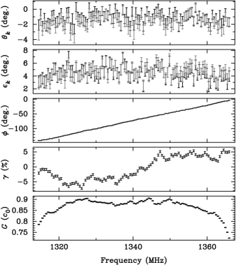
Figure 2: Best-fit instrumental parameters as a function of observing frequency. From top to bottom are plotted the orientations, $\theta_{k}$, and ellipticities, $\epsilon_{k}$, of the feed receptors, the differential phase, $\phi$, the differential gain ratio, $\gamma$, and the absolute gain, $G$. In the top two panels, black and gray correspond to receptors $\mbox{\boldmath$r$}_{0}$ and $\mbox{\boldmath$r$}_{1}$, respectively.

In each 500 kHz channel, it is possible to estimate the ellipticities and orientations of the feed receptors with an uncertainty of only $1\arcdeg$. The apparent correlation between these angles indicates that the non-orthogonality of the receptors, $\delta_{\theta}$ and $\delta_{\epsilon}$, is better constrained than their absolute positions. As a function of frequency, the differential gain ratio, $\gamma$, exhibits a peak-to-peak variation of about 10%. If not properly calibrated, these deviations will result in severe systematic distortion of arrival times derived from the total intensity profile (cf. Table 2). Furthermore, the effect on the frequency-integrated profile may vary randomly in time due to interstellar scintillation of the pulsar signal. Figure 2 emphasizes the importance of calibrating with sufficiently high frequency resolution to avoid bandwidth depolarization (van Straten, 2002), an irreversible effect that cannot be modeled in the current formulation of matrix template matching.

6 Conclusions

The future of high-precision pulsar timing is inextricably linked with advances in high-fidelity polarimetry. For one out of the six selected pulsars, the improvement in precision yielded by matrix template matching is better than that produced by doubling the integration length or instrumental bandwidth. In the analysis of the conventional method of scalar template matching, conservative levels of instrumental distortion are predicted to produce systematic timing errors of the same order as the rms timing residuals in the current best data sets. These errors are completely eliminated by the matrix template matching method. Therefore, it is expected this technique will perform better than current conventional methods in the majority of experiments. Furthermore, the method provides a new means of fully calibrating the instrumental response using a single observation of a well-determined pulsar.

Implicit in the application of the matrix template matching method is the assumption that the average polarization intrinsic to the pulsar does not vary significantly over any timescale of interest. Although a variety of studies have investigated the large fluctuations in the polarization of single pulses (e.g. Edwards (2004), Karastergiou & Johnston (2004), and references therein) no research on the long term properties of pulsar polarization has been published to date. Most likely, any process that effects phase-dependent changes in average polarization would similarly alter the total intensity profile. Therefore, a systematic study of the long term stability of millisecond pulsar polarization would make a valuable contribution toward the major science goals of this field, such as the detection of low-frequency gravitational radiation and the verification of relativistic gravity in the strong-field limit (Cordes et al., 2004; Hobbs, 2005, and references therein).

The impact of polarization on pulsar timing will become increasingly apparent in a larger number of experiments as instruments with greater sensitivity are employed, and it is imperative to incorporate a sophisticated treatment of polarization in high-precision timing analyses. All of the software required to perform matrix template matching is freely available as part of PSRCHIVE (Hotan, van Straten, & Manchester, 2004), which has been openly developed in an effort to facilitate the exchange of pulsar astronomical data between observatories and research groups.

The following additional material was not submitted to The Astrophysical Journal and was not peer reviewed. It is provided as further information for the interested reader.

Appendix A Equation (13): Conditional Variance of $\varphi$

Equation (13) presents an analytical expression for the conditional variance of the best-fit phase shift. Given only the template profile, it can be used to predict arrival time precision as a function of the $S/N$ of the observation. There are two ways to derive Equation (13):

1. via Equations (11) and (12); i.e. using the $\sin(x)=x$ small-angle approximation, solving for the slope, and applying first-order error propagation; or

2. via Equation (14), which defines the curvature matrix from which the uncertainty of the $\varphi$ estimate is formally defined.

Both derivations are shown here.

A.1 Derivation via Equations (11) and (12)

Start by deriving Equation (11), noting that Equation (10) can be written

$$\chi^{2}=\sum_{m=1}^{N/2}\sum_{k=0}^{3}\varsigma_{k}^{-2}\Delta_{k,m}\Delta^{*}_{k,m},$$ (A1)

where

$$\Delta_{k,m}=S_{k}^{\prime}(\nu_{m})-{\rm tr}[\mbox{\boldmath$\sigma$}_{k}\;\mbox{\boldmath$\rho$}^{\prime}(\nu_{m})],$$ (A2)

such that

$${\partial\chi^{2}\over\partial\varphi}=\sum_{m=1}^{N/2}\sum_{k=0}^{3}\varsigma_{k}^{-2}2{\rm Re}\left[\Delta^{*}_{k,m}{\partial\Delta_{k,m}\over\partial\varphi}\right].$$ (A3)

Now

$${\partial\Delta_{k,m}\over\partial\varphi}=i2\pi\nu_{m}{\rm tr}\left[\mbox{\boldmath$\sigma$}_{k}\;\mbox{\boldmath$\rho$}^{\prime}(\nu_{m})\right]$$ (A4)

and ${\rm Re}[iz]=-{\rm Im}[z]$; therefore,

$${\partial\chi^{2}\over\partial\varphi}=-4\pi\sum_{m=1}^{N/2}\sum_{k=0}^{3}\varsigma_{k}^{-2}\nu_{m}{\rm Im}\left[\Delta^{*}_{k,m}{\rm tr}\left[\mbox{\boldmath$\sigma$}_{k}\;\mbox{\boldmath$\rho$}^{\prime}(\nu_{m})\right]\right].$$ (A5)

In the above equation, the second term of $\Delta^{*}_{k,m}$ is multiplied by its complex conjugate, resulting in a real number (the squared modulus) with no imaginary component; therefore,

$${\partial\chi^{2}\over\partial\varphi}=-4\pi\sum_{m=1}^{N/2}\sum_{k=0}^{3}\varsigma_{k}^{-2}\nu_{m}{\rm Im}\left[S_{k}^{\prime*}(\nu_{m}){\rm tr}\left[\mbox{\boldmath$\sigma$}_{k}\;\mbox{\boldmath$\rho$}^{\prime}(\nu_{m})\right]\right].$$ (A6)

Now define the cross-spectral power of the template and the observation

$$S_{k,m}=S_{k}^{\prime*}(\nu_{m}){\rm tr}\left[\mbox{\boldmath$\sigma$}_{k}\;\mbox{\boldmath$\rho$}_{0}(\nu_{m})\right],$$ (A7)

such that

$${\partial\chi^{2}\over\partial\varphi}=-4\pi\sum_{m=1}^{N/2}\sum_{k=0}^{3}\varsigma_{k}^{-2}\nu_{m}{\rm Im}\left[S_{k,m}\exp(-i2\pi\nu_{m}\varphi)\right].$$ (A8)

Equation (11) is obtained after expressing $S_{k,m}$ in polar coordinates; Equation (12) is a small angle (or high $S/N$) approximation. Note that the opening minus sign is missing in these equations.

To derive Equation (13), first solve Equation (12) for $\varphi$

$$\varphi={\mbox{\boldmath$\sum$}\varsigma_{k}^{-2}|S_{k,m}|\phi_{k,m}\nu_{m}\over 2\pi\mbox{\boldmath$\sum$}\varsigma_{k}^{-2}|S_{k,m}|\nu_{m}^{2}},$$ (A9)

where $\mbox{\boldmath$\sum$}=\sum_{m=1}^{N/2}\sum_{k=0}^{3}$ is introduced for convenience. Standard error propagation is greatly simplified by recognizing that the variance of $\phi_{k,m}$ is $|S_{k,m}|$. Therefore, to first order, the variance of $\varphi$ is given by

$${\rm var}(\varphi)=\sum_{m=1}^{N/2}\sum_{k=0}^{3}\left({\partial\varphi\over\partial\phi_{k,m}}\right)^{2}\varsigma_{k}^{-2}|S_{k,m}|$$ (A10)

Substitution of

$${\partial\varphi\over\partial\phi_{k,m}}={\varsigma_{k}^{-2}|S_{k,m}|\nu_{m}\over 2\pi\mbox{\boldmath$\sum$}\varsigma_{k}^{-2}|S_{k,m}|\nu_{m}^{2}}$$ (A11)

into equation A10 yields

$${\rm var}(\varphi)=\sum_{m=1}^{N/2}\sum_{k=0}^{3}{\varsigma_{k}^{-2}|S_{k,m}|\nu_{m}^{2}\over 4\pi^{2}\left(\mbox{\boldmath$\sum$}\varsigma_{k}^{-2}|S_{k,m}|\nu_{m}^{2}\right)^{2}}={1\over 4\pi^{2}\mbox{\boldmath$\sum$}\varsigma_{k}^{-2}|S_{k,m}|\nu_{m}^{2}},$$ (A12)

which, after expanding $\sum$, yields Equation (13).

A.2 Derivation via Equation (14)

When no other parameters are varied, the conditional variance,

$${\rm var}(\varphi|{\bf J})=c_{\varphi\varphi}=\alpha_{00}^{-1}$$ (A13)

where $\alpha$ is the $1\times 1$ curvature matrix defined by Equation (14) and

$$\alpha_{00}={1\over 2}{\partial^{2}\chi^{2}\over\partial\varphi\partial\varphi}={2\over\varsigma^{2}}\sum_{m=1}^{N/2}{\rm Re}\left[{\rm tr}\left({\partial\mbox{\boldmath$\rho$}^{\prime\dagger}_{m}\over\partial\varphi}{\partial\mbox{\boldmath$\rho$}^{\prime}_{m}\over\partial\varphi}\right)\right].$$ (A14)

Using

$${\partial\mbox{\boldmath$\rho$}^{\prime}_{m}\over\partial\varphi}=-i2\pi\nu_{m}\mbox{\boldmath$\rho$}^{\prime}_{m}$$ (A15)

and

$${\rm tr}(\mbox{\boldmath$\rho$}^{\dagger}\mbox{\boldmath$\rho$})={1\over 2}\sum_{k=0}^{3}S_{k}S_{k}^{*},$$ (A16)

Equation (A14) becomes

$$\alpha_{00}={4\pi\over\varsigma^{2}}\sum_{m=1}^{N/2}\nu_{m}^{2}\sum_{k=0}^{3}|S_{k,m}|$$ (A17)

which, in turn, yields Equation (13) if it is assumed that $\varsigma_{k}=\varsigma$.

A.3 Interpretation

1. Equation (13) is the Fourier domain representation of Equation (B1) of Downs & Reichley (1983); this can be proven by noting that, if $X(\nu)$ is the Fourier transform of $x(\phi)$, then $i2\pi\nu X(\nu)$ is the Fourier transform of $dx/d\phi$ and, by Parseval’s Theorem, the integral of $[dx/d\phi]^{2}$ in the phase domain is equal to the integral of $\nu^{2}|X(\nu)|^{2}$ in the frequency domain.

2. Phases such as $\phi_{n}=n/N$ and $\varphi$ are dimensionless turns; therefore, TOA $\tau=\tau_{0}+\varphi P$, where $P$ is the pulse period.

3. Frequencies such as $\nu_{m}=m$ are dimensionless harmonics.

4. $S_{k,m}$ is the cross spectral power between the template and profile; in the case of the theoretical prediction, it is the autospectral power in the template.

5. The r.m.s. of the noise in the Fourier domain $\varsigma_{k}$ is a function of the $S/N$ of the observation.

6. Equation (13) returns variance in dimensionless phase, which can be translated into arrival time error with $\sigma_{\tau}=\sqrt{{\rm var}(\varphi)}P$.

7. Based on the approximation, $\sigma_{\tau}=w(S/N)^{-1}$, were $w$ is the width of the pulse, Equation (13) can be used to define the effective width of a pulse.

Appendix B Equation (14): Curvature Matrix

Begin with the definition of the merit function,

$$\chi^{2}=\sum_{m=1}^{N/2}\sum_{k=0}^{3}{|S_{k}^{\prime}(\nu_{m})-{\rm tr}[\mbox{\boldmath$\sigma$}_{k}\,\mbox{\boldmath$\rho$}^{\prime}(\nu_{m})]|^{2}\varsigma_{k}^{-2}}.$$ (B1)

Letting $\mbox{\boldmath$\rho$}^{\prime}_{m}=\mbox{\boldmath$\rho$}^{\prime}(\nu_{m})$ and $\varsigma_{k}=\varsigma$, the first partial derivative is

$${\partial\chi^{2}\over\partial\eta_{r}}=-{2\over\varsigma^{2}}\sum_{m=1}^{N/2}\sum_{k=0}^{3}{\rm Re}\left[(S_{k}^{\prime}(\nu_{m})-{\rm tr}[\mbox{\boldmath$\sigma$}_{k}\,\mbox{\boldmath$\rho$}^{\prime}_{m}]){\rm tr}\left(\mbox{\boldmath$\sigma$}_{k}\,{\partial\mbox{\boldmath$\rho$}^{\prime}_{m}\over\partial\eta_{r}}\right)^{*}\right]$$ (B2)

Because the Pauli spin matrices are Hermitian, ${\rm tr}(\mbox{\boldmath$\sigma$}_{k}\,\mbox{\boldmath$\rho$})^{*}={\rm tr}(\mbox{\boldmath$\sigma$}_{k}\,\mbox{\boldmath$\rho$}^{\dagger})$. The second partial derivative is

$${\partial^{2}\chi^{2}\over\partial\eta_{r}\partial\eta_{s}}={2\over\varsigma^{2}}\sum_{m=1}^{N/2}\sum_{k=0}^{3}{\rm Re}\left[{\rm tr}\left(\mbox{\boldmath$\sigma$}_{k}\,{\partial\mbox{\boldmath$\rho$}^{\prime}_{m}\over\partial\eta_{s}}\right){\rm tr}\left(\mbox{\boldmath$\sigma$}_{k}\,{\partial\mbox{\boldmath$\rho$}^{\prime\dagger}_{m}\over\partial\eta_{r}}\right)\right].$$ (B3)

Following the discussion in § 15.5 of Numerical Recipes, the term containing a second derivative in equation (14) has been dropped. Now the trace of a matrix is a scalar and $c\,{\rm tr}({\bf A})={\rm tr}(c{\bf A})$; therefore,

$${\partial^{2}\chi^{2}\over\partial\eta_{r}\partial\eta_{s}}={2\over\varsigma^{2}}\sum_{m=1}^{N/2}\sum_{k=0}^{3}{\rm Re}\left[{\rm tr}\left({\rm tr}\left[\mbox{\boldmath$\sigma$}_{k}\,{\partial\mbox{\boldmath$\rho$}^{\prime}_{m}\over\partial\eta_{s}}\right]\mbox{\boldmath$\sigma$}_{k}\,{\partial\mbox{\boldmath$\rho$}^{\prime\dagger}_{m}\over\partial\eta_{r}}\right)\right]$$ (B4)

Furthermore ${\rm tr}({\bf A})+{\rm tr}({\bf B})={\rm tr}({\bf A}+{\bf B})$ and ${\rm Re}(z)+{\rm Re}(w)={\rm Re}(z+w)$, so

$${\partial^{2}\chi^{2}\over\partial\eta_{r}\partial\eta_{s}}={2\over\varsigma^{2}}\sum_{m=1}^{N/2}{\rm Re}\left[{\rm tr}\left(\left[\sum_{k=0}^{3}{\rm tr}\left(\mbox{\boldmath$\sigma$}_{k}\,{\partial\mbox{\boldmath$\rho$}^{\prime}_{m}\over\partial\eta_{s}}\right)\mbox{\boldmath$\sigma$}_{k}\right]{\partial\mbox{\boldmath$\rho$}^{\prime\dagger}_{m}\over\partial\eta_{r}}\right)\right].$$ (B5)

The first factor inside the trace,

$$\sum_{k=0}^{3}{\rm tr}\left(\mbox{\boldmath$\sigma$}_{k}\,{\partial\mbox{\boldmath$\rho$}^{\prime}_{m}\over\partial\eta_{s}}\right)\mbox{\boldmath$\sigma$}_{k}=2{\partial\mbox{\boldmath$\rho$}^{\prime}_{m}\over\partial\eta_{s}}$$ (B6)

and ${\rm tr}({\bf AB})={\rm tr}({\bf BA})$; therefore

$${\partial^{2}\chi^{2}\over\partial\eta_{r}\partial\eta_{s}}={4\over\varsigma^{2}}\sum_{m=1}^{N/2}{\rm Re}\left[{\rm tr}\left({\partial\mbox{\boldmath$\rho$}^{\prime\dagger}_{m}\over\partial\eta_{r}}{\partial\mbox{\boldmath$\rho$}^{\prime}_{m}\over\partial\eta_{s}}\right)\right].$$ (B7)

Appendix C Equation (28): Non-orthogonality, $\sin(\delta)$

Begin with

$$\cos 2\delta=-\cos\Theta=-{\mbox{\boldmath$S$}_{0}\mbox{\boldmath$\cdot$}\mbox{\boldmath$S$}_{1}\over|\mbox{\boldmath$S$}_{0}||\mbox{\boldmath$S$}_{1}|}=1-2\left({|\mbox{\boldmath$r$}_{0}^{\dagger}\mbox{\boldmath$r$}_{1}|\over|\mbox{\boldmath$r$}_{0}||\mbox{\boldmath$r$}_{1}|}\right)^{2}$$ (C1)

then use the double-angle formula $\cos 2\delta=1-2\sin^{2}\delta$.

References

- Born & Wolf (1980) Born, M., & Wolf, E. 1980, Principles of Optics (Cambridge: Cambridge Univ. Press)
- Britton (2000) Britton, M. C. 2000, ApJ, 532, 1240
- Britton et al. (2000) Britton, M. C., van Straten, W., Bailes, M., Toscano, M., & Manchester, R. N. 2000, in IAU Colloq. 177, Pulsar Astronomy - 2000 and Beyond, ed. M. Kramer, N. Wex, & R. Wielebinski (San Francisco: ASP), 73
- Chandrasekhar (1960) Chandrasekhar, S. 1960, Radiative Transfer (New York: Dover)
- Cordes et al. (2004) Cordes, J. M., Kramer, M., Lazio, T. J. W., Stappers, B. W., Backer, D. C., & Johnston, S. 2004, New Astr. Rev., 48, 1413
- Downs & Reichley (1983) Downs, G. S., & Reichley, P. E. 1983, ApJS, 53, 169
- Edwards (2004) Edwards, R. T. 2004, A&A, 426, 677
- Hamaker (2000) Hamaker, J. P. 2000, A&AS, 143, 515
- Hobbs (2005) Hobbs, G. 2005, Proc. Astr. Soc. Aust., 22, 179
- Hotan, Bailes, & Ord (2004) Hotan, A. W., Bailes, M., & Ord, S. M. 2004, MNRAS, 355, 941
- Hotan, van Straten, & Manchester (2004) Hotan, A. W., van Straten, W., & Manchester, R. N. 2004, Proc. Astr. Soc. Aust., 21, 302
- Jacoby et al. (2005) Jacoby, B. A., Hotan, A., Bailes, M., Ord, S., & Kulkarni, S. R. 2005, ApJ, 629, L113
- Jenet et al. (2005) Jenet, F. A., Hobbs, G. B., Lee, K. J., & Manchester, R. N. 2005, ApJ, 625, L123
- Karastergiou & Johnston (2004) Karastergiou, A. & Johnston, S. 2004, MNRAS, 352, 689
- Lommen & Backer (2001) Lommen, A. N. & Backer, D. C. 2001, ApJ, 562, 297
- Ord et al. (2004) Ord, S. M., van Straten, W., Hotan, A. W., & Bailes, M. 2004, MNRAS, 352, 804
- Press et al. (1992) Press, W. H., Teukolsky, S. A., Vetterling, W. T., & Flannery, B. P. 1992, Numerical Recipes: The Art of Scientific Computing (2nd ed.; Cambridge: Cambridge Univ. Press)
- Splaver et al. (2005) Splaver, E. M., Nice, D. J., Stairs, I. H., Lommen, A. N., & Backer, D. C. 2005, ApJ, 620, 405
- Stairs (2004) Stairs, I. H. 2004, Science, 304, 547
- Stairs, Thorsett, & Camilo (1999) Stairs, I. H., Thorsett, S. E., & Camilo, F. 1999, ApJS, 123, 627
- Stuart, Ord, & Arnold (1999) Stuart, A., Ord, K., & Arnold, S. 1999, Kendall’s Advanced Theory of Statistics, Vol. 2A (6th ed.; New York: Oxford Univ. Press)
- Taylor (1992) Taylor, J. H. 1992, Philos. Trans. Roy. Soc. London A, 341, 117
- van Straten (2002) van Straten, W. 2004, ApJ, 568, 436
- van Straten (2003) van Straten, W. 2003, PhD thesis, Swinburne Univ. of Technology
- van Straten (2004) van Straten, W. 2004, ApJS, 152, 129
- van Straten (2005) van Straten, W. 2005, in ASP Conf. Ser. 328, Binary Radio Pulsars, ed. F. A. Rasio & I. H. Stairs, Vol. 328 (San Francisco: ASP), 383
- van Straten et al. (2001) van Straten, W., Bailes, M., Britton, M., Kulkarni, S. R., Anderson, S. B., Manchester, R. N., & Sarkissian, J. 2001, Nature, 412, 158