Density Profiles of Collisionless Equilibria. I. Spherical Isotropic Systems

Abstract

We investigate the connection between collisionless equilibria and the phase-space relation between density $\rho$ and velocity dispersion $\sigma$ found in simulations of dark matter halo formation, $F=\rho/\sigma^{3}\propto r^{-\alpha}$. Understanding this relation will shed light on the physics relevant to collisionless collapse and on the subsequent structures formed. We show that empirical density profiles that provide good fits to N-body halos also happen to have nearly scale-free $\rho/\sigma^{3}$ distributions when in equilibrium. We have also done a preliminary investigation of variables other than $r$ that may match or supercede the correlation with $F$. In the same vein, we show that $\rho/\sigma^{m}$, where $m=3$ is the most appropriate combination to use in discussions of the power-law relationship. Since the mechanical equilibrium condition that characterizes the final systems does not by itself lead to power-law $F$ distributions, our findings prompt us to posit that dynamical collapse processes (such as violent relaxation) are responsible for the radial power-law nature of the $\rho/\sigma^{3}$ distributions of virialized systems.

1 Introduction

The “poor man’s” phase-space density proxy $F=\rho/\sigma^{3}$, where $\rho$ is density and $\sigma$ is total velocity dispersion, is a power-law in radius ($F\propto r^{-\alpha}$) for a surprising variety of self-gravitating, collisionless equilibria. Isothermal systems have $\rho\propto r^{-2}$ and constant $\sigma$, giving $\alpha=2$. A broader class of systems with power-law behavior in both $\rho$ and $\sigma$ also naturally produce power-law behavior for $F$. For example, the self-similar collisionless infall models in Bertschinger (1985, §4) have $\rho\propto r^{-9/4}$ and $\sigma\propto r^{-1/8}$, leading to $\alpha=1.875$. More surprising is that systems in which neither $\rho$ nor $\sigma$ are power-laws can still possess $F$ distributions that are. For example, there is a growing body of evidence, supported by results from simulations of increasingly higher resolution and detail, that seems to suggest collisionless halos formed in cosmological simulations are characterized by nearly scale-free $F$ distributions, although they have decidedly nonpower-law density profiles. This was first noted by Taylor & Navarro (2001) who, at the time, determined that $\alpha=1.875$ over 3 orders of magnitude in radius. This value of $\alpha$, coincidently, is the same as that derived by Bertschinger (1985). More recent N-body simulations have produced $\alpha$ values of; 1.95 (Raisa et al., 2004), 1.90 (Ascasibar et al., 2004), and 1.84 (Dehnen & McLaughlin, 2005, based on the simulations in Diemand, Moore, & Stadel (2004a, b)). Austin et al. (2005) report that a very different, semi-analytical halo formation method results in power-law $F$ distributions over similar radial ranges. However, these authors find a range of $\alpha$ values (including 1.875) that depend on initial conditions. As this formation method is much simpler than an N-body evolution but still reproduces scale-free $F$, the physics responsible for the distribution must be common to both techniques. One such process is violent relaxation. In this work, we use “violent relaxation” as shorthand for the incomplete relaxation process that is due to the varying of potential during collapse rather than the strict, complete relaxation discussed in Lynden-Bell (1967). Also in the Austin et al. (2005) work, it is shown that in a totally isotropic system the Jeans equation can be solved analytically and that there is a “special” $\alpha=35/18=1.94\bar{4}$.

It appears that power-law distributions of $F$ are robust features of collisionless equilibria. The exponents of the power-laws vary, but cluster near values $\lesssim 2$. This paper is part of a continuing series of investigations aimed at understanding the ubiquity and the origin of the phenomenon. We specifically want to exploit its occurence to gain insights into the processes governing the virialization of collisionless halos.

In this paper, we review the conditions for hydrostatic equilibrium, the Jeans equation. By examining density profiles motivated by N-body simulations and analyzing the associated $F$ distributions, in §3 we demonstrate that the Jeans equation by itself is not sufficient to force a power-law for $\rho/\sigma^{3}$. At present, we restrict ourselves to spherical equilibria with isotropic velocity distributions. Interestingly, typical density profiles that are used to characterize data from cosmological N-body simulations all seem to have nearly scale-free $F$ distributions, as do halos that are formed semi-analytically (Austin et al., 2005). This aspect of N-body and semi-analytically generated halos is certainly unexpected and consequently, in §4, we investigate the implications of explicitly imposing the requirement of scale-free $\rho/\sigma^{3}$ on the density profiles of equilibrium structures. We summarize our findings in the final section.

2 Empirical Density Profiles

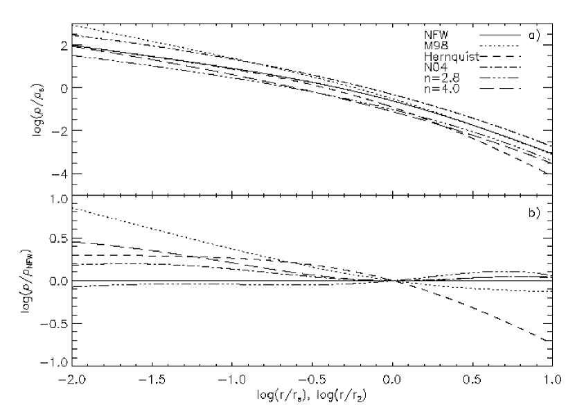
Figure 1: Plots showing the NFW (solid line), Moore et al. (1998) (dotted), Hernquist (dashed), Navarro et al. (2004) (dash-dotted), Sérsic $n=2.8$ (dash-triple dotted), and Sérsic $n=4.0$ (long dashed) density distributions. The linestyles are the same in both plots. a) The log-log density profiles. The vertical normalization is arbitrary and the curves have been somewhat separated to aid identification. b) The log-log density profiles of the same distributions divided the NFW (horizontal solid line). These ratio profiles have been normalized to agree at the scale radius.

In this work we will focus on several specific density profiles, shown in Figures 1 & 2. The standard Navarro-Frenk-White (Navarro et al., 1996, 1997, NFW), Moore et al Moore et al. (1998, M98), and Hernquist (Hernquist, 1990) (solid, dotted, and dashed lines, respectively) are examples of dual power-law distributions with differing asymptotic behaviors that have been used to fit density profiles of cosmological N-body halos. The generalized dual power-law profile has the form,

$$\frac{\rho}{\rho_{s}}=\left(\frac{r}{r_{s}}\right)^{-c_{1}}\left(1+\frac{r}{r_{s}}\right)^{-c_{2}},$$ (1)

where $\rho_{s}$ and $r_{s}$ are a scale density and length, respectively. The exponents $c_{1}$ and $c_{2}$ determine the asymptotic power-law behavior of the profile; NFW: ($c_{1}=1,\ c_{2}=2$), M98: ($c_{1}=1.5=c_{2}$), Hernquist: ($c_{1}=1,\ c_{2}=3$). We define the negative logarithmic density slope to be $\gamma\equiv-d\log{(\rho/\rho_{s})}/d\log{(r/r_{s})}$. For generalized dual power-law profiles, the $\gamma$ distributions are given by,

$$\gamma=\frac{c_{1}+(c_{1}+c_{2})(r/r_{s})}{1+(r/r_{s})}.$$ (2)

The Navarro et al. (2004) profile (dash-dotted line) has been proposed as an improvement over NFW for describing high resolution cosmological N-body density profiles. This profile never displays power-law behavior; instead, the logarithmic density slope changes continuously with $r$. The expression that generates this curve is,

$$\ln{\left(\frac{\rho}{\rho_{2}}\right)}=-\left(\frac{2}{\mu}\right)\left[\left(\frac{r}{r_{2}}\right)^{\mu}-1\right],$$ (3)

where $r_{2}$ is the radius where $\gamma=2$ and $\rho_{2}$ is the density at that radius. The corresponding $\gamma$ profile is,

$$\gamma=2\left(\frac{r}{r_{2}}\right)^{\mu}.$$ (4)

As Navarro et al. (2004) found that $\mu=0.17$ best fit several N-body halo profiles, we will refer to profiles ($\rho$ and $\gamma$) with $\mu=0.17$ as N04 profiles, but we consider $0.001\leq\mu\leq 0.22$.

The final profile type we consider is the Sérsic function (Sérsic, 1968). The Sérsic function is expressed analytically as,

$$\ln{\left(\frac{\Sigma}{\Sigma_{s}}\right)}=-a_{n}\left[\left(\frac{R}{R_{s}}\right)^{1/n}-1\right],$$ (5)

where $\Sigma$ is surface density, $R$ is projected distance, $n$ determines the shape of the profile, and $a_{n}$ is an $n$ dependent constant chosen so that the projected mass interior to $R_{s}$ is equal to the projected mass interior to $R=r_{2}$ for the N04 profile, Equation 3. This differs from the usual definition of the Sérsic constant that demands the projected mass within $R_{s}$ be half the total mass. Unfortunately, Sérsic profiles do not readily provide analytical expressions for $\rho$ or $\gamma$ [but see Trujillo et al. (2002) and Graham et al. (2005)]. The dash-triple dotted and long dashed lines in Figure 1 show the calculated deprojected density distributions for $n=2.9$ and $n=4.0$ (de Vaucouleurs profile), respectively. Larger (smaller) $n$ values reduce (increase) the difference between the inner and outer logarithmic density slopes. Dalcanton & Hogan (2001) and Merritt et al. (2005) both suggest that the Sérsic profile describes the results of N-body simulations at least as well as the previously discussed forms. Further, Dalcanton & Hogan (2001) point out that $n\lesssim 4$ Sérsic and NFW profiles have similar behaviors while Merritt et al. (2005) find that $n\approx 3$ provides the best fit to their dwarf and galaxy-sized halos.

3 $\rho/\sigma^{3}$ Distributions & Equilibrium

Mechanical equilibrium for a spherical and isotropic collisionless system is determined through the Jeans equation (Jeans, 1919; Binney & Tremaine, 1987),

$$\frac{d}{dr}\left[\rho(r)\sigma^{2}(r)\right]=-3G\rho(r)\frac{M(r)}{r^{2}},$$ (6)

where $M(r)$ is the mass enclosed at radius $r$ and the factor of 3 comes from the definition $\sigma^{2}=\sigma_{r}^{2}+\sigma_{\theta}^{2}+\sigma_{\phi}^{2}$ and the isotropy of the system. This equation certainly links $\rho$ and $\sigma$, but does it alone impose power-law $F$ distributions?

3.1 Specific Distributions

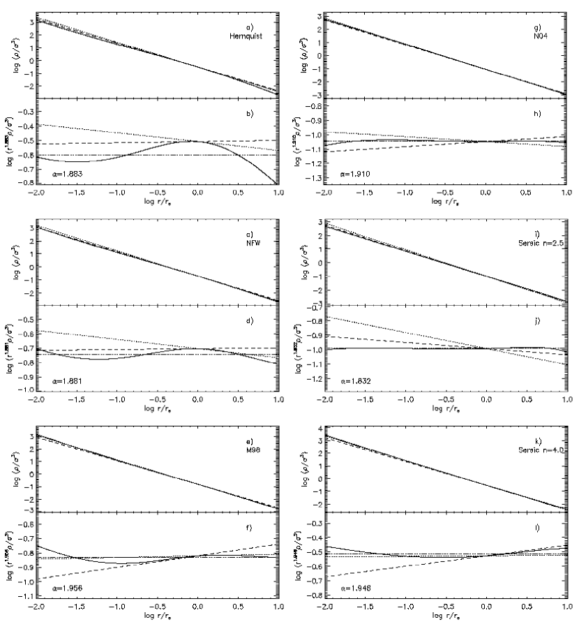
Figure 2: Plots showing the raw $F$ distributions (panels a, c, e, g, i, k) and versions scaled to highlight departures from a pure power-law (panels b, d, f, h, j, l). The dashed and dotted lines show the behavior of power-law $F$ distributions with $\alpha=1.875$ and $\alpha=35/18$, respectively. The $\alpha$ values indicated in the bottom panels are the slopes of the lines that best-fit the scaled profiles. Also in the bottom panels, the scaled best linear fits are the dash-triple dotted horizontal lines, and the dotted and dashed lines are the scaled power-laws corresponding to the lines in the upper panels. The density profiles are noted in the plots; Hernquist (a,b), NFW (c,d), Moore et al. (1998) (e,f), Navarro et al. (2004) (g,h), Sérsic $n=2.5$ (i,j), and Sérsic $n=4.0$ (k,l).

We demonstrate that the answer is no by providing a counter-example. Inserting the Hernquist density profile into Equation 6, we solve for $\sigma$ and thereby insure that the halo is in equilibrium. The resulting $F$ distribution is shown as a solid line in Figure 2, panels a and b. In the top panels of this figure, the dashed lines have slopes of -1.875, the dotted lines have slopes of -35/18, and each line is normalized to the $F$ value at $\log{(r/r_{s})}=0$. The curves in the bottom panels highlight departures from the best-fit power-law behavior (horizontal dash-triple dotted lines). The dashed and dotted lines denote the same power-laws as in the top panels, but scaled to the best-fit slope. We use $\alpha=1.875$ as a fiducial value because it is the result of straightforward analytical calculation (Bertschinger, 1985) as well as being representative of the mean of the N-body results discussed in the Introduction. At the same time, we will also highlight the analytically motivated $\alpha=35/18$ (Austin et al., 2005). The abscissa range for the figure reflects that halos are usually resolved over roughly 3 orders of magnitude, from the virial radius [$\log{(r/r_{s})}\approx 1$] to about 1/1000 of the virial radius [$\log{(r/r_{s})}\approx-2$]. The dash-triple dotted lines in the bottom panels indicate the best linear fits to the $F$ profiles. The dotted and dashed lines represent the same lines as in the top panel rescaled to the best linear fit slope. The $\alpha$ values indicate the slope (modulo a minus sign) that the best linear fit would have in the top panel.

We use the rms deviations $\Delta_{\rm rms}$ between the $F$ distributions and the best power-law fits to quantify how close to a power-law each $F$ is. These deviations are calculated over the resolved range of N-body halos, from $\log{(r/r_{s})}\approx-2$ to $\log{(r/r_{s})}\approx 1$. We adopt the following convention for the rest of the paper; $F$ distributions with $\Delta_{\rm rms}\leq 0.05$ will be considered power-laws, those with $\Delta_{\rm rms}>0.05$ will not. This approximately reflects the level at which one can detect a power-law by eye, e.g., by looking at panel a. With this criterion, the Hernquist profile, with $\Delta_{\rm rms}=0.07$, is evidence that simple mechanical equilibrium does not enforce power-law $F$ behavior. The Hernquist profile is not unique in this regard; King models (King, 1966, not discussed in detail here) also produce $F$ distributions that have quite obvious deviations from power-law shapes.

Having found these counter-examples, we now demonstrate that the other empirical density profiles from §2 generally lead to scale-free $F$ distributions. In Figure 2, we present the $F$ distributions calculated by solving Equation 6 using the NFW (panels c and d), M98 (e and f), and N04 (g and h) density profiles. These profiles have power-law $F$ distributions with $\Delta_{\rm rms}\lesssim 0.03$ and $\alpha=1.881$, 1.956, and 1.910 for NFW, M98, and N04, respectively. N04 produces the best power-law $F$ distribution of these 3 models, with $\Delta_{\rm rms}=0.007$. NFW and M98 profiles are poorer (but still acceptable) power-laws with $\Delta_{\rm rms}\approx 0.03$. Sérsic profiles also produce power-law $F$ distributions, with the best power-law $F$ ($n=2.5$, $\Delta_{\rm rms}=0.005$, $\alpha=1.832$) shown in Figure 2 panels i and j. We also include the results from the de Vaucouleurs profile (Sérsic $n=4.0$) in panels k and l. This range of $\alpha$ values (1.83-1.96) is approximately the same as the range of results from N-body simulations (see the Introduction). These findings are also in broad agreement with the results of Graham et al. (2005).

3.2 General Distributions

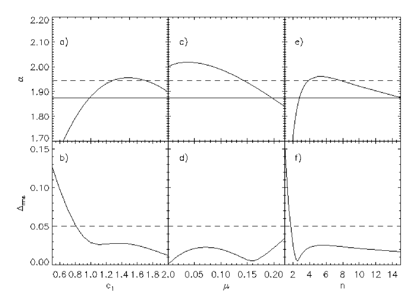
Figure 3: Plot of the $\alpha$ and $\Delta_{\rm rms}$ values versus the shape parameters for generalized dual power-law profiles (panels a & b), N04 profiles (panels c & d), and Sérsic profiles (panels e & f). The shape parameters are $c_{1}$ ($c_{2}=3-c_{1}$), $\mu$, and $n$ for the dual-power law, N04, and Sérsic profiles, respectively. In the top panels, the solid line lies at $\alpha=1.875$ and the dashed line marks $\alpha=35/18$. The dashed line in the bottom panels illustrates the acceptable power-law cut-off value of $\Delta_{\rm rms}=0.05$.

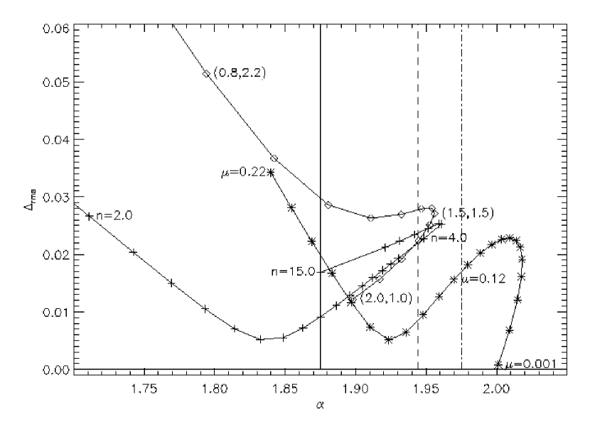
Figure 4: $\alpha$ versus $\Delta_{\rm rms}$ for generalized dual power-law (diamonds), N04 (asterisks), and Sérsic (plus symbols) profiles. Along the Sérsic track, the $n$ values increase from 2 to 15, with a turnaround point at $n=5$. The $\mu$ values decrease from left to right ($0.22\rightarrow 0.001$) along the N04 track. The upper-leftmost diamond has ($c_{1}=0.8,c_{2}=2.2$), the diamond with the largest $\alpha$ corresponds to the M98 profile ($c_{1}=c_{2}=1.5$), and the diamond with the smallest $\Delta_{\rm rms}$ has ($c_{1}=2.0,c_{2}=1.0$). The NFW ($c_{1}=1.0,c_{2}=2.0$) profile is marked by the diamond nearest to the solid line at $\alpha=1.875$. The dashed and dash-dotted lines mark $\alpha=35/18$ and $\alpha=1.975$, respectively.

In addition to these specific profiles, we have also examined the generic forms of Equations 1, 3, and 5. Varying the shape parameters ($c_{1},c_{2},\mu,n$) of these profiles allows us to 1) find the profiles that have the best power-law $F$ behavior and 2) determine the ranges of $\alpha$ values that each profile supports. We summarize the findings in Figures 3 and 4.

Three classes of profiles are presented separately in Figure 3 to show the impact of the shape parameters on the $F$ distributions. Panels a and b display the results for generalized dual power-law profiles with the constraint that $c_{1}+c_{2}=3$ (like NFW and M98) and $0.5\leq c_{1}\leq 2.0$. One can see that $\alpha=1.875$ is obtained when $c_{1}\approx 1.0$ ($c_{2}\approx 2.0$), very nearly the canonical NFW profile. However, the shallow local minimum in panel b around $c_{1}=1.1$ indicates that the NFW profile does not give the best power-law $F$ (for isotropic systems). The shallowness of this minimum suggests that all values $1.0\lesssim c_{1}\lesssim 1.5$ give similar quality power-law $\rho/\sigma^{3}$ distributions. We note that the M98 profile ($c_{1}=1.5$) produces an $\alpha$ value closer to the analytical value of 35/18, with the ($c_{1}=1.3$) case providing the best fit to $\alpha=35/18$. We have also investigated a few profiles with $c_{1}+c_{2}=4$ and found that they do not form acceptable power-law $F$ distributions. Like the Hernquist profile ($c_{1}=1,c_{2}=3$), the $\Delta_{\rm rms}$ values for these profiles are always $>0.05$. The Navarro et al. (2004) profiles with $0.001\leq\mu\leq 0.22$ give rise to panels c and d. The $F$ distribution that produces the best power-law has $\mu\approx 0.16$, which is very close to the best-fit value $\mu=0.17$ from Navarro et al. (2004). For $\mu\approx 0.14$, the corresponding $\alpha\approx 35/18$. This range in $\mu$ values is consistent with halos found in the simulations of Navarro et al. (2004) $0.1\lesssim\mu\lesssim 0.2$. Among Sérsic profiles with $2.0\leq n\leq 15.0$ (panels e and f), the model at which $\Delta_{\rm rms}$ is minimum has $n=2.5$. This $n$ value lies in the range of values found in the Merritt et al. (2005) study. Interestingly, the Sérsic profile that produces $\alpha=35/18$ has $n\lesssim 4$, basically a deVaucouleurs profile.

Pursuing this further, we turn to Figure 4 which combines the results from the three profile types by relating $\alpha$ and $\Delta_{\rm rms}$ values. The plus symbols represent Sérsic profile values, asterisks mark Navarro et al. (2004) values, and diamonds show generalized dual power-law values. The vertical structure of this plot illustrates that the Navarro et al. (2004) and Sérsic profiles generally result in better power-law $F$ distributions than the dual power-law form. Interestingly, if we think of the various simulation-inspired profiles in chronological order (NFW, M98, and N04), it appears that the $\rho/\sigma^{3}$ distributions are becoming better power-laws as the number of particles in simulations increases, and the simulations themselves improve. Such a trend may be due to a decreased impact by two-body relaxation (which masks the dynamics relevant to actual halos and decreases in importance with increasing particle numbers) or it may be that the larger particle numbers allow simulations to more faithfully reflect the pertinent physics, e.g., violent relaxation.

In the horizontal direction of Figure 4, we clearly see that the profile types produce their best power-law at varying $\alpha$ values. However, the minimum value of $\Delta_{\rm rms}$ for all the profiles occur in a relatively narrow range of $\alpha$ values; between 1.84 and 1.97, close to the analytically derived value of $\alpha=1.94\bar{4}$. One thing to keep in mind is that this study deals only with isotropic systems. It could be that simulated N-body halos, which have anisotropic velocity distributions (Hansen & Moore, 2004; Barnes et al., 2005), are sufficiently different from these isotropic models to cause the offsets.

3.3 A More Fundamental Relation?

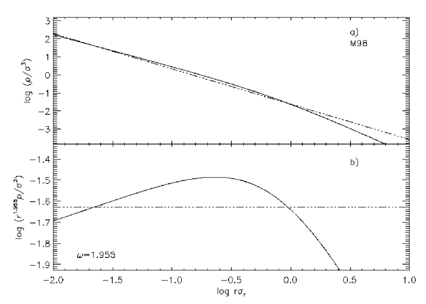
Figure 5: Representative curves showing the relationship between $\rho/\sigma^{3}$ and the radial action proxy $r\sigma_{r}$. These specific curves are for the M98 profile and should be compared to those in Figure 2 panels e and f. Panel a shows the raw correlation between $\log{F}$ and $\log{r\sigma_{r}}$ along with the best linear fit (dash-triple dotted line). Panel b displays the residuals between the best-linear fit and the actual correlation. The slope of the best-fit line is given by the $\omega$ value.

The scale-free realtionship between $F$ and $r$ has been firmly established, but we would like to know if there is a more dynamically relevant quantity that shows a similar power-law correlation with $F$. The list of candidate quantities is long, but we focus on two choices; enclosed mass $M(r)$ and a proxy for the radial action $r\sigma_{r}$. The $\log{F}$ vs. $\log{M}$ plots do not have power-law forms for any of the distributions. On the other hand, the $\log{F}$ vs.$\log{r\sigma_{r}}$ curves do have approximately scale-free shapes, as shown in Figure 5a. The best-fit line to this curve has a slope ($\omega=1.955$) that is very close the slope in Figure 2e ($\alpha=1.956$). However, the comparison between the residuals shown in Figure 5b and those in Figure 2f demonstrate that $F$ vs. $r$ is the better scale-free relation. Indeed, the near power-law relation between $F$ and $r\sigma_{r}$ occurs because $\sigma_{r}$ has a very weak relation on $r$, making $F$ vs. $r\sigma_{r}$ very similar to $F$ vs. $r$.

Hoeft, Mücket, & Gottlöber (2004) find that a nontrivial function of potential accurately describes the velocity dispersion profile in N-body halos. Utilizing a more general form of this function of potential,

$$A=\Phi^{a}(\Phi_{\rm out}-\Phi)^{b},$$ (7)

we have investigated whether or not $F$ vs. $A$ provides a superior power-law relation to $F$ vs. $r$. We find that with appropriate choices of $a$, $b$, and $\Phi_{\rm out}$, a power-law can be found for $F$ vs. $A$ that is of comparable quality to that for $F$ vs. $r$. However, we find that the degrees of freedom present in this function allow it to closely resemble $r$ itself, making this function unenlightening. Despite the results of this brief search for a more physically fundamental relation, we plan to continue investigating alternative dynamical quantities.

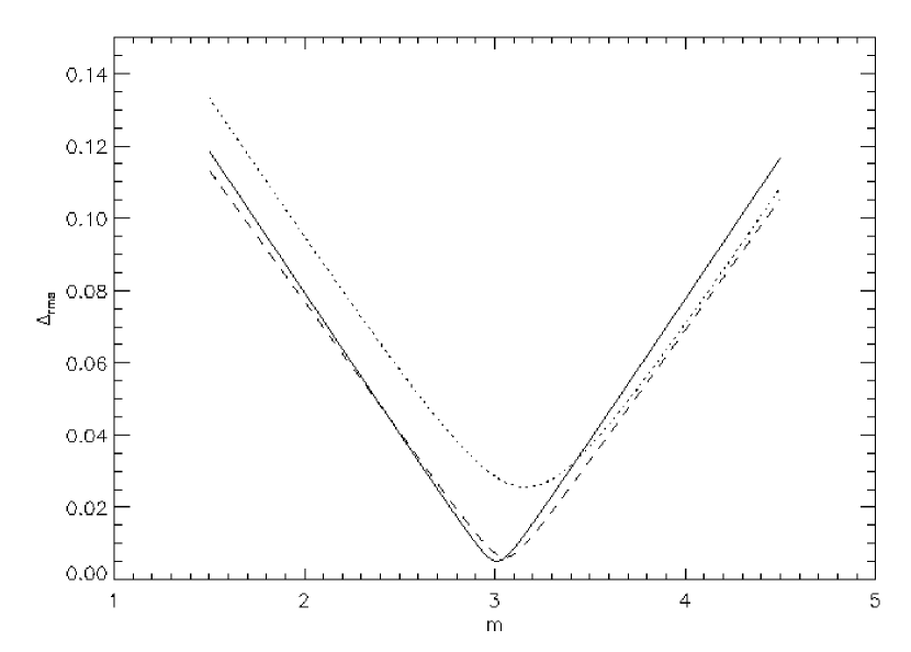
Figure 6: Curves showing that the best $\rho/\sigma^{m}$ vs. $r$ power-law occurs when $m=3$. The dotted line is the result of varying $m$ for an NFW profile, while the dashed and solid lines illustrate the variations for N04 and Sérsic $n=2.5$ profiles, respectively.

One could also question whether or not our $F$ function is the most illuminating choice of combination of $\rho$ and $\sigma$. Certainly, $\rho/\sigma^{3}$ is an interesting quantity, as it has the dimensions of phase-space density, but would $\rho/\sigma^{m}$ work just as well (R. Henriksen,, private comm., )? For the NFW, N04, and Sérsic functions, the answer is no. The deviations from a power-law distribution rapidly increase as $m$ varies from 3 (over the interesting radial range $-2\leq\log{r/r_{s}}\leq 1$). This affinity for $m=3$ is obvious in Figure 6 which shows the amplitude of the residuals from a power-law $F$ vs. $r$ relationship as $m$ is varied from 1.5 to 4.5.

In this section we have shown that the condition of hydrostatic equilibrium by itself does not produce power-law $\rho/\sigma^{3}$. However, the density profiles that are used to fit the data from cosmological N-body simulations all seem to have nearly scale-free $\rho/\sigma^{3}$ distributions, unlike the Hernquist and King profiles. We have also tried, in vain, to find more physically meaningful correlations between $F$ and other quantities; enclosed mass, $r\sigma_{r}$, etc. Furthermore, halos formed semi-analytically, through violent relaxation (Lynden-Bell, 1967), also display $F\propto r^{-\alpha}$ (Austin et al., 2005). This aspect of N-body and semi-analytically generated halos is certainly unexpected and prompts us to consider systems that have explicitly scale-free $\rho/\sigma^{3}$.

4 The Constrained Jeans Equation

Imposing the constraint that $\rho/\sigma^{3}=(\rho_{0}/v_{0}^{3})(r/r_{0})^{-\alpha}$ and using the dimensionless variables $x\equiv r/r_{0}$ and $y\equiv\rho/\rho_{0}$, we rewrite Equation 6 as,

$$-\frac{x^{2}}{y}\left[\frac{d}{dx}\left(y^{5/3}x^{2\alpha/3}\right)\right]=BM(x),$$ (8)

where $B=3G/r_{0}v_{0}^{2}$. Differentiating this equation with respect to $x$ gives us,

$$\frac{d}{dx}\left[-\frac{x^{2}}{y}\left\{\frac{d}{dx}\left(y^{5/3}x^{2\alpha/3}\right)\right\}\right]=Cyx^{2},$$ (9)

where $C=12\pi\rho_{0}r_{0}^{2}/v_{0}^{2}$. This expression is equivalent to that presented in Taylor & Navarro (2001). Following Austin et al. (2005), we eliminate the constant $C$ by solving for $y$, differentiating with respect to $x$ again, and grouping like terms. The resulting constrained Jeans equation is,

$$(2\alpha+\gamma-6)(\frac{2}{3}(\alpha-\gamma)+1)(2\alpha-5\gamma)=15\gamma^{\prime\prime}+3\gamma^{\prime}(8\alpha-5\gamma-5).$$ (10)

In this notation, $\gamma=\gamma(x)=-d\ln{y}/d\ln{x}$ and the primes indicate derivatives with respect to $\ln{x}$.

One way to connect power-law $F$ distributions and equilibria is by making an analogy to fluid systems. In hydrostatic equilibrium, the term on the left-hand side of Equation 6 is replaced by a derivative of a single variable, the pressure $P$ (related to the random motion in the system). The important point is that $P$ is related to $\rho$ through an equation of state. This extra relation closes the system of equations and, given boundary conditions, allows one to solve for the equilibrium density distribution. A power-law $F$ distribution acts as a radius-dependent equation of state, linking $\rho$ and the system’s random motion, measured by $\sigma$.

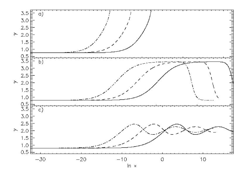
Figure 7: Various $\gamma$ distributions that result from solving Equation 10. The top panel shows solutions with $\alpha=1.875$. Panel b utilizes $\alpha=35/18$, and the bottom panel has $\alpha=1.975$. The solid lines in each panel are solutions with $\gamma^{\prime}=5\times 10^{-6}$. The dashed and dash-dotted lines have $\gamma^{\prime}=1\times 10^{-5}$ and $\gamma^{\prime}=5\times 10^{-5}$, respectively. The separations of the various profiles have been exaggerated for clarity.

Austin et al. (2005) demonstrate that this equation has a rich set of solutions that depend on the choices made for $\alpha$, initial $\gamma$ [$\gamma(0)$], and initial $\gamma^{\prime}$ [$\gamma^{\prime}(0)$]. In specific density profiles, the asymptotic behavior of $\gamma(x)$ can be made to increase without bound, to approach constant values, or even to oscillate. We show several types of solutions in Figure 7. We choose $\gamma(0)$ through the relation $2\alpha-5\gamma(0)=0$, representing a zero “pressure” derivative at the center (Austin et al., 2005). Once we choose an $\alpha$ value, the central $\gamma$ is set. This figure shows the impact of changing $\gamma^{\prime}(0)$ from $5\times 10^{-6}$ to $5\times 10^{-5}$ [see Austin et al. (2005) for examples of solutions with larger $\gamma^{\prime}(0)$ values]. Smaller values of $\gamma^{\prime}(0)$ force the $\gamma(x)$ distribution to change less rapidly with increasing $x$. Since changing $\gamma^{\prime}(0)$ values simply shifts $\gamma$ distributions horizontally and does not affect the overall shape (for $\gamma^{\prime}(0)\lesssim 10^{-3}$), we fix the $\gamma^{\prime}(0)$ value from here on. Larger $\gamma^{\prime}(0)$ values can make the $\gamma$ distribution convex in the region where $r=r_{s}$, unlike the distributions that are of interest here. Once $\gamma$ changes from its initial value, the behavior is largely determined by $\alpha$. As mentioned earlier, $\gamma$ profiles display one of three kinds of behavior and we choose to focus on three $\alpha$ values to provide concrete examples; $\alpha=1.875$, $\alpha=35/18$ , and $\alpha=1.975$. $\alpha=35/18$ divides solutions in which $\gamma(x)$ increases indefinitely (like those in the top panel with $\alpha=1.875$) from those in which $\gamma(x)$ acts as a damped oscillator (bottom panel with $\alpha=1.975$). A more extensive discussion of this special $\alpha$ value can be found in Austin et al. (2005, §3).

In previous sections, we have discussed many types of density profiles and have just shown that the constrained isotropic Jeans equation has a wide variety of solutions. We are now faced with the following questions; which (if any) of the density profiles from §3 provides the best description of the constrained Jeans equation solutions?, and does the answer to this question depend on the Jeans equation parameter $\alpha$?

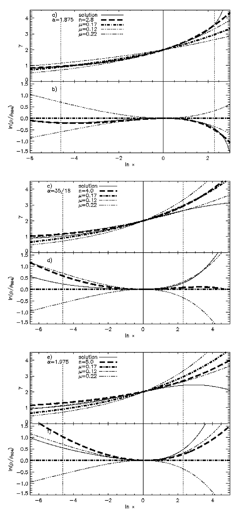
Figure 8: Solutions of Equation 10 with $\gamma^{\prime}(0)=1\times 10^{-5}$ (solid lines). The top plots in each panel show $\gamma$ distributions while the bottom panels present the corresponding density profiles normalized by the N04 distribution. The line types are the same in both plots. The thick dashed and dash-dotted lines correspond to Sérsic and N04 density distributions, respectively. The thin dash-dotted lines are Navarro et al. (2004) profiles with $\mu=0.12$; the thin dash-triple dotted lines have $\mu=0.22$. Note that the range of $\ln{(x)}$ is much smaller than in Figure 7; the vertical solid lines mark the positions of $r_{s}$ or $r_{2}$; the dotted vertical lines are 1/100 and 10 times this radius. In plots a and b, $\alpha=1.875$ and the Sérsic $n=2.8$. Plots b and c have ($\alpha=35/18,n=4.0$) and plots e and f have ($\alpha=1.975,n=5.0$).

The thin solid lines in Figure 8 are the $\gamma$ profiles for the solutions of Equation 10 with various $\alpha$ values and $\gamma^{\prime}(0)=1\times 10^{-5}$. The vertical solid lines denote the radius at which $\gamma=2$ and the dotted vertical lines mark $0.01$ and $10$ times this radius. Panel a in Figure 8 has $\alpha=1.875$. It is clear that the Sérsic form with $n=2.8$ provides a much better representation of the solution curve than do the Navarro et al. (2004) profiles. In panel b, $\alpha=35/18$ and the quasi-asymptotic behavior of the solution curve looks much more like one would expect for an NFW profile. However, an NFW $\gamma$ profile has a larger $\gamma^{\prime}(r_{s})$ than the solution curve and does not provide a good approximation. For this case, neither the Sérsic ($n=4.0$) nor the Navarro et al. (2004) curves are very good matches to the solution. The bottom panel shows the solution for $\alpha=1.975$. Again, the behavior of the solution curve is poorly represented by either the Sérsic ($n=5.0$) or Navarro et al. (2004) curves. The Sérsic behavior is not very surprising since Figure 4 shows that no Sérsic profile can produce $\alpha$ values as large as 1.975. While these last two plots point out the inadequacies of our fitting functions for general solutions of the constrained Jeans equation, in the case with $\alpha=1.875$, an average value from N-body simulations, the Sérsic profile provides a substanitally better fit over the N04 profile to the solution of the isotropic constrained Jeans equation.

5 Summary & Conclusions

The apparent commonness of power-law distributions in the phase-space density proxy $F\equiv\rho/\sigma^{3}\propto r^{-\alpha}$ (density divided by velocity dispersion cubed) in collapsed collisionless systems (e.g., Taylor & Navarro, 2001; Austin et al., 2005) has lead us to investigate 1) whether or not arbitrary equilibrium density profiles automatically lead to such behavior and 2) the types of equilibria that occur under the constraint that $F$ is scale-free. In this study, we have only investigated isotropic, spherically symmetric systems, but we will soon extend this work to include anisotropic distributions.

We find the $F$ distribution corresponding to the Hernquist (or King) profile is not an acceptable power-law and refutes the idea that mechanical equilibrium alone is responsible for power-law $F$ distributions. In general, profile types that empirically provide good fits to N-body halos produce power-law $F$ behavior, with the Navarro et al. (2004) and Sérsic types being superior to the generalized dual power-law profiles in this regard. We speculate that this ubiquity is not coincidence but rather that scale-free $F$ is a generic result of the physics of collisionless collapse. For the isotropic systems considered here, the Sérsic profile $F$ distributions with the smallest $\Delta_{\rm rms}$ values tend to have smaller $\alpha$ values than those corresponding to Navarro et al. (2004) profiles. However, each type of density profile covers the range of $\alpha$ values found in N-body simulations.

Taking power-law $F$ behavior as a given allows us to write a constrained Jeans equation that only involves the logarithmic density slope $\gamma$, its derivatives, and $\alpha$. This approach of deriving equilibrium density (actually, $\gamma$) distributions and comparing them to the $\gamma$ profiles corresponding to the Navarro et al. (2004) and Sérsic density profiles complements our earlier findings. The $\alpha=1.875$ results (top panel of Figure 8) echo our previous conclusions that N-body halos formed in cosmological simulations are best described by Sérsic models.

The preceeding points depend upon $\rho/\sigma^{3}$ vs. $r$ being the relevant relationship. As we do not have a compelling explanation for this relation, we have also investigated other correlations of $F$ with possibly more physical quantities. These quantities have so far failed to best the power-law correlation between $F$ and $r$. Another possibility is that $F$ itself is not the most illuminating variable. Based on a thoughful suggestion from R. Henriksen, we have also looked at whether or not the exponent of $\sigma$ in the combination $\rho/\sigma^{m}$ can be changed to produce a better power-law. Our results clearly point to $m=3$ as the most interesting value.

One other question to ask is whether or not any type of relaxation to equilibrium results in scale-free $\rho/\sigma^{3}$. In particular we have wondered what effect two-body relaxation may have. This is not to suggest that current N-body simulations are affected by two-body relaxation, but see El-Zant (2005). One argument against the importance of two-body relaxation in forming power-law $F$ is demonstrated by King profiles, which accurately model two-body relaxed globular clusters, but do not produce $F\propto r^{-\alpha}$. This is reminiscent of the findings of Binney (1982). That study found significant differences between de Vaucouleurs and King models’ $N(E)$ distributions ($N(E)dE$ is the number of particles with energies near $E$). Combining these findings with our own results for the King profile as well as the results of Austin et al. (2005) (halo formation without any two-body effects produces scale-free $F$) brings us to conclude that relaxation effects other than two-body interactions are responsible for the power-law $F$ distributions.

We have demonstrated that, in equilibrium, density profiles that accurately describe the end results of simulated collisionless collapses (and hence violent relaxation) produce power-law $F$ distributions, while those that have been designed mostly for analytical tractibility (e.g., Hernquist profiles) or to describe systems significantly different than galaxies (e.g., King models) do not. And though there is no general theory explaining power-law $F$ behavior, our findings encourage us to speculate that dynamical collapse processes (violent relaxation in particular) are playing a major role in making $\rho/\sigma^{3}$ of equilibrium systems scale-free.

References

- Ascasibar et al. (2004) Ascasibar, Y., Yepes, G., Gottlöber, S., Müller, V. 2004, MNRAS, 352, 1109
- Austin et al. (2005) Austin, C. G., Williams, L. L. R., Barnes, E. I., Babul, A., Dalcanton, J. J. 2005, accepted by ApJ, astro-ph/0506571
- Barnes et al. (2005) Barnes, E. I., Williams, L. L. R., Babul, A., Dalcanton, J. J. 2005, accepted by ApJ, astro-ph/0508160
- Bertschinger (1985) Bertschinger, E. 1985, ApJS, 58, 39
- Binney (1982) Binney, J. 1982, MNRAS, 200, 951
- Binney & Tremaine (1987) Binney, J., Tremaine, S. 1987, Galactic Dynamics, (Princeton:Princeton Univ. Press)
- Dalcanton & Hogan (2001) Dalcanton, J. J., Hogan, C. J. 2001, ApJ, 561, 35
- Dehnen & McLaughlin (2005) Dehnen, W., McLaughlin, D. E. 2005, astro-ph/0506528
- Diemand, Moore, & Stadel (2004a) Diemand, J., Moore, B., Stadel, J. 2004a, MNRAS, 352, 535
- Diemand, Moore, & Stadel (2004b) Diemand, J., Moore, B., Stadel, J. 2004b, MNRAS, 353, 624
- El-Zant (2005) El-Zant, A. A. 2005, astro-ph/0506617
- Graham et al. (2005) Graham, A. W., Merritt, D., Moore, B., Diemand, J., Terzić, B. 2005, astro-ph/0509417
- Hansen & Moore (2004) Hansen, S. H., Moore, B. 2004, astro-ph/0411473
- (14) Henriksen, R. private communication
- Hernquist (1990) Hernquist, L. 1990, ApJ, 356, 359