A necessary extension of the surface flux transport model

Customary two-dimensional flux transport models for the evolution of the magnetic field at the solar surface do not account for the radial structure and the volume diffusion of the magnetic field. When considering the long-term evolution of magnetic flux, this omission can lead to an unrealistic long-term memory of the system and to the suppression of polar field reversals. In order to avoid such effects, we propose an extension of the flux transport model by a linear decay term derived consistently on the basis of the eigenmodes of the diffusion operator in a spherical shell. A decay rate for each eigenmode of the system is determined and applied to the corresponding surface part of the mode evolved in the flux transport model. The value of the volume diffusivity associated with this decay term can be estimated to be in the range 50–100$\,\,\rm km^{2}\rm s^{-1}$ by considering the reversals of the polar fields in comparison of flux transport simulations with observations. We show that the decay term prohibits a secular drift of the polar field in the case of cycles of varying strength, like those exhibited by the historical sunspot record.

1 Introduction

Flux transport models describe the evolution of the flux distribution at the solar surface as a result of the emergence of bipolar magnetic regions and the transport of the corresponding radial magnetic flux by the horizontal flows due to convection, differential rotation and meridional circulation (e.g., Leighton, 1964; DeVore et al., 1984; Wang et al., 1989b; van Ballegooijen et al., 1998; Schrijver, 2001; Mackay et al., 2002; Durrant et al., 2004; Baumann et al., 2004). When applying the model to multiple solar cycles, Schrijver et al. (2002) and Wang et al. (2002) noticed that the secular evolution resulting from the simulations is not in agreement with the observations: activity cycles of varying strength lead to a drift of the polar fields and even to the disappearance of polar reversals.

The conceptual deficiency in the conventional flux transport models that leads to this disagreement with the observations arises from ignoring the vectorial nature and the radial structure of the magnetic field and, particularly, from omitting the part of the diffusion operator depending on the radial coordinate (see also Wilson et al., 1990; Dikpati & Choudhuri, 1994). This leads to an unwanted long-term memory of the surface flux since the decay time of a dipolar surface field increases strongly in the presence of a poleward meridional flow.

In order to avoid such unrealistic effects, Wang et al. (2002) made the assumption that the speed of the meridional flow is higher during more active cycles, while Schrijver et al. (2002) introduced an ad-hoc local decay term, calling upon the ‘sea-serpent’ flux emergence process combined with coronal field line reconnection as proposed by Spruit et al. (1987). Alternatively, Choudhuri & Dikpati (1999, and earlier references therein) have considered a consistent MHD model for the evolution of an axisymmetric field in the meridional plane of the Sun. Unfortunately, our understanding of the solar dynamo and the available computational resources are still insufficient to carry out such simulations in the three-dimensional case. We therefore suggest to extend the flux transport model by a modal version of the decay term proposed by Schrijver et al. (2002). We derive this term by considering the decay of the eigenmodes of the (volume) diffusion operator in a spherical shell. This leads to a consistent decay rate for each eigenmode, which can simply be incorporated in a code based upon expansion of the magnetic field into surface harmonics. The volume diffusion coefficient remains as a free parameter, which can be estimated by comparison of simulation results with observational constraints (like polar field reversals)

The outline of this paper is as follows. In Sect. 2 we determine the decay modes in a spherical shell for appropriate boundary conditions. The results are used in Sect. 3 to define the decay term extending the surface flux transport model. The value of the volume diffusivity (free parameter in the deacy term) is estimated by considering the evolution of the polar field over activity cycles of varying strength in Sect. 4 and by comparing the times of polar reversals with observational data in Sect. 5. We summarize our results in Sect. 6.

2 Decay modes of a poloidal field in a spherical shell

In the abscence of systematic flows, the time evolution of a magnetic field is described by the diffusion equation,

$$\frac{\partial\bf{B}}{\partial t}=-\eta\,\nabla\times(\nabla\times{\bf B})\,,$$ (1)

where $\eta$ is the (constant) magnetic diffusivity. In spherical geometry, the magnetic field vector can be written as the sum of a poloidal and a toroidal part, the latter having no radial component. Since the flux transport model assumes a purely radial magnetic field at the solar surface, it is sufficient to consider the decay of a poloidal magnetic field in a spherical shell (representing the solar convection zone), setting the non-radial components to zero at the outer boundary (the solar surface). The evolution of this field is described by Eq. (1), where $\bf{B}$ now represents a poloidal field. We introduce a spherical polar coordinate system with coordinates $(r,\theta,\phi)$, whose origin is located in the center of a sphere of radius $R_{\sun}$. The poloidal magnetic field can be represented by a scalar function, $S(r,\theta,\phi,t)$, as

$${\bf B}=-\nabla\times({\bf r}\times\nabla S)=-{\bf r}\,\triangle\;S+\nabla\frac{\partial}{\partial r}(rS)\,,$$ (2)

where $\triangle$ is the Laplace operator in spherical coordinates and r is the radius vector (Bullard & Gellman, 1954; Krause & Rädler, 1980) . Inserting this field representation into Eq. (1) we obtain

$$-\nabla\times\left({\bf r}\times\nabla\;\frac{\partial S}{\partial t}\right) = \eta\;\nabla\times\nabla\times\nabla\times\left({\bf r}\times\nabla S\right)$$ (3)

$$= \eta\;\nabla\times\nabla\times\left({\bf r}\times\triangle S\right)$$

$$= -\eta\;\nabla\times\left({\bf r}\times\nabla\triangle S\right)\,,$$

where we have used $\nabla\times{\bf r}=0$. From Eq. (3) it follows that

$${\bf r}\times\nabla\left[\eta\triangle S-\frac{\partial S}{\partial t}\right]=0\,.$$ (4)

The vector potential, $-{\bf r}\times\nabla S$, is invariant under gauge transformations, so that $S$ can be choosen such that the normalization condition

$$\int\limits_{-1}^{1}\int\limits_{0}^{2\pi}S\;d(\cos\theta)\;d\phi=0$$ (5)

is fulfilled for each value of $r$. Denoting by $\Omega$ the angular part of the spherical Laplace operator,

$$\triangle S = \frac{1}{r^{2}}\bigg{[}\frac{\partial}{\partial r}\left(r^{2}\frac{\partial S}{\partial r}\right)$$ (6)

$$+ \frac{1}{\sin\theta}\frac{\partial}{\partial\theta}\left(\sin\theta\frac{\partial S}{\partial\theta}\right)+\frac{1}{\sin\theta}\frac{\partial^{2}S}{\partial\phi^{2}}\bigg{]}$$

$$\equiv \frac{1}{r^{2}}\bigg{[}\frac{\partial}{\partial r}\left(r^{2}\frac{\partial S}{\partial r}\right)+\Omega S\bigg{]}\,,$$

we have

$$\int\limits_{-1}^{1}\int\limits_{0}^{2\pi}\Omega S\;d(\cos\theta)\;d\phi=0\;.$$ (7)

With the normalization condition, Eq. (5), we then find

$$\int\limits_{-1}^{1}\int\limits_{0}^{2\pi}\triangle S\;d(\cos\theta)\;d\phi=0\,.$$ (8)

Using this result, we obtain from Eq. (4) the scalar diffusion equation

$$\eta\triangle S-\frac{\partial S}{\partial t}=0\,.$$ (9)

We search for solutions of this equation within a spherical shell, $r_{\rm b}\leq r\leq R_{\sun}$, which are uniquely determined by specifying boundary conditions at the inner and outer boundaries. In accordance with the flux transport model, we assume the magnetic field to be radial at the surface. This leads to the boundary condition

$$\frac{\partial(rS)}{\partial r}=0\quad\quad\mbox{at}\quad r=R_{\odot}\,.$$ (10)

Table 1: Decay times $\tau_{ln}=1/(\eta\,k_{ln}^{2})$ (in years) for a volume diffusion coefficient of $\eta=100\,$km${}^{2}\,$s^-1. The modes are characterized by $l$, the number of node circles on spherical surfaces, and $n$, the number of nodes in the radial direction.

		$l$
		1	2	3	4	5	6	7	8	9
$n$	0	5.15	4.42	3.65	2.97	2.40	1.96	1.61	1.34	1.13
	1	0.62	0.60	0.58	0.56	0.53	0.50	0.47	0.44	0.41
	2	0.22	0.22	0.22	0.22	0.21	0.21	0.20	0.20	0.19
	3	0.11	0.11	0.11	0.11	0.11	0.11	0.11	0.11	0.10
	4	0.07	0.07	0.07	0.07	0.07	0.07	0.07	0.07	0.07

The bottom of the convection zone borders on the radiative core, which we represent by a field-free ideal conductor. Consequently, we require as boundary condition at $r=r_{\rm b}$ that the radial component of the magnetic field vanishes, which is equivalent to the condition

$$S=0\quad\quad\mbox{at}\quad r=r_{\rm b}\,.$$ (11)

In the numerical calculations below we take $r_{\rm b}=0.7R_{\sun}$, which corresponds to the bottom of the solar convection zone.

The general solution of Eq. (9) can be written as a decompostion into orthogonal decay modes (Elsasser, 1946),

$$S(r,\theta,\phi,t)=\sum_{n=0}^{\infty}\sum_{l=1}^{\infty}\sum_{m=-l}^{l}R_{ln}(r)\;Y_{lm}(\theta,\phi)\;T_{ln}(t)\,,$$ (12)

where we have omitted the monopole term ($l=0$). The functions $Y_{lm}$ are the spherical surface harmonics. Separation of variables leads to an exponential time dependence, viz.

$$T_{ln}(t)=\exp(-\eta\,k_{ln}^{2}t)\,,$$ (13)

where $1/\eta\,k_{ln}^{2}$ is the decay time of the mode characterized by the wave numbers $l$ and $n$. For the spherical harmonics we have

$$\triangle\;Y_{lm}(\theta,\phi)=-\frac{l\;(l+1)}{R^{2}_{\odot}}\;Y_{lm}(\theta,\phi)\,,$$ (14)

so that we obtain the following differential equation for the functions $R_{ln}(r)$:

$$r^{2}\frac{{\rm d}^{2}R_{ln}}{{\rm d}{r}^{2}}+2r\frac{{\rm d}R_{ln}}{{\rm d}{r}}+\bigg{[}k_{ln}^{2}{r}^{2}-l(l+1)\bigg{]}R_{ln}=0\,.$$ (15)

Solutions are the spherical Bessel functions of the first and second kind, $j_{l}$ and $y_{l}$, respectively, so that we have the general solution

$$R_{ln}(r)=a_{ln}\;j_{l}(k_{ln}r)+b_{ln}\;y_{l}(k_{ln}r)\,.$$ (16)

The linearity of the diffusion equation allows us to set the coefficients $a_{ln}$ to unity without loss of generality. The lower boundary condition, Eq. (11), is then used to determine $b_{ln}=-j_{l}(k_{ln}r_{\rm b})/y_{l}(k_{ln}r_{\rm b})$. Inserting this into Eq. (16) and using the upper boundary condition, Eq. (10), leads to

$$l\;\Big{[}j_{l}(k_{ln}R_{\sun})\;y_{l}(k_{ln}r_{\rm b})-j_{l}(k_{ln}r_{\rm b})\;y_{l}(k_{ln}R_{\sun})\Big{]}$$

$$\qquad-k_{ln}R_{\sun}\Big{[}j_{l-1}(k_{ln}R_{\sun})\;y_{l}(k_{ln}r_{\rm b})$$

$$\qquad\qquad\qquad-j_{l}(k_{ln}r_{\rm b})\;y_{l-1}(k_{ln}R_{\sun})\Big{]}=0\;,$$ (17)

from which the eigenvalues $k_{ln}$ can be determined numerically. The index $n$ is the number of nodes of the eigenfunction $R_{ln}(r)$ in $r_{\rm b}<r<R_{\sun}$. Note that the above construction shows that the eigenvalues, $k_{ln}$, and, therefore, the temporal decay rates of the eigenmodes do not depend on the azimuthal wave number, $m$, which describes the $\phi$-dependence of the mode.

Table 1 gives the decay times, $\tau_{ln}=1/(\eta\,k_{ln}^{2})$, in years for various modes, assuming a volume diffusion coefficient of $\eta=100\,$km${}^{2}\,$s^-1. The dipole mode ($l=1$) with $n=0$ has the longest decay time of about 5 years. While the decay times decrease only slowly for the higher multipoles (increasing $l$), the decay of the higher radial modes is much more rapid for the higher radial modes, being faster by a factor eight already for the mode $(l=1,n=1)$. It is therefore justified to consider only the most slowly decaying modes with $n=0$ in the decay term for the surface transport model.

3 Extension of the surface flux transport model

Figure 1: Evolution of the north (solid) and south polar fields (dashed) in the case of a systematic variation of strength between even and odd cycles for four values of $\eta$. Finite values of $\eta$ lead to stable oscillations of the polar fields while the field reversals (zero crossings) occur earlier with respect to the preceding activity minima (indicated by the dotted vertical lines.)

We use the results obtained in Sect. 2 to extend the surface transport model (DeVore et al., 1985; Wang et al., 1989a) by a decay term describing the volume diffusion of the poloidal magnetic field in the convection zone. This is certainly only a rough description of the evolution of the subsurface field, which can be improved once we have more quantitative information about the systematic flows in the deep convection zone. The working of the solar dynamo, on the other hand, is already represented in the model by the emergence of bipolar magnetic regions.

The extended equation for the evolution of the surface flux is written as

$$\frac{\partial B_{r}}{\partial t} = -\omega(\theta)\frac{\partial B_{r}}{\partial\phi}-\frac{1}{R_{\odot}\sin\theta}\frac{\partial}{\partial\theta}\bigg{(}v(\theta)B_{r}\sin\theta\bigg{)}$$ (18)

$$+ \frac{\eta_{\rm h}}{\mbox{\,$R_{\odot}$}^{2}}\left[\frac{1}{\sin\theta}\frac{\partial}{\partial\theta}\bigg{(}\sin\theta\frac{\partial B_{r}}{\partial\theta}\bigg{)}+\frac{1}{\sin^{2}\theta}\frac{\partial^{2}B_{r}}{\partial\phi^{2}}\right]$$

$$+ Q(\theta,\phi,t)-D(\eta)\,,$$

where $\omega(\theta)$ is the angular velocity of the photospheric plasma, $v(\theta)$ is the meridional flow velocity on the solar surface, $Q(\theta,\phi,t)$ is a source term describing the emergence of new magnetic flux, and $\eta_{\rm h}$ is the turbulent magnetic diffusivity associated with the nonstationary supergranular motions on the surface. We specify the decay term $D(\eta)$ on the basis of the decay modes in a spherical shell as determined in the previous section. To this end, we expand the instantaneous radial surface magnetic field into spherical harmonics,

$$B_{r}\left(\mbox{\,$R_{\odot}$},\theta,\phi,t\right)=\sum_{l=1}^{\infty}\sum_{m=-l}^{m=+l}c_{lm}(t)\;Y_{lm}\left(\theta,\phi\right)\,.$$ (19)

The volume diffusion leads to exponential decay of each of these modes with the corresponding decay times, $\tau_{ln}=1/(\eta\,k_{ln}^{2})$, depending on the radial structure of the magnetic field. Since the latter is unknown in the framework of the flux transport model, we only consider the mode $n=0$. This is justified by the fact that all higher modes ($n\geq 1$) decay much more rapidly (see Table 1), so that they do not affect the long-term, large-scale behaviour of the surface field that the flux transport models aim to describe. We therefore write $D(\eta)$ as

$$D(\eta)=\sum_{l=1}^{\infty}\sum_{m=-l}^{m=+l}\frac{c_{lm}(t)}{\tau_{l0}}\;Y_{lm}\left(\theta,\phi\right)\,.$$ (20)

As we have seen in Sect. 2, the decay times do not depend on the azimuthal wave number, $m$, of the mode. The modal decay term given by Eq.  (20) is particularly simple to implement in flux transport codes based upon an expansion into surface harmonics (e.g., van Ballegooijen et al., 1998; Mackay et al., 2002; Baumann et al., 2004).

The decay term, $D(\eta)$, depends on the turbulent volume diffusivity, $\eta$, which will generally differ from the diffusivity $\eta_{\rm h}$ related to the flux transport by the horizontal surface motions of supergranulation. Since the velocities and length scales of the dominant convective motions in the deep convection zone, which are relevant for $\eta$, are not well known, in the following sections we empirically estimate the value of $\eta$ by comparing with observed properties of the solar polar fields, namely the times of polar reversals and the sustained polar reversals in the case of solar cycles of varying strength.

4 Cycles of varying strength

One of the main problems with the original formulation of the flux transport model is the too long memory of the system. In the case of cycles with varying strength this can lead to a secular drift of the polar fields and a suppression of polar reversals. In the case of random fluctuations of the cycle amplitude, it results in a random walk of the polar fields superposed upon the cyclical variation. We illustrate this effects and their elimination through the decay term by way of a couple of examples.

Figure 2: Evolution of the north polar field (average above $75^{\circ}$ latitude) for a sequence of synthetic cycles with the flux emergence rate taken proportional to the sunspot numbers since 1700 (full line) and 1750 (dotted line), respectively, for different values of the volume diffusivity, $\eta$. The top panel ($\eta$=0) shows the strong drift of the polar field resulting from the secular increase of solar activity during the last century (see also Schrijver, 2001). Finite values of $\eta$ reduce the secular effect and lead to more symmetric variations, as observed; the volume diffusion term also largely removes the dependence of the results on the initial conditions (difference between full and dotted lines).

As a first illustration of the effect of the decay term introduced in the flux transport model, we consider simulations of synthetic sets of activity cycles (see Baumann et al., 2004, for a detailed description of the model) that vary systematically in strength: the cycle amplitudes (total amount of emergent flux) alternate by a factor of 2 between odd and even cycles. The results for the polar fields for several values of $\eta$ are shown in Fig. 1. We define the polar field, $B_{\rm pole}$, as the averaged radial field strength over the polar cap poleward of $75^{\circ}$ latitude. For $\eta=0$, i.e., in the absence of the added decay term, the polar fields show a strong secular drift (Fig. 1a). This results from the fact that, during the weaker cycles, the amount of opposite-polarity flux reaching the poles is insufficient to cancel the existing polar field and to build up a field of opposite polarity. This results in a systematic drift of the polar fields. Including the decay term leads to a shorter memory of the system and a stabilization of the oscillation (with some fluctuations due to the random component in the prescription of the flux emergence). For growing values of $\eta$, the drift of the polar fields ceases earlier and the asymmetry as well as the amplitude of the oscillation decreases (Fig. 1b–d). At the same time, the sign reversals of the polar fields occur earlier after the minima of flux eruption (activity minima, indicated by the dotted vertical lines) because the polar fields from the previous cycle have already been reduced by the effect of the decay term.

We have also considered the secular variation of solar activity in the historical record of sunspot numbers (see also Schrijver, 2001). Using the record of sunspot numbers since 1700, we have simulated a series of solar cycles with the flux transport code. We have used the ‘standard’ parameters (butterfly diagram of emerging bipolar regions, tilt angles, polarity rules, transport parameters, etc.) of Baumann et al. (2004), except for taking the emergence rate of the bipolar regions proportional to the sunspot numbers (monthly sunspot numbers since 1750 and monthly values interpolated from the yearly sunspot numbers before), thereby also using cycle lengths in agreement with the observed record. The overall free scaling factor for the flux emergence has been fixed by requiring that the total (unsigned) surface flux during the last three solar maxima (cycles 21–23) for the case $\eta=100\,\,\rm km^{2}\rm s^{-1}$ matches the observed values given by Arge et al. (2002). The evolution of the polar fields according to simulations with different values of $\eta$ is shown in Fig. 2. In order to evaluate the effect of the arbitrary initial condition (zero surface field) we also show a run starting from 1750, represented by the dotted line. In the case $\eta=0$ (no volume diffusion), the long memory of the system leads to a drift of the polar fields in the $20^{\rm th}$ century due to the secular increase of solar activity, so that the oscillations become very asymmetric, in striking contrast to the observed evolution of the polar fields. Finite values for $\eta$ of the order $100\,\,\rm km^{2}\rm s^{-1}$ lead to more symmetric oscillations and a suppression of the unrealistic drift. The amplitude of the simulated polar field in the last cycles for a value of $\eta=100\,\,\rm km^{2}\rm s^{-1}$ is roughly consistent with the published observational data, which indicate amplitudes for the field strength of 10–20 G (e.g., Wang & Sheeley, 1995; Arge et al., 2002; Dikpati et al., 2004; Durrant et al., 2004). Comparing the two runs with different starting times (full line and dotted line), we find that the long memory of the system in the case $\eta=0$ leads to a significant difference between these two runs. For $\eta\neq 0$, on the other hand, there is almost no dependence on the initial condition after a few cycles.

5 Polar field reversal times

Table 2: Epochs of reversals (average of north and south pole) of the simulated polar magnetic field poleward of $\pm 75^{\circ}$ latitude for three values of the magnetic volume diffusivity, $\eta$ (in $\,\rm km^{2}\rm s^{-1}$), in comparison with the reversal times inferred by Makarov et al. (2003) on the basis of polar crown filaments, $T_{\rm c}$, and from H$\alpha$ synoptic charts, $T_{\rm l=1}$. The row at the bottom gives the average time intervals (in years) between the reversals and the preceding sunspot minima ($T_{\rm min}$, last column).

Cycle #	$\eta=50$	$\eta=100$	$\eta=200$	$T_{\rm c}$	$T_{\rm l=1}$	$T_{\rm min}$
13	1895.0	1893.7	1892.7	1895.0	1893.2	1889.6
14	1907.8	1906.7	1905.2	1908.7	1905.8	1901.7
15	1918.4	1917.5	1916.4	1918.7	1916.3	1913.6
16	1928.9	1927.7	1926.8	1929.9	1927.0	1923.6
17	1938.2	1937.7	1936.8	1940.1	1936.5	1933.8
18	1949.5	1948.4	1947.3	1950.2	1947.3	1944.2
19	1958.6	1957.9	1957.1	1959.7	1957.2	1954.3
20	1971.6	1969.6	1968.3	1971.5	1968.6	1964.9
21	1981.2	1980.6	1979.6	1981.8	1979.9	1976.5
22	1991.3	1990.6	1989.7	1991.8	1990.4	1986.8
23	2002.3	2001.3	1999.8	2001.7	1999.7	1996.4
$\langle T_{\rm rev}-T_{\rm min}\rangle$	$5.2\pm 0.8$	$4.2\pm 0.5$	$3.1\pm 0.2$	$5.8\pm 0.6$	$3.3\pm 0.5$

Having shown that the decay term prohibits drifts and an unrealistic long-term memory of the polar fields for values of $\eta$ of the order of $100\,\,\rm km^{2}\rm s^{-1}$, we now consider its effect on the calculated reversal times of the polar fields and compare quantitatively with observational results.

Figure 3: Synthetic solar cycles: dependence on $\eta$ of the (a) averaged unsigned surface field (maxima and minima, respectively), (b) the maxima of the polar polar field, and (c) the polar reversal times after the previous activity minimum (minimum of the cyclic flux emergence rate in the model).

5.1 Synthetic cycles

In order to illustrate the effect of the decay term on the reversal times, we consider synthetic cycles of equal strength and determine the reversal times of the polar field in dependence on the value of $\eta$. In addition, we also consider the averaged (unsigned) field over the whole surface, $B_{\rm tot}$, and the maximum polar field during a cycle. The absolute values of the field strength are arbitrary; here we are only concerned with the dependence on $\eta$. Fig. 3 shows: $B_{\rm tot}$ for cycle maxima and minima, respectively (Fig. 3a), the maximum polar field (Fig. 3b), and the reversal time in years after the previous flux emergence (activity) minimum (Fig. 3c), all as functions of $\eta$.

While the average surface field during cycle maxima varies only slightly with $\eta$, there is a somewhat stronger decline of the values during cycle minima (Fig. 3a), similar in proportion to the decline of the maximum polar field with increasing $\eta$ (Fig. 3b). This results from the fact that, during activity minimum, both the polar and the total field are dominated by the dipole mode, which suffers from enhanced decay due to volume diffusion. A strong effect of the value of $\eta$ on the polar reversal times is clearly visible in the lower panel. For increasing $\eta$, the reversals occur earlier after cycle minimum, varying between 5.1 years for $\eta=0$ and 2.8 years for $\eta=200\,\rm km^{2}\rm s^{-1}$. This results from the stronger decay of the polar field from the previous cycle, so that less opposite-polarity flux of the new cycle is required to reverse the field, leading to an earlier reversal time.

Although these synthetic cycles are not intended for a quantitative comparison with actual solar data since they do not include a long-term modulation of the cycle amplitudes and also no variation of the cycle length, we may nevertheless check whether they are roughly consistent with the data. Makarov et al. (2003) used two different methods to determine polar reversal times for the period 1878–2001: (1) by the disappearance of the polar crown filaments, and (2) from estimating the magnetic dipole configuration on the basis of H$\alpha$ synoptic charts. They find that reversals occur on average 5.8 years after the previous sunspot minimum for method (1) while they obtained a value of 3.3 years with method (2). Makarov et al. (2003) consider the first method to be more reliable. On the other hand, the magnetograph data compiled by Arge et al. (2002) and Dikpati et al. (2004) for the the solar cycles 21–23 indicate an average reversal time about 4.6 years after sunspot minimum, about the mean of the two values given by Makarov et al. (2003). Comparing this with the bottom panel of Fig. 3, we find that a value of $\eta$ in the range 50–100$\,\,\rm km^{2}\rm s^{-1}$ leads to reversal times that are consistent with these results. A quantitatively more reliable comparison is carried out in the subsequent section.

5.2 Simulation of solar cycles No. 13 – 23 on the basis of RGO/SOON sunspot data

For a quantitative comparison with observations, we determine the magnetic flux input into the flux transport model on the basis of the sunspot group areas from the digitized version of the Royal Greenwich Observatory (RGO) photographic results, which are available for the time period 1874-1976. For the time after 1976, this series is continued by data from the Solar Optical Observing Network (SOON) of the US Air Force. We have combined both datasets and transformed them into a sequence of emerging active regions. Below we give a brief summary of the procedure; a more detailed description will be given elsewhere.

We take each observed sunspot group to provide a bipolar magnetic region and determine its total unsigned magnetic flux from the observed sunspot area and an associated facular (plage) area according to the empirical relationship derived by Chapman et al. (1997). We use the sunspot groups in the databases at the time of their maximum area development, thus ensuring that every group is considered only once. Furthermore, we take only sunspot groups that reach their maximum area within $\pm 45^{\circ}$ of the central meridian. Owing to the large number of observations, we consider this $90^{\circ}$ window to be representative for the whole sun. In order to roughly account for the flux emergence on the full solar surface, we copy this $90^{\circ}$ window three times into the remaining $270^{\circ}$ longitude range. Each of the sunspot groups determined in this way provides a bipolar magnetic region whose orientation of the magnetic polarities is assigned according to Hales’ polarity rules and whose tilt angle, $\alpha$, is assumed to be given by Joy’s law, i.e. $\alpha=0.5\,\lambda$, where $\lambda$ is the latitude. Further details about the treatment of bipolar magnetic region are given in Baumann et al. (2004). The overall scaling factor in the magnetic flux of the emerging bipolar regions is chosen such that the flux transport simulations reproduce the evolution of the observed total surface field given by Arge et al. (2002) and the polar field strengths given by Dikpati et al. (2004).

We have carried out a flux transport simulation based upon the set of input data covering the period 1874–2005. For the interval 1974–2005, the time-latitude diagrams of the longitudinally averaged magnetic field from the simulation can be compared with the corresponding diagram derived by D. Hathaway (NASA/Marshall Space Flight Center) from the NSO/Kitt Peak synoptic maps. Fig. 4 shows this comparison for three values of the volume diffusivity: $\eta=0,\,100,\,200\,\rm km^{2}\rm s^{-1}$. The evolution of the global field is best reproduced by the case $\eta=100\,\rm km^{2}\rm s^{-1}$, which yields the nearest agreement of the reversal times of the polar fields for the last three cycles.

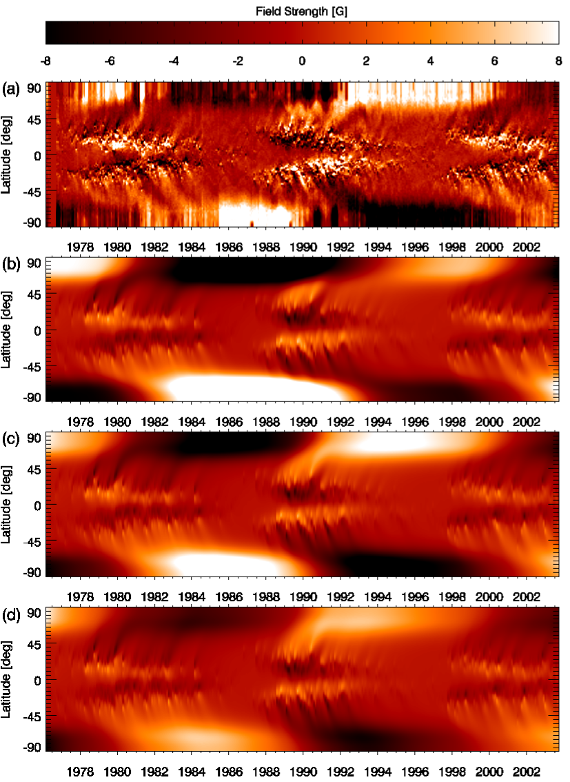
Figure 4: Comparison between observed magnetic field distribution from 1974 on (panel a, based upon NSO/Kitt Peak data, courtesy D. Hathaway) and flux transport simulations for different values of the volume diffusivity: $\eta=0$ (panel b), $\eta=100\,\rm km^{2}\rm s^{-1}$ (panel c), and $\eta=200\,\rm km^{2}\rm s^{-1}$ (panel d). Shown are time-latitude diagrams of the longitudinally averaged surface field. The simulations reproduce the global development of the magnetic field, with poleward surges of following-polarity flux leading to reversal of the polar fields around sunspot maxima. However, in the case without the decay term (panel b), the reversals occur too late. For non-vanishing values of $\eta$, the reversal times are shifted forward in time; the best agreement with the observed reversal times is obtained for $\eta=100\,\rm km^{2}\rm s^{-1}$ (panel c).

In order to compare with the result of Makarov et al. (2003), we have determined the epochs of the reversals of the average field poleward of $\pm 75^{\circ}$ latitude from the flux transport simulations for the solar cycles 13–23. The reversal times (average of the north and south polar reversals) are given in Table 2 together with the reversal times inferred by Makarov et al. (2003) from the evolution of polar-crown filaments ($T_{\rm c}$) and from H$\alpha$ synoptic charts ($T_{\rm l=1}$), respectively. The last row gives the average time interval (in years) between the polar reversal and the preceding solar minimum. We recover the trend towards earlier reversals for larger values of $\eta$ found in the previous section for the synthetic cycles. The values cover about the range defined by the results from the two methods used by Makarov et al. (2003). However, even with $\eta=50\,\rm km^{2}\rm s^{-1}$ we do not reach the value of 5.8 years that they determined from the disappearance of polar crown filaments. This could be due to the fact that we define the polar reversal from the average field in the caps poleward of $\pm 75^{\circ}$ latitude, while the polar crown filaments probably disappear later, when the last remnant of the old polarity in fact vanishes. A fair degree of averaging is also inherent in the magnetograph data shown by Dikpati et al. (2004), from which we roughly estimate an average reversal time of 4.6 years after sunspot minimum. Altogether, we conclude that a volume diffusivity in the range 50–100 $\,\rm km^{2}\rm s^{-1}$ is probably adequate for flux transport models of the solar surface field. This is also consistent with the timings of the polar reversals with respect to the sunspot maxima: for $\eta=50\,\rm km^{2}\rm s^{-1}$ the polar field reverse on average 1.3 years after solar maximum; for $\eta=100\,\rm km^{2}\rm s^{-1}$ we find an average value of 0.3 years after maximum.

6 Conclusion

We have shown that a modified (modal) version of the decay term first introduced into the flux transport model by Schrijver et al. (2002) can be derived consistently from the volume diffusion process that is (among other factors) neglected in the standard flux transport models. Including this term removes the unrealistic long memory of the system and thus prohibits a secular drift or a random walk of the polar fields in the case of activity cycles with variable amplitude. The value of the (turbulent) magnetic volume diffusivity, $\eta$, can be estimated by considering the reversal times of the polar field relative to the preceding activity minimum and by comparing with direct observations or values inferred from proxy data. We find that values of $\eta$ in the range 50–100$\,\,\rm km^{2}\rm s^{-1}$ are consistent with the observational constraints. This is also the order of magnitude suggested by simple estimates based on mixing-length models of the convection zone. With this consistent extension and improvement of the model, flux transport simulations of the large-scale magnetic field on the solar surface over many activity cycles can be carried out.