High-energy Cosmic Rays

Abstract

After a brief review of galactic cosmic rays in the GeV to TeV energy range, we describe some current problems of interest for particles of very high energy. Particularly interesting are two features of the spectrum, the knee above $10^{15}$ eV and the ankle above $10^{18}$ eV. An important question is whether the highest energy particles are of extra-galactic origin and, if so, at what energy the transition occurs. A theme common to all energy ranges is use of nuclear abundances as a tool for understanding the origin of the cosmic radiation.

1 Introduction

The cosmic-ray spectrum falls steeply, decreasing by approximately a factor of 50 per decade increase in energy when plotted as $E\phi(E)=dN/d\ln(E)$. In the lowest energy region the flux is high enough so that the elemental composition of the primary cosmic-ray nuclei can be studied by direct observations with detectors lifted above the atmosphere by balloons or spacecraft. In the GeV range, even individual isotopes can be resolved. In this lower energy range we have the most detailed information on which to base a model of the origin of cosmic rays.

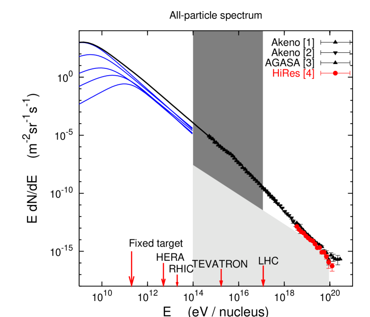
Figure 1: Summary of the cosmic-ray spectrum. The five lines below 100 GeV indicate the individual contributions of five individual groups of nuclei (protons, helium, CNO, Mg-Si and Fe). For clarity only subsets [1, 2, 3, 4] of the data are shown.

Above $10^{14}$ eV, where the flux falls below several particles per square meter per day, direct measurements of the primaries are no longer practical. On the other hand, this energy is large enough so that secondary cascades penetrate with a footprint large enough to be measured by an array of detectors on the ground. Such an extensive air shower (EAS) array typically has dimensions of a fraction of a square kilometer or more and can be operated for years rather than days or weeks. An EAS experiment in effect uses the atmosphere as a calorimeter, so the showers are classified by total energy per particle rather than by energy per nucleon as at low energy. Because of the sparse quality of the information, however, the energy per shower is only determined with relatively large uncertainty, and the best one can do is to determine the relative contributions of groups of elements. The situation is exacerbated by large shower-to-shower fluctuations coupled with less than full knowledge of the properties of the hadronic interactions that govern shower development. The latter problem becomes more severe in the highest energy range, which is beyond the reach of current accelerators.

Figure 1 is a schematic plot of the cosmic-ray spectrum as a function of total energy per nucleus. The plot is divided into three regions by the shading. The relatively detailed measurements of spectra of individual elements (or groups of elements) below $10^{14}~{}eV$ supports a fairly well-developed model of the origin of these particles. In particular, the observed energy density and propagation time of the cosmic-rays together determine the power required by the sources. This connection suggests an approach that may be helpful in understanding the origin of the higher energy particles. The second region (dark shading) includes the knee where there is a steepening and perhaps some structure in the spectrum that needs explanation. The highest energy region includes the ankle, a flattening of the spectrum above $10^{18}$ eV that may be related to a transition from particles of galactic origin to those accelerated in extra-galactic sources. The question of whether there is a transition to cosmic rays of extra-galactic origin, and if so where it occurs, is of considerable interest. Finally, the question of whether the spectrum extends beyond $10^{20}$ eV is currently the foremost problem in high-energy particle astrophysics because of the difficulty of accounting for the absence of energy loss by protons in the microwave background radiation if the spectrum is not suppressed above this energy.

In what follows we discuss the three energy regions in order. A common theme is use of the primary composition as a clue to the nature of the sources of the particles.

2 Galactic cosmic rays $E\,<\,10^{14}$ eV

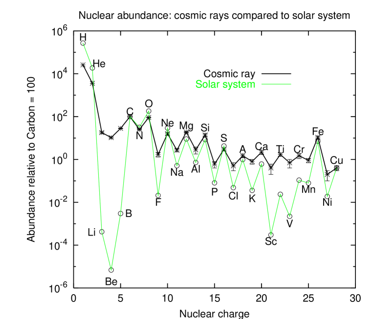
Figure 2: Comparison of Solar system [9] and cosmic-ray elemental abundances. Nuclear abundances are from [10]; protons and helium are from [11, 12].

A classic problem in nuclear astrophysics is the determination of the cosmic-ray source abundances [5, 6]. This requires a model of the galaxy, including the spatial distribution of cosmic-ray sources; density, composition and ionization state of the interstellar medium; and the strength and topology of the magnetic field. Important recent investigations of cosmic-ray propagation from two different viewpoints may be found in Refs. [7] and [8]. Here we give only the main points in a simplified form. The starting point is a determination of the abundances of different nuclei near the solar system (but outside the heliosphere). Figure 2 shows the elemental abundances in the cosmic radiation. The overabundance by several orders of magnitude of secondary elements such as lithium, beryllium and boron relative to their general abundance in solar system material is a consequence of spallation of the more abundant primary nuclei, especially carbon and oxygen. A similar situation occurs for the secondary nuclei just below iron.

Given a knowledge of the spallation cross sections, one has to solve a set of coupled propagation equations for the diffusion of the cosmic-rays in the turbulent, magnetized interstellar medium. A simplified version of the relevant set of equations is

$${N_{i}(E)\over\tau_{esc}(E)}\,=\,Q_{i}(E)-\left(\beta cn_{H}\sigma_{i}+{1\over\gamma\tau_{i}}\right)N_{i}(E)+\beta cn_{H}\sum_{k\geq i}\sigma_{k\rightarrow i}\,N_{k}(E).$$ (1)

Here $N_{i}(E)$ is the spatial density of cosmic-ray nuclei of mass $i$, and $n_{H}$ is the number density of target nuclei (mostly hydrogen) in the interstellar medium, $Q_{i}(E)$ is the number of primary nuclei of type $i$ accelerated per cm³ per second, and $\sigma_{i}$ and $\sigma_{k\rightarrow i}$ are respectively the total and partial cross sections for interactions of cosmic-ray nuclei with the gas in the interstellar medium. The second term on the r.h.s. of Eq. 1 represents losses due to interactions with cross section $\sigma_{i}$ and decay for unstable nuclei with lifetime $\tau_{i}$.

Essentially, in the simplest diffusion model, the secondary to primary ratios determine the product of density of the interstellar medium times the characteristic propagation time of cosmic-rays before they escape from the Galaxy ($\tau_{esc}$). This can be seen by solving Eq. 1 for a secondary nucleus $S$ while neglecting its losses during propagation and assuming that $Q_{S}\approx 0$. Representing the parent primary nuclei by a single contribution $N_{P}$ then leads to a simplified equation

$${m_{p}\over\sigma_{P\rightarrow S}}\,{N_{S}\over N_{P}}\;=\;\rho\,\beta\,c\,\tau_{esc}\;\approx\;5\;{\rm g/cm}^{2}.$$ (2)

The approximate value given in Eq. 2 requires accounting for several terms with appropriate spallation cross sections for its derivation from the data. The numerical value in Eq. 2 would imply $\tau_{esc}\,\approx\,3\times 10^{6}$ years if the average density $\rho$ corresponds to one hydrogen atom per cubic centimeter as in the disk of the galaxy.

Two details of the data are particularly important. One is the ratio $R_{10}$ of the unstable isotope ¹⁰Be to stable ⁹Be. ¹⁰Be is unstable to $\beta$-decay with a half-life of $\tau_{10}\;=\;1.5\times 10^{6}$ years. The two isotopes of beryllium are produced in comparable amounts by spallation of heavier nuclei. If $R_{10}$ as measured is comparable to the production ratio, then $\tau_{esc}\ll\tau_{10}$; if $R_{10}\sim 0$ then $\tau_{esc}\gg\tau_{10}$. The data indicate

$$\tau_{esc}\approx 2\times 10^{7}\;{\rm years}.$$ (3)

Given the mean density of the interstellar medium, the relatively large value of $\tau_{esc}$ implies that cosmic ray nuclei spend significant time diffusing in low-density regions, possibly above the gaseous disk in the galactic halo, before escaping into inter-galactic space.

The other significant feature is that the ratio of secondary to primary nuclei decreases with increasing energy. From Eq. 2 this implies that $\tau_{esc}$ decreases with energy. This behavior is attributed to energy-dependent diffusion, whereby higher energy particles diffuse out of the galaxy more quickly than those of lower energy. It should apply to all cosmic rays, including primary protons, as well as secondary nuclei if the model is consistent and complete. The observed primary spectrum $\phi(E)$ and the source spectrum $Q(E)$ are connected by a relation of the form

$$\phi(E)\;=\;Q(E)\times\tau_{esc}(E).$$ (4)

A simple power-law fit to available data gives

$$\tau_{esc}(E)\;\propto\;E^{-\delta}$$ (5)

with $\delta\approx 0.6$. Since the observed differential energy spectrum is proportional to $E^{-2.7}$, the inferred source spectrum would be $\propto\,E^{-2.1}$.

An inferred spectral index at the source of -2.1 is often cited as evidence for first order diffusive shock acceleration, which, in the test-particle approximation predicts a value of -2.0. The situation is actually more complicated. On the one hand, the relation 5 cannot hold over a large energy range without coming in conflict with the observed isotropy of high-energy cosmic-rays. Extrapolating Eq. 5 to $10^{15}$ eV, for example, would lead to a value of $\tau_{esc}$ almost as small as the light travel time across the galactic disk, implying a larger anisotropy than is observed. On the other hand, a more complete treatment of shock acceleration that accounts for the non-linear back-reaction of the accelerated particles on the shock structure [13], gives a somewhat concave energy spectrum rather than a single power law (i.e. steeper spectrum at low energy, hardening at high energy). Models in which some of the energy-dependence of the secondary/primary ratio is attributed to reacceleration [14] during propagation can accommodate a somewhat steeper average source spectrum and correspondingly a larger value of $\tau_{esc}$ at high energy, more consistent with the observed small anisotropy. One possibility is that the observed average spectrum is a composite of contributions from many individual sources having a range of individual properties. In what follows, for illustration we assume $Q(E)\propto E^{-2.4}$ in which case $\delta\approx 0.3$.

The next step is to estimate the power required of the sources to maintain the observed spectrum in equilibrium. The total source power is related to the locally observed energy spectrum by

$$\int\,Q(E)\,{\rm d}E\;=\;{4\pi\over c}\,\int\,E\,{\phi(E)\over\tau_{esc}(E)}\,{\rm d}E.$$ (6)

The pre-factor on the r.h.s. of this equation converts the measured cosmic-ray flux $\phi$ to the corresponding spatial density of cosmic rays. Fixing $\tau_{esc}$ in the GeV range according to Eq. 3 and evaluating the integral using the measured spectrum and Eq. 5 for $\tau_{esc}$ leads to an estimate of the source power as $\sim 10^{-26}$ erg cm^-3s^-1. If the flux observed locally near the solar system is typical of the galactic disc, then the total power of the cosmic-ray sources is obtained by multiplying by the volume of the disk, $\sim 10^{67}$cm³, for an estimate of $10^{41}$ erg/s. The average power generated in kinetic energy of ejected material (exclusive of neutrinos) in galactic supernova explosions is $\sim 10^{42}$ erg/s ($10^{51}$ erg/30 year).

The combination of an acceleration theory which produces approximately the right spectrum with high efficiency (first order diffusive shock acceleration) and a source with the right power makes supernova shock acceleration a favored candidate for the origin of cosmic rays in the galaxy. From observations of synchrotron radiation, it is possible to see direct evidence of electrons being accelerated to high energy in individual supernova remnants [15]. What has proved more difficult is to find examples of individual supernova remnants in which acceleration of protons can be verified by the production of neutral pions [16]. The problem is that it is usually possible to explain the observed electromagnetic radiation as radiation from energetic electrons, by bremsstrahlung at lower energy and by inverse Compton scattering at higher energy. The characteristic kinematic signature of pion production (a peak at a photon energy of half the pion mass) tends to be obscured by superimposed synchrotron and bremsstrahlung photons [17]. Indirect arguments related to the shape of the observed gamma-ray spectrum above a TeV can in some cases most easily be accounted for if the source is production of $\pi^{0}$ by protons rather than radiation by electrons [18]. A nice review of models of galactic cosmic ray sources is Ref. [19].

Observation of neutrinos from SNR (or any other potential cosmic accelerator) would be conclusive evidence for acceleration of primary protons because only hadronic processes can produce neutrinos. The expected fluxes are low, however, so large detectors will be needed to detect them [20].

3 The knee: $10^{14}<E<10^{17}$ eV

Diffusive shock acceleration works to the extent that charged particles gain energy by an amount $\Delta E$ proportional to $E$ each time they cross from upstream to downstream and back upstream of the shock. (Here upstream is the unshocked region and $E$ is the energy before adding the increment $\Delta E$.) After a time $T$ the maximum energy achieved is

$$E_{max}\;\sim\;Ze\beta_{s}\times B\times T\,V_{s},$$ (7)

where $\beta_{s}=V_{s}/c$ refers to the velocity of the shock. This result is an upper limit in that it assumes a minimal diffusion length equal to the gyroradius of a particle of charge $Ze$ in the magnetic field $B$ upstream of the shock. Using numbers typical of Type II supernovae exploding in the average interstellar medium gives $E_{max}\sim Z\times 100$ TeV [21]. More recent estimates give a maximum energy larger by as much as order of magnitude or more for some types of supernovae [22].

The nuclear charge, $Z$, appears in Eq. 7 because acceleration depends on the interaction of the particles being accelerated with the moving magnetic fields. Particles with the same gyroradius behave in the same way. Thus the appropriate variable to characterize acceleration is magnetic rigidity, $R\,=\,pc/Ze\,\approx E_{tot}/Ze$, where $p$ is the total momentum of the particle. Diffusive propagation also depends on magnetic fields and hence on rigidity. For both acceleration and propagation, therefore, if there is a feature characterized by a critical rigidity, $R^{*}$, then the corresponding critical energy per particle is $E^{*}\,=\,Z\times R^{*}$.

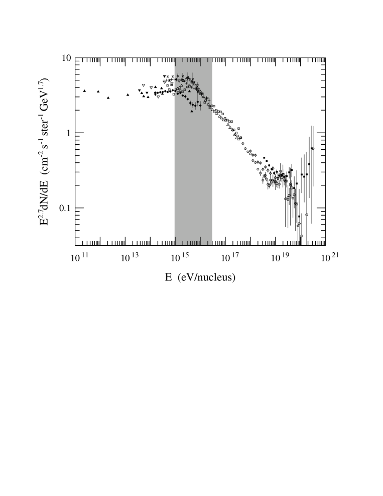
Figure 3: High-energy cosmic-ray spectrum. References to the data are given in [23]. The shaded region indicates a factor a 30 in total energy (see text).

The knee of the spectrum is the steepening that occurs above $10^{15}$ eV, as shown in Fig. 3, while the ankle is the hardening around $3\times 10^{18}$ eV. One possibility is that the knee is associated with the upper limit of acceleration by galactic supernovae, while the ankle is associated with the onset of an extragalactic population that is less intense but has a harder spectrum that dominates at sufficiently high energy. A generic two-component model was suggested long ago by Peters [24], but this explanation does not fit the data, at least not in its simplest form.

Consider first the situation if all galactic sources accelerated particles to the same maximum rigidity, say $10^{15}$ V. Then, since the abundant nuclei are in the range $1\leq Z\leq 26$, the spectrum would be expected to cutoff altogether within a factor of about $30$ as a consequence of the prefactor $Z$ in Eq. 7. The protons would cut off first, followed by helium then CNO, etc. [24]. The range over which the cutoff would occur is indicated by the shaded region in Fig. 3. Clearly, this is not at all what happens. Instead, the spectrum continues smoothly for another two decades in energy. Even postulating a significant contribution from elements heavier than iron (up to uranium [25]) cannot explain the smooth continuation all the way up to the ankle.

One possibility is that most galactic accelerators cut off around a rigidity of perhaps $10^{15}$ eV, but a few accelerate particles to much higher energy and account for the region between the knee and the ankle [26]. This scenario would be a generalization of Peters’ model. Its signature would be a sequence of composition cycles alternating between light and heavy dominance as the different components from each source cut off. As emphasized by Axford [27], however, the problem with this type of model is that it requires a fine-tuning of the high-energy spectra so that they rise to join smoothly at the knee then steepen to fit the data to $\sim 10^{18}$ eV. As a consequence, several models have been proposed in which the lower-energy accelerators ($E\,<\,10^{15}$ eV) inject seed particles into another process that accelerates them to higher energy. In this way the spectrum above the knee is naturally continuous with the lower energy region. Groups of supernovae [27] and a termination shock in the galactic wind [28] have been suggested [29].

The fine tuning problem (i.e. to achieve a smooth spectrum with a sequence of sources with different maxima) was actually clearly recognized by Peters in his original statement of this idea [24]. He correctly point out, however, that since the cutoff is a function of rigidity while the events are classified by a quantity close to total energy, the underlying discontinuities are smoothed out to some extent. An interesting question to ask in this context is what source power would be required to fill in the spectrum from the knee to the ankle. The answer depends on what is assumed for the spectrum of the sources and the energy dependence of propagation in this energy region. Reasonable assumptions (e.g. $Q(E)\propto E^{-2}$ and $\tau_{esc}\propto E^{-\delta}$ with $\delta\approx 0.3$) lead to an estimate of $\sim 2\times 10^{39}$ erg/s, less than 10% of the total power requirement for all galactic cosmic-rays. For comparison, the micro-quasar SS433 at 3 kpc distance has a jet power estimated as $10^{39}$ erg/s [30].

Another possibility is that the steepening of the spectrum at the knee is a result of a change in properties of diffusion in the interstellar medium such that above a certain critical rigidity the characteristic propagation time $\tau_{esc}$ decreases more rapidly with energy. If the underlying acceleration process were featureless, then the relative composition as a function of total energy per particle would change smoothly, with the proton spectrum steepening first by $0.3$, followed by successively heavier nuclei. It is interesting that this possibility was also explicitly recognized by Peters [24].

A good understanding of the composition would go a long way toward clarifying what is going on in the knee region and beyond. A recent summary of direct measurements of various nuclei shows no sign of a rigidity-dependent composition change up to the highest energies accessible ($\sim 10^{14}$ eV/nucleus) [31]. The change associated with the knee is in the air shower regime. Because of the indirect nature of EAS measurements, however, the composition is difficult to determine unambiguously. The composition has to be determined from measurements of ratios of different components of air showers at the ground. For example, a heavy nucleus like iron generates a shower with a higher ratio of muons to electrons than a proton shower of the same energy. The best indication at present comes from the Kascade experiment [32], which shows clear evidence for a “Peters cycle”, the systematic steepening first of hydrogen, then of helium, then CNO and finally the iron group. The transition occurs over an energy range from approximately $10^{15}$ eV to $3\times 10^{16}$ eV, as expected, but the experiment runs out of statistics by $10^{17}$ eV, so the data do not yet discriminate among the various possibilities for explaining the spectrum between the knee and the ankle.

4 The ankle: $E>10^{17}$ eV

The energy range above 10¹⁷ is where a transition from cosmic rays accelerated in the Galaxy to cosmic rays from extra-galactic sources may be expected. The gyroradius of 10¹⁹ eV protons is of order 10 kpc, exceeding the dimensions of the inner Galaxy. Such particles could not be contained in the Galaxy [33], not to mention the difficulty of accelerating particles to such high energy with known potential galactic accelerators. The spectrum of the highest energy cosmic rays indeed shows an ‘ankle’ around $3\times 10^{18}$ eV where the power law spectrum flattens to a differential index of about $2.7$. One possibility is that this feature itself reflects the transition to dominance of extragalactic cosmic rays. Another possibility is that particles of extragalactic origin become the dominant population at lower energy and that the ankle is a feature due to energy loss of protons to electron-positron pair production on the microwave background during propagation [34].

What is needed to decide the question is knowledge of the composition as a function of energy. The idea is that in the range where the last galactic accelerator reaches its upper limit the composition will start changing in the same way as it does at the ‘knee’. In an energy range of about one and a half decades the composition should change from one dominated by protons and light nuclei to heavy nuclei, signaling the upper limit of Galactic sources. As the extragalactic population of particles begins to dominate, the composition should change back toward lighter nuclei, assuming the extragalactic cosmic rays consist primarily of protons.

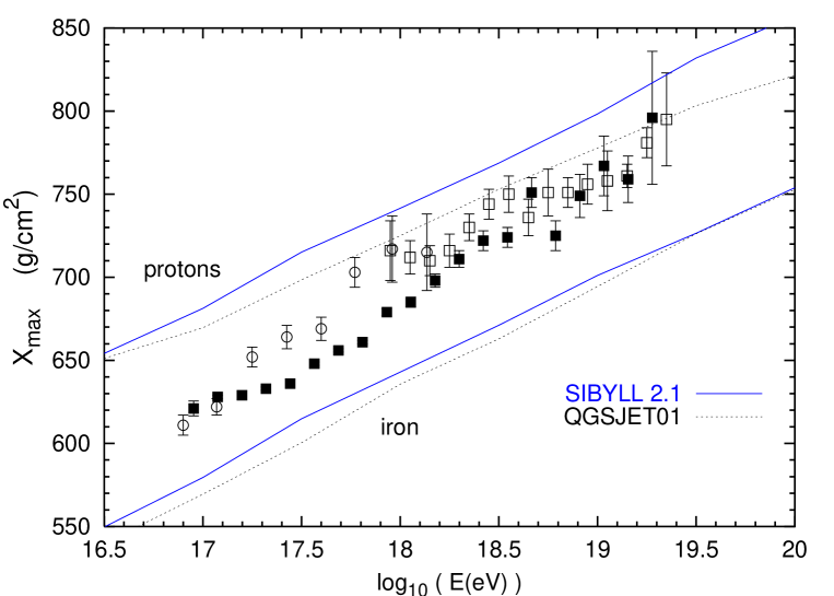
Figure 4: Plot of data on mean depth of maximum vs energy. Filled squares are data from the stereo Fly’s Eye [39]. Open symbols show the data of HiRes (squares) and HiRes prototype with MIA (circles) [40].

In this energy range the composition is measured by the energy dependence of the position of shower maximum, $X_{max}$. An air shower consists of a superposition of electromagnetic cascades initiated by photons from decay of $\pi^{0}$ particles produced by hadronic interactions along the core of the shower as it passes through the atmosphere. Most of the energy of the shower is dissipated by ionization losses of the low-energy electrons and positrons in these subshowers. The composite shower reaches a maximum number of particles (typically $0.7$ particles per GeV of primary energy) and then decreases as the individual photons fall below the critical energy for pair production. Because each nucleus of mass $A$ and total energy $E_{0}$ essentially generates $A$ subshowers each of energy $E_{0}/A$ the depth of maximum depends on $E_{0}/A$. Since cascade penetration increases logarithmically with energy,

$$X_{max}\;=\;\lambda_{ER}\log(E_{0}/A)\,+\,C,$$ (8)

where $\lambda_{ER}$ is a parameter (the “elongation rate”) that depends on the underlying properties of hadronic interactions in the cascade.

All contemporary interaction models predict an elongation rate between 50 and 60 g/cm² per decade of energy for protons. Showers generated by iron nuclei would have a similar elongation rate, but would have $X_{max}$ shallower by $90$ to $100$ g/cm² at the same total energy (see Eq. 8). In general, the depth of maximum should reflect a changing composition according to Eq. 8. An extreme case would be a composition changing from pure iron at the end of the galactic component to pure proton at higher energy if all extragalactic cosmic rays are protons. In this case $X_{max}$ would increase by $\approx 100$ g/cm² more than the amount due to the elongation rate alone in the energy interval in which the transition occurs.

Atmospheric fluorescence telescopes such as the Fly’s Eye [35] directly measure the longitudinal development of large air showers. After correcting for atmospheric absorption and Cherenkov light and accounting for energy lost to neutrinos and energetic muons, the measured shower profile can be fitted and a value of $X_{max}$ determined for each shower [36]. Figure 4 shows the average depth of shower maximum as measured by three fluorescence experiments. The lines show $X_{max}$ predicted by different hadronic interaction models [37, 38]. The model dependence is not high for iron initiated showers, but reaches about 30 g/cm² for very high energy proton showers.

Taken together, the data show a transition from a large fraction of heavy nuclei around $10^{17}$ eV toward the proton predictions above $10^{18.5}$ eV. Whereas the original Fly’s Eye stereo measurements [39] suggest a mild transition toward protons between $10^{17.5}$ and $10^{19}$ eV, the more recent HiRes/MIA prototype data [40] data suggest that the transition begins already at $10^{17}$ eV and is complete by $10^{18}$ eV. The uncertainty about the composition in this region is indicative of the difficulty of the measurements compounded by uncertainties in the hadronic interaction models used to interpret the data. Alan Watson has given a nice review of these problems recently [41]. He points to progress in solving them as a key to understanding the origin of the ultra-high energy cosmic radiation.

Figure 5: Energy spectrum of the cosmic rays detected by the Fly’s Eye (filled circles) [35]. For extension to lower energy the spectrum measured by the Akeno detector is shown with filled squares [2].

Finally we turn to the energy spectrum itself in Fig. 5. Rather than showing all data sets as in Fig. 3, we show only the Fly’s Eye stereo data at high energy. The stereo data consist of air showers detected simultaneously by the two Fly’s Eye fluorescence detectors. Such events are better reconstructed and have smaller systematic uncertainties than showers detected by a single fluorescence telescope. However, the exposure for stereo observations is significantly smaller and statistical uncertainties become very large above $10^{19}$ eV. The advantage of looking at a single data set is that spectral features become clear. The spectrum appears to steepen slightly for $E_{0}\,>\,10^{17.5}$ eV, a feature referred to as the “second knee”. This is followed by the flattening around $10^{18.5}$ eV which is the ankle. Spectra measured by other experiments [3, 4, 42] show qualitatively similar features, except for an apparent excess of events with $E>10^{20}$ eV in the AGASA experiment [3].

If the second knee is associated with the end of the galactic cosmic rays, then the ankle would most naturally be attributed to pair losses during propagation in the microwave background, as proposed by Berezinsky [34]. In this case, the cosmic rays down to $\sim 10^{17.5}$ eV could be primarily of extragalactic origin. If instead the ankle is where the extra-galactic component becomes the dominant population, then most of the particles could be of galactic origin up to $\sim 10^{18.5}$ eV.

The importance of this difference becomes clear when we take the next step and estimate the power needed to supply the extra-galactic component. For a cosmological distribution of sources, the analog of $\tau_{esc}$ in Eq. 1 is the age of the Universe, $\tau_{H}\approx 10^{10}$ yrs. The required power is then given by Eq. 6 with $\tau_{esc}\rightarrow\tau_{H}$ and with the total flux $\phi$ replaced by the extragalactic component, $\phi_{EG}$. The result therefore depends on where the extra-galactic component is normalized to the observed spectrum and on how it is extrapolated to low energy below the galactic component. Assuming a differential spectral index of $-2$ and normalizing at $10^{19}$ eV, the estimated energy density is $2\times 10^{-19}$ erg/cm³. This leads to an estimated power requirement of $\sim 10^{37}$erg/Mpc³/s. Both gamma-ray burst sources (GRB) [43, 44] and active galactic nuclei (AGN) [34] are leading contenders for sources of the ultra-high energy cosmic rays, in part because their estimated intrinsic luminosities suggest that they are powerful enough to satisfy this requirement, given their observed distributions. Shifting the normalization point down in energy to $10^{18}$ eV requires a factor 10 more power, which is probably easier to satisfy with AGN. In the GRB model the extragalactic component is normalized at $10^{19}$ eV [45].

5 Is there a GZK cutoff?

This may be the most discussed question in particle astrophysics. It refers to the fact that, for a cosmological distribution of sources, protons with energy above threshold for photo-pion production on the microwave background are expected to lose energy to this process [46, 47]. Nuclei also lose energy by photo-disintegration. The result should be a suppression of the flux for energies above $5\times 10^{19}$ eV. The two experiments with the largest current exposure [3, 4] show results which give a different indication about whether the expected suppression is there or not. This can be seen at the high end of Fig. 1. The main problem is the extremely low flux [48], which is of order one particle per square kilometer per century above $10^{20}$ eV, coupled with the limited exposures of the detectors. Answering this question is a major focus of the Auger Project [49].

If the spectrum continues past the GZK energy without suppression, high-statistics studies will be needed to look for clustering or anisotropies related to individual sources, which would presumably be nearby in the absence of a cutoff. If a suppression is observed, then accumulation of statistics would be useful to understand the shape of the spectrum around the GZK feature, which carries information about the distribution and evolution of sources on cosmological scales [50]. If the spectrum of an extra-galactic component can be sufficiently well determined also at lower energy by understanding the sources, then it could be subtracted from the total observed spectrum revealing the end of the spectrum of galactic cosmic rays. Preliminary and speculative versions of this exercise appear in Ref. [34] and Ref. [51].

References

- [1] M. Nagano et al., J. Phys. G10 (1984) 1295.
- [2] M. Nagano et al., J. Phys. G18 (1992) 423.
- [3] M. Takeda et al., Astropart. Phys. 19 (2003) 447.
- [4] R.U. Abassi et al., Phys. Rev. Letters 92 (2004) 151101.
- [5] Maurice M. Shapiro & Rein Silberberg, Ann. Revs. Nucl. Sci., 20 (1970) 323.
- [6] J.A. Simpson, Ann. Revs. Nucl. Part. Sci. 33 (1983) 323.
- [7] I.V. Moskalenko, A.W. Strong, J.F. Ormes & M.S. Potgieter, Ap.J. 565 (2002) 280, and references therein. See also I.V. Moskalenko, in Frontiers of Cosmic Ray Science (ed. T. Kajita et al., Universal Academy Press, 2004) pp. 183-203.
- [8] F.C. Jones, A. Lukasiak, V. Ptuskin & W. Webber, Ap. J. 547 (2001) 246.
- [9] Handbook of Space Astronomy and Astrophysics, Martin V. Zobeck (2nd edition, Cambridge University Press, 1990).
- [10] J.J. Engelmann et al., Astron. & Astrophys. 233 (1990) 96.
- [11] J. Alcaraz et al., Phys. Lett. B490 (2000) 27 and Phys. Lett. B494 (2000) 193.
- [12] T. Sanuki et al., Ap.J. 545 (2000) 1135.
- [13] E.G. Berezhko & D.C. Ellison, Ap.J. 526 (1999) 385.
- [14] E.S. Seo & V.S. Ptuskin, Ap.J. 431 (1994) 705 and U. Heinbach & M. Simon, Ap.J. 441 (1995) 209.
- [15] S.R. Reynolds & J.W. Keohane, Ap.J. 525 (1999) 368.
- [16] J.H. Buckley et al., Astron. Astrophys. 329 (1998) 639.
- [17] T.K. Gaisser, R.J. Protheroe & Todor Stanev, Ap.J. 492 (1998) 219. See also Y. Butt et al. astro-ph/0302342.
- [18] E.G. Berezhko & H.J. Völk, Astropart. Phys. 14 (2000) 201. See also, H.J. Völk in Frontiers of Cosmic Ray Science (ed. T. Kajita et al., Universal Academy Press, 2004) pp. 29-48.
- [19] L.O’C. Drury et al., Sp. Sci. Rev. 99 (2001) 329.
- [20] T. Montaruli, astro-ph/0312558 (Nucl. Phys. B (Suppl.) to be published.
- [21] P.O. Lagage & C.J. Cesarsky, Astron. Astrophys. 118 (1983) 223 and 125 (1983) 249.
- [22] E.G. Berezhko, Astroparticle Physics 5 (1996) 367.
- [23] S. Eidelman et al. Reviews of Particle Properties, Physics Letters B592 (2004) pp. 228-234 (article on Cosmic Rays).
- [24] B. Peters, Nuovo Cimento XXII (1961) 800.
- [25] J.R. Hörandel, Astropart. Phys. 21 (2004) 241.
- [26] A.D. Erlykin & A.W. Wolfendale, J. Phys. G27 (2001) 1005.
- [27] W.I. Axford, Ap.J. Suppl. 90 (1994) 937.
- [28] J.R. Jokipii & G.E. Morfill, Ap.J. 312 (1987) 170.
- [29] H.J. Völk & V.N. Zirakashvili, Proc. 28th Int. Cosmic Ray Conf. (Tsukuba, 2003) vol. 4 p. 2031 (ed. T. Kajita et al., Universal Academy Press, 2003).
- [30] C. Distefano, D. Guetta, E. Waxman & A. Levinson, Ap.J. 575 (2002) 378.
- [31] R. Battiston, in Frontiers of Cosmic Ray Science (ed. T. Kajita et al., Universal Academy Press, 2004) pp. 229-249.
- [32] M. Roth et al., Proc. 28th Int. Cosmic Ray Conf. (Tsukuba, 2003) vol. 1 p. 139 (ed. T. Kajita et al., Universal Academy Press, 2003).
- [33] G. Cocconi, Nuovo Cimento 3 (1956) 1433.
- [34] V. Berezinsky, A. Gazizov & S. Grigorieva, astro-ph/0410650.
- [35] D.J. Bird et al., Ap.J. 424 (1994) 491.
- [36] C. Song et al., Astropart. Phys. 14 (2000) 7.
- [37] R. Engel, T.K. Gaisser & T. Stanev, Proc. 27th Int. Cosmic Ray Conf. (ed. K.-H. Kampert, G. Heinzelmann & C. Spiering, Copernicus Gesellschaft, Hamburg, 2001) vol. 2, p. 431.
- [38] N.N. Kalmykov, S.S. Ostapchenko & A.I. Pavlov, Nucl. Phys. B (Proc. Suppl.) 52B (1997) 17.
- [39] D.J. Bird et al., Phys. Rev. Letters 71 (1993) 3401.
- [40] T. Abu-Zayyad et al., Ap.J. 557 (2001) 686. See also G. Archbold & P. Sokolsky, Proc. 28th Int. Cosmic Ray Conf. (Tsukuba, 2003) (ed. T. Kajita et al., Universal Academy Press, 2003) vol. 1 p. 405.
- [41] A.A. Watson, astro-ph/0410514.
- [42] A.V. Glushkov et al., Proc. 28th Int. Cosmic Ray Conf. (Tsukuba, 2003) (ed. T. Kajita et al., Universal Academy Press, 2003) vol. 1, p. 389..
- [43] E. Waxman, Phys. Rev. Letters 75 (1995) 386.
- [44] M. Vietri, Ap.J. 453 (1995) 883 and M. Vietri, D. Demarco & D. Guetta, astro-ph/0302144.
- [45] J.N. Bahcall & E. Waxman, Phys. Lett. B556 (2003) 1.
- [46] K. Greisen, Phys. Rev. Letters 16 (1966) 748.
- [47] G.T. Zatsepin & V.A. Kuz’min, JETP Letters 4 (1966) 78.
- [48] A. Olinto in Frontiers of Cosmic Ray Science (ed. T. Kajita et al., Universal Academy Press, 2004) pp. 299-319.
- [49] A.A. Watson et al. NIM A 523 (2004) 50.
- [50] A.M. Hillas, Canadian J. Physics 46 (1968) S623 and Phil. Trans. R. Soc. Lond. A 277 (1974) 413.
- [51] D. Bergman, astro-ph/0407244.