Variation in the luminosity of Kerr quasars due to extra dimension in brane Randall-Sundrum model

Abstract

We propose an alternative theoretical approach showing how the existence of an extra dimension in Randall-Sundrum model can estimate the correction in the horizon of Schwarzschild and Kerr black holes, and consequently its measurability in terms of the variation of quasar luminosity, which can be caused by a imprint of an extra dimension endowing the geometry of brane-world scenario in AdS₅ bulk. The rotation effects cause a more prominent correction in Kerr horizon radii than in Schwarzschild (static black hole) radius, via brane-world effects, and the consequent bigger variation in the luminosity in Kerr black holes quasars. This paper is intended to investigate the variation of luminosity due to accretion of gas in Schwarzschild and Kerr black holes (BHs) in the center of quasars, besides also investigating the variation of luminosity in supermassive BHs by brane-world effects, using Randall-Sundrum model.

I Introduction

The possibility concerning the existence of extra dimensions is one of the most astonishing aspects of string theory and the formalism of $p$-branes. In spite of this possibility, extra dimensions still remain up to now unaccessible and obliterated to experiments. An alternative approach to the compactification of extra dimensions, provided by, e.g., Kaluza-Klein (KK) and string theories gr ; zwi ; zwi1 ; zwi2 , involves an extra dimension which is not compactified, as pointed by, e.g., Randall-Sundrum (RS) model Randall1 ; Randall2 . This extra dimension implies deviations on Newton’s law of gravity at scales below about 0.1 mm, where objects may be indeed gravitating in more dimensions. The electromagnetic, weak and strong forces, as well as all the matter in the universe, would be trapped on a brane with three spatial dimensions, and only gravitons would be allowed to leave the surface and move into the full bulk, constituted by an AdS₅ spacetime, as prescribed by, e.g., in RS model Randall1 ; Randall2 .

At low energies, gravity is localized on the brane and general relativity is recovered, but at high energies, significant changes are introduced in gravitational dynamics, forcing general relativity to break down to be overcome by a quantum gravity theory rov . A plausible reason for the gravitational force appear to be so weak in relation to other forces can be its dilution in possibly existing extra dimensions related to a bulk, where $p$-branes gr ; zwi ; zwi1 ; zwi2 ; Townsend are embedded. $p$-branes are good candidates for brane-worlds ken because they possess gauge symmetries zwi ; zwi1 ; zwi2 and automatically incorporate a quantum theory of gravity. The gauge symmetry arises from open strings, which can collide to form a closed string that can leak into the higher-dimensional bulk. The simplest excitation modes of these closed strings correspond precisely to gravitons. An alternative scenario can be achieved by RS model Randall1 ; Randall2 , which induces a volcano barrier-shaped effective potential for gravitons around the brane Likken . The corresponding spectrum of gravitational perturbations has a massless bound state on the brane, and a continuum of bulk modes with suppressed couplings to brane fields. These bulk modes introduce small corrections at short distances, and the introduction of more compact dimensions does not affect the localization of matter fields. However, true localization takes place only for massless fields Gregory , and in the massive case the bound state becomes metastable, being able to leak into the extra space. This is shown to be exactly the case for astrophysical massive objects, where highly energetic stars and the process of gravitational collapse, which can originate black holes, leads to deviations from the $4D$ general relativity problem. There are other interesting and astonishing features concerning RS models, such as the AdS/CFT correspondence of a RS infinite AdS₅ brane-world, without matter fields on the brane, and 4$D$ general relativity coupled to conformal fields Randall1 ; Randall2 ; Maartens .

We precisely investigate the consequences of the deviation of a Schwarzschild-like term in a 5$D$ spacetime metric, predicted by RS1 model in the correction of the Schwarzschild radius of a BH, and also the deviation of a Kerr-like term, corresponding to a rotating BH. We show that, for fixed effective extra dimension size, supermassive BHs (SMBHs) give the upper limit of variation in luminosity of quasars, and although the method used holds for any other kind of BH, such as mini-BHs and stellar-mass ones, we shall use SMBHs parameters, where the effects are seen to be more notorious. It is also analyzed how the quasar luminosity variation behaves as a function of the AdS₅ bulk radius $\ell$, for various values of BH masses, from $10$ to $10^{6}$ solar masses.

The search for observational evidence of higher-dimensional gravity is an important way to test the ideas that have being come from string theory. This evidence could be observed in particle accelerators or gravitational wave detectors. The wave-form of gravitational waves produced by black holes, for example, could carry an observational signature of extra dimensions, because brane-world models introduce small corrections to the field equations at high energies. But the observation of gravitational waves faces severe limitations in the technological precision required for detection. This is a undeniable fact. Possibly, an easier manner of testing extra dimensions can be via the observation of signatures in the luminous spectrum of quasars and microquasars. This is the goal of this paper, which is the first of a series of papers we shall present. Here we show the possibility of detecting brane-world corrections for big quasars associated with Schwarzschild and Kerr SMBHs by their luminosity observation. In the next article we shall see that these corrections are more notorious in mini-BHs, where the Reissner-Nordstrøm radius in a brane-world scenario shall be shown to be $10^{4}$ times bigger than standard Reissner-Nordstrøm radius associated with mini-BHs. Indeed, mini-BHs are shown to be much more sensitive to brane-world effects. In the last article of this series we also present an alternative possibility to detect electromagnetic KK modes due to perturbations in black strings ma ; soda .

This article is organized as follows: in Section 2 after presenting Einstein equations in AdS₅ bulk and discussing the relationship between the electric part of Weyl tensor and KK modes in RS1 model, the deviation in Newton’s 4$D$ gravitational potential is introduced in order to predict the deviation in Schwarzschild form and its consequences on the variation in quasar luminosity. For a static spherical metric on the brane the propagating effect of 5$D$ gravity is shown to arise only in the fourth order expansion in terms of the Taylor’s of the normal coordinate out of the brane. In Section 3 the variation in quasar luminosity is carefully investigated, by finding the correction respectively in the Schwarzschild and in the Kerr (external) horizon, caused by brane-world effects. In Appendix we carefully analyze twenty six ansatzen for the correction to the deviation in Kerr form, by brane-world effects. All results are illustrated by graphics and figures.

II Black holes on the brane

In a brane-world scenario given by a 3-brane embedded in an AdS₅ bulk the Einstein field equations read

$$G_{\mu\nu}=-\frac{1}{2}{\Lambda}_{5}g_{\mu\nu}$$

$$+\frac{1}{4}\kappa_{5}^{4}\left[TT_{\mu\nu}-T^{\alpha}_{\nu}T_{\mu\alpha}+\frac{1}{2}g_{\mu\nu}(T^{2}-T_{\alpha\beta}^{\;\;\;\;\alpha\beta})\right]-E_{\mu\nu},$$

where $T=T_{\alpha}^{\;\;\alpha}$ denotes the trace of the momentum-energy tensor $T_{\mu\nu}$, $\Lambda_{5}$ denotes the 5$D$ cosmological AdS₅ bulk constant, and $E_{\mu\nu}$ denotes the ‘electric’ components of the Weyl tensor, that can be expressed by means of the extrinsic curvature components $K_{\mu\nu}=-\frac{1}{2}\text{{\it\char 36\relax}}_{n}g_{\mu\nu}$ by soda

$$E_{\mu\nu}=\text{{\it\char 36\relax}}_{n}K_{\mu\nu}+K_{\mu}^{\;\;\alpha}K_{\alpha\nu}-\frac{1}{\ell^{2}}g_{\mu\nu}$$ (1)

where $\ell$ denotes the AdS₅ bulk curvature radius. It corresponds equivalently to the effective size of the extra dimension probed by a 5$D$ graviton Likken ; Randall1 ; Randall2 ; Maartens The constant $\kappa_{5}=8\pi G_{5}$, where $G_{5}$ denotes the 5$D$ Newton gravitational constant, that can be related to the 4$D$ gravitational constant $G$ by $G_{5}=G\ell_{\rm Planck}$, where $\ell_{\rm Planck}=\sqrt{G\hbar/c^{3}}$ is the Planck length.

As indicated in Randall1 ; Maartens , “table-top tests of Newton’s law currently find no deviations down to the order of 0.1 mm”, so that $\ell\lesssim$ 0.1 mm. Emparán et al emparan provides a more accurate magnitude limit improvement on the AdS₅ curvature $\ell$, by analyzing the existence of stellar-mass BHs on long time scales and of BH X-ray binaries. In this paper we relax the stringency $\ell\lesssim 0.01$ mm to the former table-top limit $\ell\lesssim$ 0.1 mm.

The Weyl ‘electric’ term $E_{\mu\nu}$ carries an imprint of high-energy effects sourcing KK modes. It means that highly energetic stars and the process of gravitational collapse, and naturally BHs, lead to deviations from the 4$D$ general relativity problem. This occurs basically because the gravitational collapse unavoidably produces energies high enough to make these corrections significant. From the brane-observer viewpoint, the KK corrections in $E_{\mu\nu}$ are nonlocal, since they incorporate 5$D$ gravity wave modes. These nonlocal corrections cannot be determined purely from data on the brane Maartens . The component $E_{\mu\nu}$ also carries information about the collapse process of BHs. In the perturbative analysis of Randall-Sundrum (RS) positive tension 3-brane, KK modes consist of a continuous spectrum without any gap. It generates a correction in the gravitational potential $V(r)=\frac{GM}{c^{2}r}$ to 4$D$ gravity at low energies from extra-dimensional effects Maartens , which is given by Randall1 ; Randall2

$$V(r)=\frac{GM}{c^{2}r}\left[1+\frac{2\ell^{2}}{3r^{2}}+\mathcal{O}\left(\frac{\ell}{r}\right)^{4}\right].$$ (2)

The KK modes that generate this correction are responsible for a nonzero $E_{\mu\nu}$. This term carries the modification to the weak-field field equations, as we have already seen. The Gaussian coordinate $y$ denotes hereon the direction normal out of the brane into the AdS₅ bulk, in each point of the 3-brane.

Figure 1: Schematic diagram of a slice of a 3-brane embedded in an AdS₅ bulk. The Gaussian coordinate $y$ is normal to the brane and $x$ denotes spacetime coordinates in the brane.

The RS metric is in general expressed as

$${}^{(5)}ds^{2}=e^{-2k|y|}g_{\mu\nu}dx^{\mu}dx^{\nu}+dy^{2},$$ (3)

where $k^{2}=3/(2\ell^{2})$, and the term $e^{-2k|y|}$ is called the warp factor Randall1 ; Randall2 ; Maartens , which reflects the confinement role of the bulk cosmological constant $\Lambda_{5}$, preventing gravity from leaking into the extra dimension at low energies Maartens ; Randall1 ; Randall2 . The term $|y|$ clearly provides the $\mathbb{Z}_{2}$-symmetry of the 3-brane at $y=0$.

Concerning the anti-de Sitter (AdS₅) bulk, the cosmological constant can be written as $\Lambda_{5}=-6/\ell^{2}$ and the brane is localized at $y=0$, where the metric recovers the usual aspect. The contribution of the bulk on the brane can be shown only to be due to the Einstein tensor, and can be expressed as $\nabla_{\nu}G^{\mu\nu}=0$, which implies that $\nabla_{\nu}(E^{\mu\nu}-S^{\mu\nu})=0$ Shiromizu , where

$$S_{\mu\nu}:=\frac{1}{4}\kappa_{5}^{4}\left[TT_{\mu\nu}-T^{\;\alpha}_{\nu}T_{\mu\alpha}+\frac{1}{2}g_{\mu\nu}(T^{2}-T_{\alpha\beta}^{\;\;\;\;\alpha\beta})\right]$$ (4)

A vacuum on the brane, where $T_{\mu\nu}=0$ outside a BH, implies that

$$\nabla_{\nu}E^{\mu\nu}=0.$$ (5)

Eqs.(5) are referred to the nonlocal conservation equations. Other useful equations for the BH case are

$$G_{\mu\nu}=-\frac{1}{2}\Lambda_{5}g_{\mu\nu}-E_{\mu\nu},\quad R=R^{\mu}_{\;\;\mu}=0=E^{\mu}_{\;\;\mu}.$$ (6)

Therefore, a particular manner to express the vacuum field equations in the brane given by eq.(6) is $E_{\mu\nu}=-R_{\mu\nu},$ where the bulk cosmological constant is incorporated to the warp factor in the metric. One can use a Taylor expansion in order to probe properties of a static BH on the brane Da , and for a vacuum brane metric, we have, up to terms of order ${\mathcal{O}}(y^{5})$ on, the following expression

$$\negthickspace g_{\mu\nu}(x,y)=g_{\mu\nu}(x,0)-E_{\mu\nu}(x,0)y^{2}-\frac{2}{\ell}E_{\mu\nu}(x,0)|y|^{3}$$

$$\negthickspace+\frac{1}{12}\left[\left({\Box}-\frac{32}{\ell^{2}}\right)E_{\mu\nu}+2R_{\mu\alpha\nu\beta}E^{\alpha\beta}+6E_{\mu}^{\;\alpha}E_{\alpha\nu}\right]_{y=0}\negthickspace y^{4}$$

where $\Box$ denotes the usual d’Alembertian. It shows in particular that the propagating effect of $5D$ gravity arises only at the fourth order of the expansion. For a static spherical metric on the brane given by

$$g_{\mu\nu}dx^{\mu}dx^{\nu}=-F(r)dt^{2}+\frac{dr^{2}}{H(r)}+r^{2}d\Omega^{2},$$ (7)

where $d\Omega^{2}$ denotes the spherical 3-volume element related to the geometry of the 3-brane, the projected electric component Weyl term on the brane is given by the expressions

$$E_{00} = \frac{F}{r}\left(H^{\prime}-\frac{1-H}{r}\right),\;E_{rr}=-\frac{1}{rH}\left(\frac{F^{\prime}}{F}-\frac{1-H}{r}\right),$$

$$E_{\theta\theta} = -1+H+\frac{r}{2}H\left(\frac{F^{\prime}}{F}+\frac{H^{\prime}}{H}\right).$$ (8)

Note that in eq.(7) the metric is led to the Schwarzschild one, if $F(r)$ equals $H(r)$. The exact determination of these radial functions remains an open problem in BH theory on the brane Maartens ; rs05 ; rs06 ; rs07 ; rs08 ; rs09 .

These components allow one to evaluate the metric coefficients in eq.(II). The area of the $5D$ horizon is determined by $g_{\theta\theta}$. Defining $\psi(r)$ as the deviation from a Schwarzschild form for $H(r)$ Maartens ; rs05 ; rs06 ; rs07 ; rs01 ; rs02 ; rs03 ; Gian

$$H(r)=1-\frac{2GM}{c^{2}r}+\psi(r),$$ (9)

where $M$ is constant, yields

$$g_{\theta\theta}(r,y) = r^{2}-\psi^{\prime}\left(1+\frac{2}{\ell}|y|\right)y^{2}$$

$$+\negthickspace\negthickspace \negthickspace\negthickspace\left[\psi^{\prime}+\frac{1}{2}(1+\psi^{\prime})(r\psi^{\prime}-\psi)^{\prime}\right]\frac{y^{4}}{6r^{2}}+\cdots$$ (10)

It can be shown $\psi$ and its derivatives determine the change in the area of the horizon along the extra dimension Maartens . For a large BH, with horizon scale $r\gg\ell$, it follows from eq.(2) that

$$\psi(r)\approx-\frac{4GM\ell^{2}}{3c^{2}r^{3}}.$$ (11)

The formula above, together with eq.(2), can be directly deduced from Randall-Sundrum analisys concerning small gravitational fluctuations in terms of KK modes, where a curved background can support a bound state of the higher-dimensional graviton, which is localized in extra dimensions Randall1 ; Randall2 . Having found the KK spectrum of the effective 4$D$ theory, Randall & Sundrum compute the non-relativistic gravitational potential between two particles of mass $m_{1}$ and $m_{2}$ on the 3-brane, that is the static potential generated by exchange of the zero-mode and continuum Kaluza-Klein mode propagators. The potential can be written as

$$V(r)=G\frac{m_{1}m_{2}}{r}+\int_{0}^{\infty}\frac{Gm_{1}m_{2}\exp(-mr)\,dm}{k^{2}r}$$ (12)

which can be lead to eq.(2) and, consequently, to eq.(11).

III Variation in the luminosity of quasars and AdS curvature radius

In this section we shall consider two cases: quasars respectively formed by a Schwarzschild SMBH and by a Kerr SMBH.

III.1 Corrections in the radius of Schwarzschild SMBHs by brane effects

The observation of quasars (QSOs) in X-ray band can constrain the measure of the AdS₅ bulk curvature radius $\ell$, and indicate how the bulk is curled, from its geometrical and topological features. QSOs are astrophysical objects that can be found at large astronomical distances (redshifts $z>1$). For a gedanken experiment involving a static BH being accreted, in a simple model, the accretion efficiency $\eta$ is given by

$$\eta=\frac{GM}{6c^{2}R_{{\rm Sbrane}}},$$ (13)

where $R_{{\rm Sbrane}}$ is the Schwarzschild radius corrected for the case of brane-world effects. The luminosity $L$ due to accretion in a BH, that generates a quasar, is given by

$$L(\ell)=\eta(\ell)\dot{M}c^{2},$$ (14)

where $\dot{M}$ denotes the accretion rate and depends on some specific model of accretion.

In order to estimate $R_{{\rm Sbrane}}$, fix $H(r)=0$ in eq.(9), resulting in

$$1-\frac{2GM}{c^{2}R_{{\rm Sbrane}}}-\frac{4GM\ell^{2}}{3c^{2}R_{{\rm Sbrane}}^{3}}=0.$$ (15)

This equation can be rewritten as

$$R_{{\rm Sbrane}}^{3}-\frac{2GM}{c^{2}}R_{{\rm Sbrane}}^{2}-\frac{4GM\ell^{2}}{3c^{2}}=0.$$ (16)

Using Cardano’s formula card it follows that $R_{{\rm Sbrane}}$ can be exactly calculated as

$$R_{{\rm Sbrane}}=(a+\sqrt{b})^{1/3}+(a-\sqrt{b})^{1/3}+\frac{2GM}{3c^{2}},$$ (17)

where

$$a = \frac{2GM}{3c^{2}}\left(\ell^{2}+\frac{4G^{2}M^{2}}{9c^{4}}\right),$$ (18)

$$b = \frac{4G^{2}M^{2}\ell^{2}}{9c^{4}}\left(\ell^{2}+\frac{8G^{2}M^{2}}{9c^{4}}\right).$$ (19)

Writing $a$ and $b$ explicitly in terms of the Schwarzschild radius $R_{S}$ it follows from eqs.(18,19) that

$$a = \frac{R_{S}}{3}\left(\ell^{2}+\frac{R_{S}^{2}}{9}\right),$$ (20)

$$b = \frac{R_{S}^{2}\ell^{2}}{9}\left(\ell^{2}+\frac{2R_{S}^{2}}{9}\right).$$ (21)

Now, substituting the values of $G$ and $c$ in the SI, and adopting $\ell\sim 0.1\,{\rm mm}$ and $M\sim 10^{9}M_{\odot}$ (where $M_{\odot}\approx 2\times 10^{33}$ g denotes solar mass), corresponding to the mass of a SMBH, it follows from eq.(17) that the correction in the Schwarzschild radius of a SMBH by brane-world effects is given by

$$R_{{\rm Sbrane}}-R_{S}\sim 100\,{\rm m},$$ (22)

and since the Schwarzschild radius $R_{S}$ is defined as $\frac{2GM}{c^{2}}=2.964444\times 10^{12}\,{\rm m}$, the relative error concerning the brane-world corrections in the Schwarzschild radius of a SMBH is given by

$$1-\frac{R_{S}}{R_{{\rm Sbrane}}}\sim 10^{-10}$$ (23)

These calculations show that there exists a correction in the Schwarzschild radius of a SMBH caused by brane-world effects, although it is negligible. This tiny correction can be explained by the fact the event horizon of the SMBH is $10^{15}$ times bigger than the AdS₅ bulk curvature radius $\ell$. As shall be seen in a sequel paper these corrections are shown to be outstandingly wide in the case of mini-BHs, wherein the event horizon can be a lot of magnitude orders smaller than $\ell$. As proved in rcp , the solution above for $R_{{\rm Sbrane}}$ can be also found in terms of the curvature radius $\ell$. It is then possible to find an expression for the luminosity $L$ in terms of the radius of curvature, regarding formula (14).

Here we shall adopt the model of the accretion rate given by a disk accretion, given by shapiro Having observational values for the luminosity $L$, it is possible to estimate a value for $\ell$, given a BH accretion model. For a typical SMBH of $10^{9}M_{\odot}$ in a massive quasar the accretion rate is given by

$$\dot{M}\approx 2.1\times 10^{16}{\rm kg}\,{\rm s}^{-1}$$ (24)

Supposing the quasar radiates in Eddington limit, given by (see, e.g., shapiro )

$$L(\ell)=L_{{\rm Edd}}=1.263\times 10^{45}\left(\frac{M}{10^{7}M_{\odot}}\right)\;{\rm erg\,s^{-1}}$$ (25)

for a quasar with a SMBH of $10^{9}M_{\odot}$, the luminosity is given by $L\sim 10^{47}\,{\rm erg\,s^{-1}}$. From eqs.(13) and (14) the variation in quasar luminosity of a SMBH is given by

$$\Delta L = \frac{GM}{6c^{2}}\left(R_{{\rm Sbrane}}^{-1}-R_{S}^{-1}\right)\dot{M}c^{2}$$ (26)

$$= \frac{1}{12}\left(\frac{R_{S}}{R_{\rm Sbrane}}-1\right)\dot{M}c^{2}$$

For a typical SMBH eq.(39) reads

$$\Delta L\sim 10^{28}\;{\rm erg\,s^{-1}}.$$ (27)

In terms of solar luminosity units $L_{\odot}=3.9\times 10^{33}{\rm erg\,s^{-1}}$ it follows that the variation of luminosity of a (SMBH) quasar due to the correction of the Schwarzschild radius in a brane-world scenario is given by

$$\Delta L\sim 10^{-5}\;L_{\odot}.$$ (28)

Naturally, this small correction in the Schwarzschild horizon of SMBHs given by eq.(28) implies in a consequent correction in quasar luminosity via accretion mechanism. This correction has shown to be a hundred thousand weaker than the solar luminosity. In spite of the huge distance between quasars and us, it is possible these corrections can be never observed, although they indeed exist in a brane-world scenario. This correction is clearly regarded in the luminosity integrated in all wavelength. We look forward the detection of these corrections in particular selected wavelengths, since quasars also use to emit radiation in the soft/hard X-ray band. In the next subsection we shall see the correction for a Kerr SMBH can be more notorious.

In the graphics below we illustrate the variation of luminosity $\Delta L$ of quasars as a function of the SMBH mass and $\ell$, and also for a given BH mass, $\Delta L$ as is depicted as a function of $\ell$.

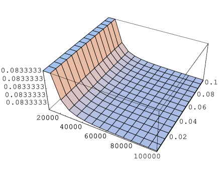
Figure 2: 3D graphic of $\frac{\Delta L}{\dot{M}c^{2}}\times\ell\times M$ where the SMBH mass $M$ varies from 10 to 10⁶ $M_{\odot}$ and the radius $\ell$ of the AdS₅ bulk varies from $10^{-7}$ to $10^{-1}$ mm.

Figure 3: Graphic of $\displaystyle\frac{\Delta L}{\dot{M}c^{2}}\times\ell$ for $M=M_{\odot}$

Figure 4: Graphic of $\displaystyle\frac{\Delta L}{\dot{M}c^{2}}\times\ell$ for $M=100M_{\odot}$

Figure 5: Graphic of $\displaystyle\frac{\Delta L}{\dot{M}c^{2}}\times\ell$ for $M=10^{4}M_{\odot}$

III.2 Corrections in the radius of Kerr SMBHs by brane effects

We now proceed by considering a Kerr BH on the 3-brane. The Kerr metric describing the neighborhood of a spherical rotating BH with mass $M$ and angular momentum $J$, is given by

$$g_{\mu\nu}^{\rm Kerr}=\begin{pmatrix}\omega^{2}\beta^{2}-\alpha^{2}&0&0&-\omega\beta^{2}\\ 0&\frac{\rho^{2}}{\Delta}&0&0\\ 0&0&\rho^{2}&0\\ -\omega\beta^{2}&0&0&\beta^{2}\end{pmatrix}$$ (29)

where

$$\Delta = r^{2}+\frac{a^{2}}{c^{2}}-2\frac{GM}{c^{2}}r,\quad\rho^{2}=r^{2}+\frac{a^{2}}{c^{2}}\cos^{2}\theta,$$ (30)

$$\Sigma^{2} = \left(r^{2}+\frac{a^{2}}{c^{2}}\right)^{2}-\frac{a^{2}}{c^{2}}\Delta\sin^{2}\theta,\quad\beta=\frac{\Sigma}{\rho}\sin\theta,$$

$$\omega = \frac{2aGMr}{c^{3}\Sigma^{2}},\quad\alpha=\left(1-\frac{2GM}{c^{2}r}\right)^{1/2}.$$ (31)

The rotation parameter $a$ is defined by $a=\frac{J}{Mc}$. In order to write the Kerr metric in a diagonal form, if we solve the characteristic eigenvalue equation associated with eq.(29) the eigenvalues are given by

$$\lambda_{2} = \frac{\rho^{2}}{\Delta},\qquad\;\lambda_{3}=\rho^{2},$$

$$\lambda_{1,4} = \frac{1}{2}[(\beta^{2}+\omega^{2}\beta^{2}-\alpha^{2})$$

$$\pm \left((\beta^{2}+\omega^{2}\beta^{2}-\alpha^{2})^{2}-4((\beta^{2}+\omega^{2}\beta^{2})^{2}+\omega\beta^{2})\right)^{1/2}]$$

Now we must impose a condition, that arises when the eigenvalue characteristic equation is solved and we impose the condition for real eigenvalues, i.e.,

$$(1-\omega^{2})^{2}\beta^{4}-4\omega^{2}\beta^{2}+\alpha^{2}[4+\alpha^{2}-2\beta^{2}(1+\omega^{2})]\geq 0$$ (32)

from which the Kerr metric is given in a diagonal form:

$$g^{\rm Kerr} = g_{\mu\nu}^{\rm Kerr}dx^{\mu}dx^{\nu}$$ (33)

$$= \lambda_{1}{dt^{\prime}}^{2}+\frac{dr^{2}}{\frac{\rho^{2}}{\Delta}}+\rho^{2}d\theta^{2}+\lambda^{4}d{\phi^{\prime}}^{2}$$

Here $d\phi^{\prime}$ and $dt^{\prime}$ are 1-form fields on the 3-brane related to $dt$ and d$\phi$ by the new eigenvectors in the associated directions defined by the eigenvalue equation of eq.(29).

The standard internal and external Kerr radii $r_{\pm}$ are obtained by imposing the coefficient ${\frac{\rho^{2}}{\Delta}}$ of $dr^{2}$ in eq.(33) equals zero, i.e.,

$$R_{\pm\rm Kerr}=\frac{GM}{c^{2}}\pm\left(\frac{G^{2}M^{2}}{c^{4}}-\frac{a^{2}}{c^{2}}\right)^{1/2},$$ (34)

and for instance, for a SMBH with mass $M=10^{9}M_{\odot}$, it follows that

$$R_{+\rm Kerr} = 2.76586432072049\times 10^{12}\,{\rm m},$$

$$R_{-\rm Kerr} = 1.98580123723954\times 10^{11}\,{\rm m}.$$ (35)

when $a=0.5\frac{GM}{c}$. When $a=0$, corresponding to the Schwarzschild limit (static BH) case, it follows that $r_{+}=R_{S}=2.96444444444\times 10^{12}$ m.

In order to obtain the correction of the Kerr radii, given by eq.(34), by brane-world effects, we follow the idea presented in eq.(9). We need to find a correction that presents rotational effects, since the frame dragging associated with rotation of Kerr BHs also produces deviations in the above-mentioned perturbation $\psi$, related to the Schwarzschild form in eq.(9). In Kerr BHs, horizon generators are null geodesics that travel around the horizon with angular velocity $\Omega_{H}$, motivating the assumption that the horizon itself has the rotational angular velocity $\Omega_{H}$. Thus, in order to incorporate rotational effects in eq.(11), we define $\xi(r)$ as the deviation from the Kerr form for ${\frac{\rho^{2}}{\Delta}}$ (the term in the denominator of $dr^{2}$ in eq.(33)), and, as a first trial, we suppose the ansatz

$$\xi(r)=-\frac{4GM\ell^{2}}{3r(c^{2}r^{2}+a^{2})}$$ (36)

in such a way that in a static limit ($a\rightarrow 0$), the correction in the gravitational potential satisfies eq.(2), and equivalently eq.(11). We can prove that, at least up to rational functions with denominator polynomial of order $r^{9}$ and respective numerator polynomial of order $r^{6}$, this ansatz is the one that best fits the limit $a\rightarrow 0$ convergence, as we explicitly show in Appendix, although all the twenty six ansatzen we investigate and analyze in Appendix give an error of at most 34%, if compared with the ansatz given by eq.(36). As we want to investigate the order of magnitude concerning the physical effects (as the measurability of quasar luminosity), and not the exact values, all the twenty six ansatzen show the same order of magnitude associated with the variation of luminosity $\Delta L$ , for each fixed value of the rotation parameter $a$. The more complete the ansatz is, the more notorious the extra dimension brane-world effects are shown to be.

It can be shown that analytical functions that are not rational, describing perturbation in the Kerr form as eq.(36), do not necessarily lead Kerr coordinates to Eddington-Finkelstein coordinates in a smooth limit in its derivatives, in the limit when $a\rightarrow 0$. That is precisely the reason why we illustrate in Appendix the amount of rational functions corresponding to their respective ansatzen. Indeed, it is easy to verify that when $a\rightarrow 0$ (Kerr spacetime becomes Schwarzschild), the Kerr coordinates become those of Eddington and Finkelstein, and the Kerr line element becomes the Eddington-Finkelstein one.

Now, the corrections ${R_{\rm Kerrbrane}}$ in the Kerr radii, by brane-world effects, are obtained via the deviated Kerr form, as

$$\frac{\rho^{2}}{\Delta}+\xi(R_{\rm Kerrbrane})=0.$$ (37)

By expanding the expression above and using eqs.(30) and (36) we obtain

$$3c^{2}R_{\rm Kerrbrane}^{5}-6GMR_{\rm Kerrbrane}^{4}+6a^{2}R_{\rm Kerrbrane}^{3}$$

$$-GM\left(6\frac{a^{2}}{c^{2}}+4\ell^{2}\right)R_{\rm Kerrbrane}^{2}+\frac{3a^{4}}{c^{2}}R_{\rm Kerrbrane}$$

$$-4GM\ell^{2}\frac{a^{2}}{c^{2}}\cos^{2}\theta=0.$$ (38)

Using the standard values of $G$ and $c$ in the SI, and adopting again $\ell\approx 0.1$ mm and $M\sim 2\times 10^{39}$ Kg related to a Kerr SMBH, first of all the above expression has five solutions, two of which are complex conjugated each other and another one refers to the singularity given by ${R_{\rm Kerrbrane}}\rightarrow 0$. The other two solutions correspond to the (internal and external) Kerr horizons corrected by brane effects. Eq.(III.2) has no dependence in the azimuthal angle $\theta$, numerically at least up to 17-digit precision. The solutions of eq.(III.2), for various values of $a$, and the relative correction $1-\displaystyle\frac{R_{+\rm Kerr}}{R_{+\rm Kerrbrane}}$ in the external Kerr radius by brane effects, and consequently the variation in the quasar luminosity emission, from eqs.(13) and (14) is given by

$$\Delta L = \frac{GM}{6c^{2}}\left(R_{+{\rm Kerrbrane}}^{-1}-R_{+\rm Kerr}^{-1}\right)\dot{M}c^{2}$$ (39)

$$= \frac{GM}{6c^{2}R_{+\rm Kerr}}\left(\frac{R_{+\rm Kerr}}{R_{+\rm Kerrbrane}}-1\right)\dot{M}c^{2}.$$

Here $R_{+\rm Kerrbrane}$ and $R_{-\rm Kerrbrane}$ denote respectively external and internal Kerr radii, corrected by brane-world extra-dimensional effects. The results in the range $0\leq a\leq\frac{GM}{c}$ are presented in what follows:

$\displaystyle\frac{ac}{GM}$	$1-\displaystyle\frac{R_{+\rm Kerr}}{R_{+\rm Kerrbrane}}$	$\Delta L$ (erg s-1)
$10^{-10}$	$\sim 10^{-7}$	$\sim 10^{28}$
0.1	-0.00501	-7.89489 $\times 10^{31}$
0.2	-0.02021	-3.18278 $\times 10^{32}$
0.3	-0.04611	-7.26195 $\times 10^{32}$
0.4	-0.08375	-1.31914 $\times 10^{33}$
0.5	-0.13505	-2.12705 $\times 10^{33}$
0.6	-0.20344	-3.20417 $\times 10^{33}$
0.7	-0.29549	-4.65397$\times 10^{33}$
0.8	-0.42539	-6.69998$\times 10^{33}$
0.9	-0.63339	-9.97583 $\times 10^{33}$
0.95	-0.81315	-1.28072 $\times 10^{34}$
0.99	-1.10957	-1.74757 $\times 10^{34}$
0.999	-1.31022	-2.06359 $\times 10^{34}$
0.9999	-1.38048	-2.17425 $\times 10^{34}$
0.999999	-1.41080	-2.22202 $\times 10^{34}$

Table 1: Relative correction of Kerr radius concerning brane effects. $R_{+\rm Kerrbrane}$ denotes the external brane-corrected Kerr radius.

The first line in Table 1 attests the validity of the ansatz given by eq.(36), since for the limit $a\rightarrow 0$, the Kerr radius correction by brane effects tends to the Schwarzschild radius correction, given by eq.(23). Clearly, concerning the first line of Table 1, the second column indeed corresponds to eq.(23), while the third column is related to eq.(27).

Figure 6: Graphic of $\left(1-\displaystyle\frac{R_{+\rm Kerr}}{R_{+\rm Kerrbrane}}\right)\times\displaystyle\frac{ac}{GM}$ for a SMBH.

SMBH quasar luminosity variation $\Delta L$ is given in the interval $1.27\times 10^{-2}L_{\odot}\leq\Delta L\leq 3.4237L_{\odot}$, which gives for rotating (Kerr) BHs an observable correction concerning the variation in their associated quasar luminosity. Note that $\Delta L$ is related to the external brane-corrected Kerr radius, and such corrections in $\Delta L$ are negative ones, in the sense that brane effects decrease quasar observed luminosity. If we compare the results with Schwarzschild relative $\Delta L$, the rotation of Kerr BHs are responsible for the increment of 2 up to 5 orders of magnitude in $\Delta L$.

The results shown in Table 1 can be summarized in the graphics in Figs. (7) and (8).

Figure 7: Graphic of ${\Delta L}\times\displaystyle\frac{ac}{GM}$ for $M=10^{9}M_{\odot}$, in the range $0\leq\displaystyle\frac{ac}{GM}\leq 1$.

Figure 8: Graphic of ${\Delta L}\times\displaystyle\frac{ac}{GM}$ for $M=10^{9}M_{\odot}$, in the range $0\leq\displaystyle\frac{ac}{GM}\leq 0.01$.

IV Concluding Remarks and Outlooks

In the present model the variation of quasar luminosity is regarded as an extra-dimensional brane-world effect, and can be immediately estimated by eq.(28), involving the Schwarzschild radius calculated in a brane-world scenario, and the standard Schwarzschild radius of a BH in spacetime. We also investigated the more notorious brane effects regarding rotating, Kerr, BHs that present a variation in their associated quasar luminosity of the order from $0.013$ up to $\approx 5$ solar luminosities, given by eq.(39), also including, besides the ansatz in eq.(36) the other ones given in Appendix. These effects can be conspicuously observed, but it is hard to observe variation in the luminosity of Schwarzschild BHs, which we have shown they are of order $10^{-5}L_{\odot}$. Although Kerr BHs have also been investigated in the light of a brane-world scenario stoj1 ; stoj2 , the correction in the Kerr internal and external radii and its consequent applications in the observability and measurability of the variation in quasar luminosity is completely original, up to our knowledge. For more details on rotating black holes in brane-world scenarios with large extra dimensions see also s1 ; s2 . As we show in Appendix, there are other possible ansatzen that gives SMBH quasar luminosity variation $\Delta L$ in the interval $1.26\times 10^{-2}L_{\odot}\leq\Delta L\leq 4.3868L_{\odot}$, which points, for rotating (Kerr) BHs, an observable correction concerning the variation in their associated quasar luminosity, due, in particular, to the frame dragging.

Considering the fact that real quasars contain high angular momentum rotating BHs, these results lead to an interesting viewpoint: the luminosity observed from distant quasars are produced by bigger BHs than that expected by nowadays previsions. An easy manner to see this is supposing that, by observations, the luminosity of a quasar is estimated to be $L$. Classically, a spinning black hole will produce the luminosity $L+\Delta L$ and the corrected black hole will produce an $L$ luminosity. If we can measure the radius of this black hole we shall see it is bigger than the classical Kerr BH. This could shed new light in astrophysics, for instance, in estimating the necessary time to a stellar-mass BH to grow until be changed in a SMBH, what naturally enlighten the formation history of galaxies in the early universe (to see related works about the growing time of SMBHs see, e.g., ha1 ; ha2 ; ha3 ). This idea will be developed in a forthcoming paper.

The ansatzen used in Appendix lead to an important fact: for a distant observer, when $r\gg a/c$, the ansatzen in eq.(36) and in Appendix lead to the static case ($\xi(r)\rightarrow\psi(r)$), and the Kerr BH can be viewed as Schwarzschild BH, which is the same for $a\rightarrow 0$. The more complete is the ansatz, the more notorious are the effects of brane-world extra dimension in the variation of luminosity $\Delta L$, related to quasars with Kerr BHs. However, variation in luminosity is caused by introduction of brane-world corrections in the BH boundaries: for a local observer, at the boundaries of the BH, the radius $r$ will have magnitude comparable to $a/c$, and rotational effects will be considerable to cause corrections in the Kerr horizon and consequently in the quasar luminosity.

Here we want to point out it is not our main aim to accurately determine exact values for the variation of luminosity $\Delta L$ in quasars related to a Kerr BH, but we indeed want to emphasize the order of magnitude of the corrections in $\Delta L$. The associated order of magnitude, for each fixed value of the rotation parameter $a$, is always the same, and tends to increase as we put high-order polynomials in the ansatzen. A more complete reasoning is shown in details in Appendix.

It is also desirable to calculate the variation of quasar luminosity in a Reissner-Nordstrøm (RN) geometry generated by a charged, static BH. It shall be done in a sequel paper, using formula, equivalent to eq.(9) but now concerning RN metric rs06 ; rs09 ; Da . Brane models for suitable choice of the extra dimension length and of $\ell$ does predict tracks and/or signatures in LHC Maartens ; lhc . Black holes shall be produced in particle collisions at energies possibly below the Planck scale. ADD brane-worlds ad1 ; ad2 ; ad3 also provides a possibility to observe black hole production signatures in the next-generation colliders and cosmic ray detectors lhc1 . With respect to brane-world scenarios endowed with extra dimensions, they can solve the gauge hierarchy problem ko3 ; ko4 ; ko5 ; ko6 with the string scale at the TeV scale, and the only non-supersymmetric string models that can realize the extra-dimensional scenario, have appeared in ko1 ; ko2 . These four dimensional models are non-supersymmetric, where the $D5$-branes wrap $M^{4}\times T^{4}\times\frac{C}{\mathbb{Z}_{N}}$-chiral fermions get localized as open strings stretching in the intersections between $D5$-branes and provide us with exactly the only known string model realization of the extra-dimensional scenario of ad4 . They use intersecting $D5$-branes dimensional orientifold compactifications of type IIB string theory. They also have two large extra dimensions transverse to the intersecting $D5$-branes and as such one can lower the string scale to the TeV region by keeping the Planck scale large ad4 ; ad2 . Also, it must be pointed out that extra dimensions can be compactified on a curved compact hyperbolic manifold s3 ; s4 which volume grows exponentially with radius. In such model, KK spectrum is different from the flat compactification and, in particular, there are no light graviton modes that are the main problem for cosmology. Furthermore, an exponential hierarchy between the usual Planck scale and the true fundamental scale of physics can emerge with only order unity coefficients while the linear size of the internal space remains small. By their characteristics, these models are exactly in between the RS and ADD models.

In the sequel article we will show that, since mini-BHs possess a Reissner-Nordstrøm-like effective behavior under gravitational potential, they feel a 5$D$ gravity and are more sensitive to extra dimension brane effects, and we shall repeat the procedure of this paper for RN mini-BHs, in order to investigate the observation of mini-BHs in LHC and the hierarchy problem. The considerations regarding rotating ADD and RS mini-BHs s5 are to be investigated in the light of RN BHs.

V Acknowledgements

The authors are grateful to Prof. Roy Maartens for his patience and clearing up expositions concerning branes. We are also grateful to Prof. Christos Kokorelis for bringing into our attention some details concerning the hierarchy problem, string models and $D5$-branes, to Prof. Dejan Stojković for clarifying questions regarding rotating black holes in brane models, and to Dr. Ricardo A. Mosna for his helpful computational advisement. Also, the authors are grateful to JCAP referee for enlightening viewpoints and for the suggestions given in order to improve the quality of this paper. CHCA thanks CNPq for financial support.

VI Appendix

Besides the ansatz given by eq.(36), and its associated Table 1, there are other possible ansatzen, among which we can list below some of them. Indeed, it is possible to try other functions, and their associated results are illustrated in what follows. We present, for each ansatz associated to $\xi(r)$, the results in their respective subsequent tables.

1. $\xi(r)=-\displaystyle\frac{4GM\ell^{2}}{3r(c^{2}r^{2}+car+a^{2})}$

   $\displaystyle\frac{ac}{GM}$	$1-\displaystyle\frac{R_{+\rm Kerr}}{R_{+\rm Kerrbrane}}$	$\Delta L$ (erg s-1)
   $10^{-10}$	$\sim 10^{-7}$	$\sim 10^{28}$
   0.1	-0.006012	-8.13192 $\times 10^{31}$
   0.2	-0.02464	-4.05497 $\times 10^{32}$
   0.3	-0.05109	-8.21089 $\times 10^{32}$
   0.4	-0.09645	-1.50464 $\times 10^{33}$
   0.5	-0.18128	-2.69345 $\times 10^{33}$
   0.6	-0.25451	-4.04981 $\times 10^{33}$
   0.7	-0.33546	-5.07349$\times 10^{33}$
   0.8	-0.46913	-7.13873$\times 10^{33}$
   0.9	-0.69564	-1.18734 $\times 10^{34}$
   0.95	-0.88354	-1.40993 $\times 10^{34}$
   0.99	-1.19511	-1.89631 $\times 10^{34}$
   0.999	-1.38556	-2.23880 $\times 10^{34}$
   0.9999	-1.46110	-2.37453 $\times 10^{34}$
   0.999999	-1.49347	-2.42331 $\times 10^{34}$

2. $\xi(r)=-\displaystyle\frac{4GM\ell^{2}}{3cr^{2}(cr+a)}$

   $\displaystyle\frac{ac}{GM}$	$1-\displaystyle\frac{R_{+\rm Kerr}}{R_{+\rm Kerrbrane}}$	$\Delta L$ (erg s-1)
   $10^{-10}$	$\sim 10^{-7}$	$\sim 10^{28}$
   0.1	-0.00734	-8.87120 $\times 10^{31}$
   0.2	-0.026339	-4.08352 $\times 10^{32}$
   0.3	-0.05086	-8.07331 $\times 10^{32}$
   0.4	-0.10537	-1.46741 $\times 10^{33}$
   0.5	-0.16133	-2.71776 $\times 10^{33}$
   0.6	-0.25613	-4.25609 $\times 10^{33}$
   0.7	-0.34881	-5.18734$\times 10^{33}$
   0.8	-0.43524	-7.04734$\times 10^{33}$
   0.9	-0.69335	-1.06498 $\times 10^{34}$
   0.95	-0.86209	-1.38912 $\times 10^{34}$
   0.99	-1.15977	-1.88530 $\times 10^{34}$
   0.999	-1.36129	-2.24378 $\times 10^{34}$
   0.9999	-1.44376	-2.36108 $\times 10^{34}$
   0.999999	-1.46312	-2.41906 $\times 10^{34}$

3. $\xi(r)=-\displaystyle\frac{4GM\ell^{2}r}{3(c^{2}r^{2}+a^{2})^{2}}$

   $\displaystyle\frac{ac}{GM}$	$1-\displaystyle\frac{R_{+\rm Kerr}}{R_{+\rm Kerrbrane}}$	$\Delta L$ (erg s-1)
   $10^{-10}$	$\sim 10^{-7}$	$\sim 10^{28}$
   0.1	-0.00913	-8.54973 $\times 10^{31}$
   0.2	-0.02956	-4.15322 $\times 10^{32}$
   0.3	-0.05731	-8.64175 $\times 10^{32}$
   0.4	-0.10142	-1.56713 $\times 10^{33}$
   0.5	-0.21965	-2.89342 $\times 10^{33}$
   0.6	-0.29231	-4.28744 $\times 10^{33}$
   0.7	-0.38300	-5.18456$\times 10^{33}$
   0.8	-0.51241	-7.39810$\times 10^{33}$
   0.9	-0.73087	-1.23884 $\times 10^{34}$
   0.95	-0.92635	-1.45102 $\times 10^{34}$
   0.99	-1.27391	-1.97662 $\times 10^{34}$
   0.999	-1.57328	-2.38209 $\times 10^{34}$
   0.9999	-1.61298	-2.63901 $\times 10^{34}$
   0.999999	-1.50139	-2.59463 $\times 10^{34}$

4. $\xi(r)=-\displaystyle\frac{4GM\ell^{2}r}{3(c^{2}r^{2}+a^{2})(c^{2}r^{2}+car+a^{2})}$

   $\displaystyle\frac{ac}{GM}$	$1-\displaystyle\frac{R_{+\rm Kerr}}{R_{+\rm Kerrbrane}}$	$\Delta L$ (erg s-1)
   $10^{-10}$	$\sim 10^{-7}$	$\sim 10^{28}$
   0.1	-0.00967	-8.67821 $\times 10^{31}$
   0.2	-0.03174	-4.21755 $\times 10^{32}$
   0.3	-0.059334	-8.72392 $\times 10^{32}$
   0.4	-0.12890	-1.59335 $\times 10^{33}$
   0.5	-0.24509	-2.94252 $\times 10^{33}$
   0.6	-0.31823	-4.33756 $\times 10^{33}$
   0.7	-0.41002	-5.23908$\times 10^{33}$
   0.8	-0.53771	-7.43905$\times 10^{33}$
   0.9	-0.77346	-1.26771 $\times 10^{34}$
   0.95	-0.95327	-1.49214 $\times 10^{34}$
   0.99	-1.30631	-2.01136 $\times 10^{34}$
   0.999	-1.60455	-2.41774 $\times 10^{34}$
   0.9999	-1.64224	-2.66329 $\times 10^{34}$
   0.999999	-1.54598	-2.64902 $\times 10^{34}$

5. $\xi(r)=-\displaystyle\frac{4GM\ell^{2}(r+\frac{a}{c})}{3r^{2}(c^{2}r^{2}+a^{2})}$

   $\displaystyle\frac{ac}{GM}$	$1-\displaystyle\frac{R_{+\rm Kerr}}{R_{+\rm Kerrbrane}}$	$\Delta L$ (erg s-1)
   $10^{-10}$	$\sim 10^{-7}$	$\sim 10^{28}$
   0.1	-0.00821	-8.64319 $\times 10^{31}$
   0.2	-0.02235	-3.94566 $\times 10^{32}$
   0.3	-0.04862	-7.98111 $\times 10^{32}$
   0.4	-0.09134	-1.41398 $\times 10^{33}$
   0.5	-0.15423	-2.63452 $\times 10^{33}$
   0.6	-0.22957	-3.95534 $\times 10^{33}$
   0.7	-0.30414	-5.00451$\times 10^{33}$
   0.8	-0.43524	-6.97134$\times 10^{33}$
   0.9	-0.66819	-1.02457 $\times 10^{34}$
   0.95	-0.83415	-1.35673 $\times 10^{34}$
   0.99	-1.13776	-1.84235 $\times 10^{34}$
   0.999	-1.33411	-2.17996 $\times 10^{34}$
   0.9999	-1.41389	-2.32723 $\times 10^{34}$
   0.999999	-1.43313	-2.37076 $\times 10^{34}$

6. $\xi(r)=-\displaystyle\frac{4GM\ell^{2}r}{(c^{2}r^{2}+car+a^{2})^{2}}$

   $\displaystyle\frac{ac}{GM}$	$1-\displaystyle\frac{R_{+\rm Kerr}}{R_{+\rm Kerrbrane}}$	$\Delta L$ (erg s-1)
   $10^{-10}$	$\sim 10^{-7}$	$\sim 10^{28}$
   0.1	-0.00842	-8.91420 $\times 10^{31}$
   0.2	-0.02529	-4.02583 $\times 10^{32}$
   0.3	-0.05182	-8.03184 $\times 10^{32}$
   0.4	-0.09372	-1.46297 $\times 10^{33}$
   0.5	-0.15814	-2.68207 $\times 10^{33}$
   0.6	-0.25996	-4.04617 $\times 10^{33}$
   0.7	-0.34845	-5.10553$\times 10^{33}$
   0.8	-0.47972	-7.17852$\times 10^{33}$
   0.9	-0.70341	-1.07640 $\times 10^{34}$
   0.95	-0.89352	-1.42865 $\times 10^{34}$
   0.99	-1.21774	-1.95393 $\times 10^{34}$
   0.999	-1.39224	-2.26408 $\times 10^{34}$
   0.9999	-1.48285	-2.43071 $\times 10^{34}$
   0.999999	-1.52619	-2.66318 $\times 10^{34}$

7. $\xi(r)=-\displaystyle\frac{4GM\ell^{2}(r+\frac{a}{c})}{(c^{2}r^{2}+a^{2})^{2}}$

   $\displaystyle\frac{ac}{GM}$	$1-\displaystyle\frac{R_{+\rm Kerr}}{R_{+\rm Kerrbrane}}$	$\Delta L$ (erg s-1)
   $10^{-10}$	$\sim 10^{-7}$	$\sim 10^{28}$
   0.1	-0.00953	-8.98053 $\times 10^{31}$
   0.2	-0.02741	-4.07342 $\times 10^{32}$
   0.3	-0.05671	-8.09554 $\times 10^{32}$
   0.4	-0.09912	-1.50712 $\times 10^{33}$
   0.5	-0.19623	-2.75923 $\times 10^{33}$
   0.6	-0.30745	-4.23076 $\times 10^{33}$
   0.7	-0.39610	-5.30651$\times 10^{33}$
   0.8	-0.52886	-7.38309$\times 10^{33}$
   0.9	-0.76124	-1.36297 $\times 10^{34}$
   0.95	-0.96100	-1.74522 $\times 10^{34}$
   0.99	-1.29054	-2.29364 $\times 10^{34}$
   0.999	-1.47301	-2.51908 $\times 10^{34}$
   0.9999	-1.56772	-2.76221 $\times 10^{34}$
   0.999999	-1.60182	-2.84310 $\times 10^{34}$

8. $\xi(r)=-\displaystyle\frac{4GM\ell^{2}(r+\frac{a}{c})}{(c^{2}r^{2}+car+a^{2})^{2}}$

   $\displaystyle\frac{ac}{GM}$	$1-\displaystyle\frac{R_{+\rm Kerr}}{R_{+\rm Kerrbrane}}$	$\Delta L$ (erg s-1)
   $10^{-10}$	$\sim 10^{-7}$	$\sim 10^{28}$
   0.1	-0.00908	-8.94376 $\times 10^{31}$
   0.2	-0.02595	-4.05387 $\times 10^{32}$
   0.3	-0.054621	-8.06410 $\times 10^{32}$
   0.4	-0.09741	-1.48326 $\times 10^{33}$
   0.5	-0.18845	-2.72164 $\times 10^{33}$
   0.6	-0.28644	-4.20988 $\times 10^{33}$
   0.7	-0.37232	-5.27359$\times 10^{33}$
   0.8	-0.49871	-7.34237$\times 10^{33}$
   0.9	-0.73420	-1.31489 $\times 10^{34}$
   0.95	-0.92755	-1.70367 $\times 10^{34}$
   0.99	-1.24309	-2.22785 $\times 10^{34}$
   0.999	-1.40463	-2.44762 $\times 10^{34}$
   0.9999	-1.50478	-2.66423 $\times 10^{34}$
   0.999999	-1.53287	-2.68250 $\times 10^{34}$

9. $\xi(r)=-\displaystyle\frac{4GM\ell^{2}(r^{2}+\frac{ar}{c}+\frac{a^{2}}{c^{2}})}{3r^{3}(c^{2}r^{2}+car+a^{2})}$

   $\displaystyle\frac{ac}{GM}$	$1-\displaystyle\frac{R_{+\rm Kerr}}{R_{+\rm Kerrbrane}}$	$\Delta L$ (erg s-1)
   $10^{-10}$	$\sim 10^{-7}$	$\sim 10^{28}$
   0.1	-0.00878	-8.91935 $\times 10^{31}$
   0.2	-0.02415	-3.98723 $\times 10^{32}$
   0.3	-0.05064	-8.01176 $\times 10^{32}$
   0.4	-0.18546	-1.43512 $\times 10^{33}$
   0.5	-0.19754	-2.84356 $\times 10^{33}$
   0.6	-0.239758	-4.01574 $\times 10^{33}$
   0.7	-0.31145	-5.12985$\times 10^{33}$
   0.8	-0.44786	-7.34130$\times 10^{33}$
   0.9	-0.68111	-1.05427 $\times 10^{34}$
   0.95	-0.86921	-1.39712 $\times 10^{34}$
   0.99	-1.25475	-1.96459 $\times 10^{34}$
   0.999	-1.38733	-2.31902 $\times 10^{34}$
   0.9999	-1.45616	-2.42564 $\times 10^{34}$
   0.999999	-1.46692	-2.43704 $\times 10^{34}$

10. $\xi(r)=-\displaystyle\frac{4GM\ell^{2}}{3c^{2}r^{3}}\exp\left(\frac{ac}{GM}\right)$

    $\displaystyle\frac{ac}{GM}$	$1-\displaystyle\frac{R_{+\rm Kerr}}{R_{+\rm Kerrbrane}}$	$\Delta L$ (erg s-1)
    $10^{-10}$	$\sim 10^{-7}$	$\sim 10^{28}$
    0.1	-0.0178	-9.0935 $\times 10^{31}$
    0.2	-0.0295	-4.1017 $\times 10^{32}$
    0.3	-0.0528	-8.1352 $\times 10^{32}$
    0.4	-0.2031	-1.4645 $\times 10^{33}$
    0.5	-0.2165	-2.9081 $\times 10^{33}$
    0.6	-0.2546	-4.1024 $\times 10^{33}$
    0.7	-0.3345	-5.2371$\times 10^{33}$
    0.8	-0.4657	-7.4152$\times 10^{33}$
    0.9	-0.7018	-1.1276 $\times 10^{34}$
    0.95	-0.8901	-1.4464 $\times 10^{34}$
    0.99	-1.2879	-2.0183 $\times 10^{34}$
    0.999	-1.412	-2.4132 $\times 10^{34}$
    0.9999	-1.493	-2.4739 $\times 10^{34}$
    0.999999	-1.502	-2.4916 $\times 10^{34}$

11. $\xi(r)=-\displaystyle\frac{4GM\ell^{2}(r^{3}+\frac{a^{2}r}{c^{2}}+\frac{ar^{2}}{c})}{3r^{4}(c^{2}r^{2}+car+a^{2})}$

    $\displaystyle\frac{ac}{GM}$	$1-\displaystyle\frac{R_{+\rm Kerr}}{R_{+\rm Kerrbrane}}$	$\Delta L$ (erg s-1)
    $10^{-10}$	$\sim 10^{-7}$	$\sim 10^{28}$
    0.1	-0.0095	-8.9876 $\times 10^{31}$
    0.2	-0.0270	-4.1746 $\times 10^{32}$
    0.3	-0.0545	-8.0823 $\times 10^{32}$
    0.4	-0.2098	-1.4734 $\times 10^{33}$
    0.5	-0.2154	-2.9065 $\times 10^{33}$
    0.6	-0.2543	-4.0854 $\times 10^{33}$
    0.7	-0.3390	-5.2108$\times 10^{33}$
    0.8	-0.4654	-7.4832$\times 10^{33}$
    0.9	-0.7179	-1.0924 $\times 10^{34}$
    0.95	-0.8951	-1.4132 $\times 10^{34}$
    0.99	-1.2873	-1.9946 $\times 10^{34}$
    0.999	-1.4190	-2.3397 $\times 10^{34}$
    0.9999	-1.4815	-2.4452 $\times 10^{34}$
    0.999999	-1.5185	-2.5304 $\times 10^{34}$

    Here we want to point out it is not our main aim to accurately determine exact values for the variation of luminosity in quasars related to a Kerr BH, but in this first article, we only want to emphasize the order of magnitude of this correction in $\Delta L$. The associated order of magnitude, for each fixed value of the rotation parameter $a$, is always the same, including other ansatzen, like the rational functions listed below:

    $$\xi(r) = -\displaystyle\frac{4GM\ell^{2}r^{2}}{3(c^{3}r^{3}+a^{3})(c^{2}r^{2}+a^{2})},$$

    $$\xi(r) = -\displaystyle\frac{4GM\ell^{2}r^{2}}{3(c^{3}r^{3}+a^{3})(c^{2}r^{2}+car+a^{2})}$$

    $$\xi(r) = -\displaystyle\frac{4GM\ell^{2}r^{2}}{3(c^{3}r^{3}+c^{2}r^{2}a+a^{3})(c^{2}r^{2}+car+a^{2})},$$

    $$\xi(r) = -\displaystyle\frac{4GM\ell^{2}r^{2}}{3(c^{3}r^{3}+c^{2}ar^{2}+ca^{2}r+a^{3})(c^{2}r^{2}+car+a^{2})}$$

    $$\xi(r) = -\displaystyle\frac{4GM\ell^{2}(r^{2}+\frac{a^{2}}{c^{2}})}{3(c^{3}r^{3}+a^{3})(c^{2}r^{2}+a^{2})},$$

    $$\xi(r) = -\displaystyle\frac{4GM\ell^{2}(r^{2}+\frac{a^{2}}{c^{2}})}{3(c^{3}r^{3}+a^{3})(c^{2}r^{2}+car+a^{2})}$$

    $$\xi(r) = -\displaystyle\frac{4GM\ell^{2}(r^{2}+\frac{a^{2}}{c^{2}})}{3(c^{3}r^{3}+c^{2}r^{2}a+a^{3})(c^{2}r^{2}+car+a^{2})},$$

    $$\xi(r) = -\displaystyle\frac{4GM\ell^{2}(r^{2}+\frac{a^{2}}{c^{2}})}{3(c^{3}r^{3}+c^{2}ar^{2}+ca^{2}r+a^{3})(c^{2}r^{2}+car+a^{2})},$$

    $$\xi(r) = -\displaystyle\frac{4GM\ell^{2}(r^{2}+car+\frac{a^{2}}{c^{2}})}{3(c^{3}r^{3}+c^{2}ar^{2}+ca^{2}r+a^{3})(c^{2}r^{2}+car+a^{2})},$$

    $$\xi(r) = -\displaystyle\frac{4GM\ell^{2}(r^{2}+car+\frac{a^{2}}{c^{2}})}{3(c^{3}r^{3}+c^{2}ar^{2}+a^{3})(c^{2}r^{2}+car+a^{2})},$$

    $$\xi(r) = -\displaystyle\frac{4GM\ell^{2}(r^{2}+car+\frac{a^{2}}{c^{2}})}{3(c^{3}r^{3}+c^{2}ar^{2}+ca^{2}r)(c^{2}r^{2}+car+a^{2})},$$

    $$\xi(r) = -\displaystyle\frac{4GM\ell^{2}(r^{3}+\frac{a}{c}r^{2}+\frac{a^{2}}{c^{2}})}{3(c^{3}r^{3}+c^{2}ar^{2}+ca^{2}r+a^{3})^{2}},$$

    $$\xi(r) = -\displaystyle\frac{4GM\ell^{2}(r^{3}+\frac{a}{c}r^{2}+\frac{a^{2}}{c^{2}})}{3(c^{3}r^{3}+c^{2}ar^{2}+ca^{2}r+a^{3})(c^{3}r^{3}+c^{2}ar^{2}+a^{3})},$$

    $$\xi(r) = -\displaystyle\frac{4GM\ell^{2}(r^{3}+\frac{a}{c}r^{2}+\frac{a^{2}}{c^{2}})}{3(c^{3}r^{3}+c^{2}ar^{2}+ca^{2}r+a^{3})(c^{3}r^{3}+ca^{2}r+a^{3})},$$

    $$\xi(r) = -\displaystyle\frac{4GM\ell^{2}(r^{3}+\frac{a}{c}r^{2}+\frac{a^{2}}{c^{2}})}{3(c^{3}r^{3}+ca^{2}r+a^{3})(c^{3}r^{3}+c^{2}ar^{2}+a^{3})},$$

    for instance.

All those formulæ  for the ansatz related to $\xi(r)$ give a value for $\Delta L$ which is shown to be at most 34% bigger than the original ansatz given by eq.(36). Anyway, the RS brane-world extra-dimensional effects, concerning the variation in quasar luminosity $\Delta L$, are always more significant than the original deviation given by eq.(37), coming from eq.(36).

References

- (1) Green M B, Schwarz J H, and Witten E, Superstring Theory, vols. I & II, Cambridge Univ. Press, Cambridge 1987.
- (2) Dienes K R, String theory and the path to unification: a review of recent developments, Phys. Rep. 287, 447-525 (1997) [hep-th/9602045].
- (3) Kaku M, Strings, Conformal Fields and M-theory, Springer-Verlag, New York 2000.
- (4) Kiritsis E, Introduction to Superstring Theory, Leuven Notes in Math. and Theor. Phys. 9, Leuven Univ. Press, Leuven 1997 [hep-ph/9709062].
- (5) Randall L and Sundrum R, An alternative to compactification, Phys. Rev. Lett. 83, 4690-4693 (1999) [hep-th/9906064].
- (6) Randall L and Sundrum R, A large mass hierarchy from a small extra dimension, Phys. Rev. Lett. 83 (1999) 3370-3373 [hep-ph/9905221].
- (7) Rovelli C, Loop quantum gravity, Living Rev. Rel. 1, 1-34 (1998) [gr-qc/9710008].
- (8) Townsend P K, Brane surgery, Nucl. Phys. B Proc. Suppl., 58, 163-175 (1997) [hep-th/9609217].
- (9) Akama K, Pregeometry in Lecture Notes in Physics, 176, Gauge Theory and Gravitation, Kikkawa K, Nakanishi N, and Nariai H (eds.), Proceedings, Nara 1982 pp. 267-271 Springer-Verlag, Berlin 1983, also available in ‘An early proposal of brane world’ [hep-th/0001113].
- (10) Lykken J and Randall L, The shape of gravity, JHEP 06 (2000) 014 [hep-th/9908076].
- (11) Gregory R, Rubakov V A, and Sibiryakov S M, Brane worlds: the gravity of escaping matter, Class. Quant. Grav. 17, 4437-4449 (2000) [hep-th/0003109].
- (12) Maartens R, Brane-world gravity, Living Rev. Relat. 7, 7 (2004) [gr-qc/0312059].
- (13) Seahra S S, Clarkson C, and Maartens R, Detecting extra dimensions with gravity wave spectroscopy: the black string brane-world, Phys. Rev. Lett. 94 (2005) 121302 [gr-qc/0408032].
- (14) Kanno S and Soda J, Black String Perturbations in RS1 Model, in 4th Australasian Conference on General Relativity and Gravitation, Monash University, Melbourne, January 2004. To appear in the proceedings, in General Relativity and Gravitation.
- (15) Emparan R, Garcia-Bellido J, and Kaloper N, Black hole astrophysics in AdS braneworlds, JHEP 0301 (2003) 079 [hep-th/0212132].
- (16) Shiromizu T, Maeda K, and Sasaki M, The Einstein equations on the 3-brane world, Phys. Rev. D62, 024012 (2000) [gr-qc/9910076].
- (17) Dadhich N, Maartens R, Papadopoulos P, and Rezania V, Black holes on the brane, Phys. Lett. B487, 1-6 (2000) [hep-th/0003061].
- (18) Kanti P and Tamvakis K, Quest for Localized 4-D Black Holes in Brane Worlds, Phys. Rev. D65, 084010 (2002) [hep-th/0110298].
- (19) Casadio R, Fabbri A, and Mazzacurati L, New black holes in the brane-world?, Phys. Rev. D65, 084040 (2002) [gr-qc/0111072].
- (20) Kanti P, Olasagasti I, and Tamvakis K, Quest for Localized 4-D Black Holes in Brane Worlds. II : Removing the bulk singularities, Phys. Rev. D68, 124001 (2003) [hep-th/0307201].
- (21) Shiromizu T and Shibata M, Black holes in the brane world:Time symmetric initial data, Phys. Rev. D62, 127502 (2000) [hep-th/0007203]; Chamblin A, Reall H S, Shinkai H A, and Shiromizu T, Charged brane-World black holes, Phys. Rev. D63, 064015 (2001) [hep-th/0008177].
- (22) Casadio R and Mazzacurati L, Bulk shape of brane-world black holes, Mod. Phys. Lett. A18, 651 (2003) [gr-qc/0205129].
- (23) Germani C and Maartens R, Stars in the braneworld, Phys. Rev. D64 124010 (2001) [hep-th/0107011].
- (24) Deruelle N, Stars on branes: the view from the brane [gr-qc/0111065].
- (25) Visser M and Wiltshire D L, On-brane data for braneworld stars, Phys. Rev. D67, 104004 (2003) [hep-th/0212333].
- (26) Giannakis I and Ren H, Possible extensions of the 4D Schwarzschild horizon in the 5D brane world, Phys. Rev. D63, 125017 (2001) [hep-th/0010183].
- (27) Fujii K, A Modern Introduction to Cardano and Ferrari Formulas in the Algebraic Equations [quant-ph/0311102].
- (28) Coimbra-Araújo C H, da Rocha R and Pedron I T, Anti-de Sitter curvature radius constrained by quasars in brane-world scenarios, Int. J. Mod. Phys. D14, to appear [astro-ph/0505132].
- (29) Font J A and Ibáñez J M, Non-axisymmetric relativistic Bondi-Hoyle accretion on to a Schwarzschild black hole, Monthly Not. Royal Astron. Soc., 298 (3) 835-846 (1998) [astro-ph/9810344].
- (30) Shapiro S L and Teukolski S A, Black holes, white dwarfs, and neutron stars, Wiley-Interscience, New York 1983.
- (31) Frolov V P, Fursaev D V, and Stojkovic D, Interaction of higher-dimensional rotating black holes with branes, Class. Quant. Grav. 21 (2004) 3483-3498 [gr-qc/0403054].
- (32) Frolov V P, Fursaev D V, and Stojkovic D, Rotating black holes in brane worlds, JHEP 0406 (2004) 057 [gr-qc/0403002].
- (33) Frolov V P and Stojkovic D, Quantum radiation from a five-dimensional rotating blach hole, Phys. Rev. D67 084004 (2003).
- (34) Frolov V P and Stojkovic D, Particle and light motion in a space-time of a five-dimensional rotating black hole, Phys. Rev. D68 064011 (2003).
- (35) Haehnelt M G and Rees M J, Formation of nuclei in newly-formed galaxies and the evolution of the quasar population, Monthly Not. Royal Astron. Soc. 263, 168 (1993).
- (36) Haehnelt M G and Kauffmann G, The correlation between black hole mass and bulge velocity dispersion in hierarchical galaxy formation models, Monthly Not. Royal Astron. Soc. 318 L35 (2000).
- (37) Kauffmann G and Haehnelt M G, A unified model for the evolution of galaxies and quasars, Monthly Not. Royal Astron. Soc. 311 576 (2000).
- (38) Cavaglia M, Das S, and Maartens R, Will we observe black holes at LHCs?, Class. Quant. Grav. 20 L205-L212 (2003).
- (39) Arkani-Hamed N, Dimopoulos S, and Dvali G, The hierarchy problem and new dimensions at a millimeter, Phys. Lett. B429, 263-272 (1998) [hep-ph/9803315].
- (40) Arkani-Hamed N, Dimopoulos S, and Dvali G, Phenomenology, Astrophysics and Cosmology of Theories with Sub-Millimeter Dimensions and TeV Scale Quantum Gravity, Phys. Rev. D59 (1999) 086004 [hep-ph/9807344].
- (41) Antoniadis I, Arkani-Hamed N, Dimopoulos S, and Dvali G, New dimensions at a millimeter to a Fermi and superstrings at a TeV, Phys. Lett. B436, 257-263 (1998) [hep-ph/9804398].
- (42) Antoniadis I, A possible new dimension at a few TeV, Phys. Lett. B246, 377-384 (1990).
- (43) Starkman G D, Stojkovic D, and Trodden M, Large extra dimensions and cosmological problems, Phys. Rev. D63 103511 (2001) [hep-th/0012226].
- (44) Starkman G D, Stojkovic D, and Mark Trodden, Homogeneity, flatness and ‘large’ extra dimensions, Phys. Rev. Lett. 87 231303 (2001) [hep-th/0106143].
- (45) Stojkovic D, Distinguishing between the small ADD and RS black holes in accelerators, Phys. Rev. Lett. 94 011603 (2005) [hep-ph/0409124].
- (46) Cavaglia M, Black hole and brane production in TeV gravity: A review, Int. J. Mod. Phys. A18, 1843-1882 (2003) [hep-ph/0210296].
- (47) Kokorelis C, Deformed Intersecting D6-Brane GUTS I, JHEP 0211 (2002) 027 [hep-th/0209202].
- (48) Kokorelis C, GUT Model Hierarchies from Intersecting Branes, JHEP 0208 (2002) 018, [hep-th/0203187]
- (49) Dienes K R, Dudas E, and Gherghetta T, A Calculable Toy Model of the Landscape, Phys. Rev. D72 (2005) 026005, [hep-th/0412185].
- (50) Babu K S, Enkhbat T, and Mukhopadhyaya B, Split Supersymmetry from Anomalous U(1), Nucl. Phys. B720 (2005) 47 [hep-ph/0501079].
- (51) Cremades D, Ibañez L E, and Marchesano F, Standard model at intersecting D5-Branes: lowering the string scale, Nucl. Phys. B643 (2002) 93 [hep-th/0205074].
- (52) Kokorelis C, Exact Standard model Structures from Intersecting D5-branes, Nucl. Phys. B677 (2004) 115, [hep-th/0207234].