Generation of Emissions By Fast Particles In Stochastic Media

1 Introduction

Interaction of charged particles with each other and/or with external fields results in emission of electromagnetic radiation. This article considers the emission arising as fast (nonthermal) particles move through media with random inhomogeneities. The nature of these inhomogeneities might be rather arbitrary. One of the simplest examples of inhomogeneities is a distribution of the microscopic particles (atoms or molecules) in an amorphous substance, so the medium is inhomogeneous at microscopic scales (of the order of the mean distance between particles), perhaps remaining uniform (on average) at macroscopic scales.

More frequently, however, real objects are inhomogeneous on macroscopic scales as well. The irregularities might be related to the interfaces between inhomogeneities, variations of the elemental composition, temperature, density, electric, and magnetic field.

Random inhomogeneities of any of these parameters may strongly affect in various ways the generation of electromagnetic emission. For example, the presence of the density inhomogeneities implies that the dielectric permeability tensor is a random function, as well as the refractive indices of the electromagnetic eigen-modes. As a result, the eigen-modes of the uniform medium are not the same as the eigen-modes of the real inhomogeneous medium. The irregularities of the electric and magnetic fields affect primarily the motion of the fast particle (although the effect of the field fluctuations on the dielectric tensor exists as well).

Below we consider one of many emission processes appearing due to or affecting by small-scale random inhomogeneities, namely, diffusive synchrotron radiation arising as fast particles are scattered by the small-scale random fields. This emission process is of exceptional importance since current models of many astrophysical objects (see, e.g., Jaroshek_etal_2005 ; 2Hohda_2004 and references therein) imply generation of rather strong small-scale magnetic fields. The effect of the inhomogeneities on other emission processes is discussed briefly as well.

2 Statistical Methods in the Theory of Electromagnetic Emission

The trajectories of charged particles and the fields created by them are random functions as the particles move through a random medium. Thus, the use of appropriate statistical methods is required to describe the particle motion and the related fields.

2.1 Spectral Treatment of the Random Fields

For a detailed theory of the random fields we refer to a monograph Toptygin_83 and mention here a few important points only. To be more specific, let us discuss some properties of the random magnetic fields. Assume that total magnetic field is composed of regular and random components $\vec{B}(\vec{r},t)=\vec{B}_{0}(\vec{r},t)+\vec{B}_{st}(\vec{r},t)$, such as $\vec{B}_{0}(\vec{r},t)=\left<\vec{B}(\vec{r},t)\right>$ and $\left<\vec{B}_{st}(\vec{r},t)\right>=0$, where the brackets denote the statistical averaging. Note, that the method of averaging depends on the problem considered.

The statistical properties of the random field might be described with a (infinite) sequence of the multi-point correlation functions, the most important of which is the (two-point) second-order correlation function

$$K_{\alpha\beta}^{(2)}(\vec{R},T,\vec{r},\tau)=\left<B_{st,\alpha}(\vec{r}_{1},t_{1})B_{st,\beta}(\vec{r}_{2},t_{2})\right>,$$ (1)

where $\vec{R}=(\vec{r}_{1}+\vec{r}_{2})/2$, $\vec{r}=\vec{r}_{2}-\vec{r}_{1}$, $T=(t_{1}+t_{2})/2$, and $\tau=t_{2}-t_{1}$.

Since the regular and random fields are statistically independent ($\left<B_{0}B_{st}\right>=B_{0}\left<B_{st}\right>=0$), each of them satisfies the Maxwell equations separately. In particular $\vec{\nabla}\cdot\vec{B}_{st}=0$, so only two of three vector components of the random field are independent.

For statistically uniform random field the Fourier transform of the correlator $K_{\alpha\beta}^{(2)}(\vec{r},\tau)$ over spatial and temporal variables $\vec{r}$ and $\tau$ gives rise to the spectral treatment of the random field

$$K_{\alpha\beta}(\vec{k},\omega)=\int{d\vec{r}d\tau\over(2\pi)^{4}}e^{i(\omega\tau-\vec{kr})}K_{\alpha\beta}^{(2)}(\vec{r},\tau).$$ (2)

For example, for the isotropic turbulence we can easily find

$$K_{\alpha\beta}(\vec{k},\omega)=\frac{1}{2}K(\vec{k})\delta(\omega-\omega(\vec{k}))\left(\delta_{\alpha\beta}-{k_{\alpha}k_{\beta}\over k^{2}}\right),$$ (3)

which, in particular, satisfies the Maxwell equation $\vec{\nabla}\cdot\vec{B}_{st}=0$, since the tensor structure of the correlator is orthogonal to the $\bf k$ vector: $k_{\alpha}K_{\alpha\beta}=0$.

Although the spectral shape of the correlators is not unique and may substantially vary depending on the situation, we will adopt for the purpose of the model a quasi-power-law spectrum of the random measures:

$$K({\bf k})=\frac{A_{\nu}}{(k_{min}^{2}+k^{2})^{\nu/2+1}},\ A_{\nu}={\Gamma(\nu/2+1)k_{min}^{\nu-1}\left<A^{2}\right>\over 3\pi^{3/2}\Gamma(\nu/2-1/2)},$$ (4)

where $\nu$ is the spectral index of the turbulence, and the spectrum $K(\vec{k})$ is normalized to $d^{3}k$:

$$\int_{0}^{k_{max}}K(\vec{k})d^{3}k=\left<A^{2}\right>,\ \hbox{for}\ k_{min}\ll k_{max},\ \nu>1,$$ (5)

where $\left<A^{2}\right>$ is the mean square of the corresponding measure of the random field, e.g., $\left<B_{st}^{2}\right>$, $\left<E_{st}^{2}\right>$, $\left<\Delta N^{2}\right>$ etc.

2.2 Emission by Particle Moving along a Stochastic Trajectory

The intensity of the emission of the eigen-mode $\sigma$

$${\cal E}_{\vec{n},\omega}^{\sigma}=(2\pi)^{6}{\omega^{2}n_{\sigma}(\omega)\over c^{3}}|(\vec{e}_{\sigma}\cdot\vec{j}_{\omega,\vec{k}})|^{2}$$ (6)

depends on the trajectory of the radiating charged particle since the Fourier transform $\vec{j}_{\omega,\vec{k}}$ of the corresponding electric current has the form:

$$\vec{j}_{\omega,\vec{k}}=Q\int_{-\infty}^{\infty}\vec{v}(t)\exp(i\omega t-i\vec{k}\vec{r}(t)){dt\over(2\pi)^{4}},$$ (7)

where $Q$ is the charge of the particle. For the stochastic motion of the particle, we have to substitute (7) into (6) and perform the averaging of the corresponding expression:

$${\cal E}_{\vec{n},\omega}^{\sigma}={Q^{2}\omega^{2}n_{\sigma}(\omega)\over 4\pi^{2}c^{3}}Re\int_{-T}^{T}dt\int_{0}^{\infty}d\tau e^{i\omega\tau}\left<e^{-i\vec{k}[\vec{r}(t+\tau)-\vec{r}(t)]}(\vec{e}^{*}_{\sigma}\cdot\vec{v}(t+\tau))(\vec{e}_{\sigma}\cdot\vec{v}(t))\right>,$$ (8)

where $2T$ is the total time at which the emission occurs, and $\vec{e}_{\sigma}$ is the polarization vector of the eigen-mode $\sigma$.

It is convenient to perform the averaging denoted by the brackets with the use of the distribution function of the particle(s) $F(\vec{r},\vec{p},t)$ at the time $t$ and the conditional probability $W(\vec{r},\vec{p},t;\vec{r}^{\prime},\vec{p}^{\prime},\tau)$ for the particle to transit from the state $(\vec{r},\vec{p})$ to the state $(\vec{r}^{\prime},\vec{p}^{\prime})$ during the time $\tau$. For statistically uniform random field we obtain:

$${\cal E}_{\vec{n},\omega}^{\sigma}={Q^{2}\omega^{2}n_{\sigma}(\omega)\over 4\pi^{2}c^{3}}Re\int_{-T}^{T}dt\int_{0}^{\infty}d\tau e^{i\omega\tau}\int d\vec{r}d\vec{p}d\vec{p}^{\prime}(\vec{e}^{*}_{\sigma}\cdot\vec{v}^{\prime})(\vec{e}_{\sigma}\cdot\vec{v})F(\vec{r},\vec{p},t)W_{\vec{k}}(\vec{p},t;\vec{p}^{\prime},\tau).$$ (9)

Then, the integration over $\tau$ gives rise to the temporal Fourier transform of $W$, so the spectrum of emitted electromagnetic waves is expressed via the spatial and temporal Fourier transform of the distribution function of the particle in the presence of the random field.

2.3 Kinetic Equation in the Presence of Random Fields

The conditional probability $W$, which substitutes the particle trajectory in the presence of random fields, can be obtained from the kinetic Boltzman equation:

$${\partial f\over\partial t}+\vec{v}{\partial f\over\partial\vec{r}}+\vec{F}_{L}{\partial f\over\partial\vec{p}}=0,$$ (10)

where $\vec{F}_{L}=Q\vec{E}+\frac{Q}{c}[\vec{v},\vec{B}]$ is the Lorentz force, while the electric ($\vec{E}$) and magnetic ($\vec{B}$) fields contain in the general case both regular and random components. Let us express the Lorentz force as a sum of these two components explicitly:

$$\vec{F}_{L}=\vec{F}_{R}+\vec{F}_{st}.$$ (11)

Accordingly, we’ll seek a distribution function in the form of the sum of the averaged ($W$) and fluctuating ($\delta W$) components:

$$f(\vec{r},\vec{p},t)=W(\vec{r},\vec{p},t)+\delta W(\vec{r},\vec{p},t).$$ (12)

Equation for the averaged component $W$ can be derived from (10) with the Green function method Toptygin_83 (magnetic fields only are included below for simplicity):

$${\partial W\over\partial t}+\vec{v}{\partial W\over\partial\vec{r}}-(\vec{\Omega}\overrightarrow{{\cal O}})W=\frac{1}{2}\left(\frac{Qc}{{\cal E}}\right)^{2}\int_{-\infty}^{\infty}d\tau{\cal O}_{\alpha}T_{\alpha\beta}(\vec{\Delta r}(\tau),\tau){\cal O}_{\beta}W(\vec{r}-\vec{\Delta r}(\tau),\vec{p}-\vec{\Delta p}(\tau),t-\tau),$$ (13)

where

$$\vec{\Omega}=\frac{Q\vec{B}c}{\cal E}$$ (14)

is the vector directed as the magnetic field, whose magnitude equals the relativistic gyrofrequency of the charged particle with energy ${\cal E}$,

$$T_{\alpha\beta}(\vec{r},\tau)=\left<B_{st,\alpha}(\vec{r}_{1},t_{1})B_{st,\beta}(\vec{r}_{2},t_{2})\right>={\left<B_{st}^{2}\right>\over 3}\left\{\psi(r)\delta_{\alpha\beta}+\psi_{1}(r){r_{\alpha}r_{\beta}\over r^{2}}\right\}.$$ (15)

To derive (13) we transformed the terms with the magnetic field using the following property of the scalar triple product:

$$\frac{Q}{c}[\vec{vB}]\frac{\partial}{\partial\vec{p}}=-\frac{Q\vec{B}}{c}[\vec{v}\frac{\partial}{\partial\vec{p}}]=-\frac{Q\vec{B}c}{\cal E}\vec{{\cal O}},\qquad\vec{{\cal O}}=[\vec{v}\frac{\partial}{\partial\vec{v}}],$$ (16)

where $\vec{{\cal O}}$ is the operator of the velocity angular variation.

Equation (13) is rather general and can be applied to the study of both emission by fast particles and particle propagation in the plasma Toptygin_83 . Further simplifications of equation (13) can be done by taking into account some specific properties of the problems considered. The theory of wave emission involves a fundamental measure called the coherence length (or the formation zone) that refers to that part of the particle path where the elementary radiation pattern is formed.

The coherence length is much larger than the wavelength for the case of relativistic particles, e.g., the coherence length for synchrotron radiation in the presence of the uniform magnetic field is $l_{s}=R_{L}/\gamma=Mc^{2}/(QB)$, where $R_{L}$ is the Larmour radius, $\gamma={\cal E}/Mc^{2}$ is the Lorentz-factor of the particle. Length $l_{s}$ is by the factor of $\gamma^{2}$ larger than the corresponding wave length. The effect of magnetic field inhomogeneity on the elementary radiation pattern is specified by the ratio of the spatial scale of the field inhomogeneity and the coherence length. If the scale of inhomogeneity is much larger than the coherence length, the effect of the inhomogeneity is small and can typically be discarded. However, if the magnetic field changes noticeably at the coherence length, the inhomogeneity affects the emission strongly, so the spectral and angular distributions of the intensity and polarization of the emission can be remarkably different from the case of the uniform field.

This means, in particular, that in the presence of magnetic turbulence with a broad distribution over the spatial scales, the large-scale spatial irregularities should be considered like the regular field, while the small-scale fluctuations should be properly taken into account as the random field. Since the variation of the particle speed (momentum) over the correlation length of the small-scale random field is small, then we can adopt $\Delta\vec{p}(\tau)=0$, $\Delta\vec{r}(\tau)=\vec{v}\tau$ in the right-hand-side of Eq. (13) . Then, the kinetic equation takes the form

$${\partial W\over\partial t}+\vec{v}{\partial W\over\partial\vec{r}}-(\vec{\Omega}\overrightarrow{{\cal O}})W={\left<B_{st}^{2}\right>\over 6}\left(\frac{Qc}{{\cal E}}\right)^{2}{\cal O}^{2}\int_{-\infty}^{\infty}d\tau\psi(v\tau)W(\vec{r}-\vec{v}\tau,\vec{p},t-\tau).$$ (17)

2.4 Solution of the Kinetic Equation

Let us outline the solution of the kinetic equation (17) for the averaged distribution function $W$. First of all, the stochastic field may require splitting onto large-scale ($\widetilde{\vec{B}}$) and small-scale ($\vec{B}_{st}$) components. To see this, consider a purely sinusoidal spatial wave of the magnetic field with the strength $B_{0}$ and the wavelength $\lambda_{0}=2\pi/k_{0}$. If the wavelength $\lambda_{0}$ is less than the coherence length $l_{s0}$ calculated for the emission in uniform field $B_{0}$, $l_{s0}\sim Mc^{2}/(QB_{0})$, this wave represents the small-scale field, whose spatial inhomogeneity is highly important for the emission; in the opposite case, $\lambda_{0}\ \raise 3.0pt\hbox{$>$}\kern-8.5pt\raise-2.0pt\hbox{$\sim$}\ l_{s0}$, it is the large-scale field.

The splitting is less straightforward when the random field is a superposition of the random waves with a quasi-continuous distribution over the spatial scales. Let us consider the effect provided by a random magnetic field corresponding to a small range $\Delta k$ in the spectrum (4) on the charged particle trajectory. The energy of this magnetic field is

$$\delta{\cal E}_{st}\sim K(\vec{k})k^{2}\Delta k,$$ (18)

the corresponding nonrelativistic “gyrofrequency” is $\delta\omega_{st}\sim Q\sqrt{\delta{\cal E}_{st}}/(Mc)$. For a truly random field, when the harmonics with $\vec{k}$ and $\vec{k}+d\vec{k}$ are essentially uncorrelated, we can arbitrarily select the value $\Delta k$ to be small enough to satisfy $\delta\omega_{st}\ll kc$ for any $k$, so all the independent field components represent the small-scale field. However, in a more realistic case the Fourier components of the random field with similar yet distinct $\vec{k}$ are typically correlated, so they disturb the particle motion coherently and $\Delta k$ in estimate (18) cannot be arbitrarily small any longer. Accordingly, all components of the random field with $k\ \raise 3.0pt\hbox{$<$}\kern-8.5pt\raise-2.0pt\hbox{$\sim$}\ \delta\omega_{st}/c$ (where $\delta\omega_{st}$ is calculated for the smallest allowable $\Delta k$) must be treated as the large-scale field.

The large-scale field $\widetilde{\vec{B}}$ together with the regular field $\vec{B}_{0}$ specifies the vector $\vec{\Omega}$ in the left-hand-side of equation (17):

$$\vec{\Omega}=\frac{Q(\vec{B}_{0}+\widetilde{\vec{B}})c}{\cal E}.$$ (19)

For the analysis of the emission process (and, respectively, for the solution of the kinetic equation (17)), we treat the large-scale field (which is the sum of the regular and large-scale stochastic fields in a general case) as uniform, ($\vec{\Omega}=const$); the actual inhomogeneity might be taken into account by averaging the final expressions of the emission if necessary.

Equation (17) in the presence of both uniform and random magnetic fields has been solved in Topt_Fl_1987 (sf Migdal ):

$$W_{\vec{k}}=\frac{1}{p^{2}}\delta(p-p_{0})\exp\left[-i\frac{\omega v}{c}\left(1-\frac{\omega_{pe}^{2}}{2\omega^{2}}\right)\tau\right]w(\vec{\theta}_{0},\vec{\theta},\tau),$$ (20)

where

$$w(\vec{\theta}_{0},\vec{\theta},\tau)=\frac{x}{\pi\sinh z\tau}\exp\left[-x(\theta^{2}+\theta_{0}^{2})\coth z\tau+2x\vec{\theta}\vec{\theta}_{0}\sinh^{-1}z\tau-\frac{(\vec{\theta}-\vec{\theta}_{0})[\vec{n\Omega}]}{2q}-\frac{\Omega_{\bot}^{2}\tau}{4q}\right],$$ (21)

$$\vec{\theta}_{0}=\frac{\vec{v}_{0}}{v}-\vec{n}\left(1-\frac{\theta_{0}^{2}}{2}\right),\qquad\vec{\theta}=\frac{\vec{v}}{v}-\vec{n}\left(1-\frac{\theta^{2}}{2}\right),$$ (22)

$$x=(1-i)\left(\frac{\omega}{16q}\right)^{1/2};\qquad z=(1-i)(\omega q)^{1/2},$$ (23)

$$q(\omega,\theta)=\pi\left(\frac{Qc}{{\cal E}}\right)^{2}\int d\vec{k}^{\prime}K(\vec{k}^{\prime})\delta(\omega-(\vec{k}-\vec{k}^{\prime})\vec{v}).$$ (24)

If there is only random field and no regular field, function $w$ reads

$$w(\vec{\theta}_{0},\vec{\theta},\tau)=\frac{x}{\pi\sinh z\tau}\exp\bigg{\{}-x(\theta^{2}+\theta^{2}_{0})\coth z\tau+2x\vec{\theta}\vec{\theta}_{0}\sinh^{-1}z\tau\bigg{\}},$$ (25)

in the opposite case where there is no random field, we have

$$w(\vec{\theta}_{0},\vec{\theta},\tau)=\delta(\vec{\theta}-\vec{\theta}_{0}+[\vec{n}\vec{\Omega}]\tau)\exp\bigg{\{}\frac{i\omega\tau}{2}\left[\theta_{0}^{2}-\vec{\theta}_{0}[\vec{n}\vec{\Omega}]\tau+\frac{\Omega_{\bot}^{2}\tau^{2}}{3}\right]\bigg{\}}.$$ (26)

Calculation of the emission with the use of this distribution function leads evidently to the standard expressions of synchrotron radiation in the uniform magnetic field.

Finally, the distribution function of the free particle (moving without any acceleration), which does not produce any emission in the vacuum or uniform plasma, is

$$w^{0}(\vec{\theta}_{0},\vec{\theta},\tau)=\delta(\vec{\theta}-\vec{\theta}_{0})\exp\bigg{\{}\frac{i\omega\tau}{2}\theta^{2}\bigg{\}}.$$ (27)

3 Emission by Relativistic Particles in the Presence of Random Magnetic Field

3.1 General Case

Let us consider the energy emitted by a single particle (regardless the polarization) based on general expression (9), i.e., take the sum of (9) over two orthogonal eigen-modes:

$${\cal E}_{\vec{n},\omega}={Q^{2}\omega^{2}\sqrt{\varepsilon(\omega)}\over 2\pi^{2}c^{3}}Re\int_{-T}^{T}dt\int_{0}^{\infty}d\tau e^{i\omega\tau}\int d\vec{r}d\vec{p}d\vec{p}^{\prime}[\vec{n}\vec{v}^{\prime}]\cdot[\vec{n}\vec{v}]F(\vec{r},\vec{p},t)W_{\vec{k}}(\vec{p},t;\vec{p}^{\prime},\tau),$$ (28)

where we neglected the difference between the two refractive indices in the magnetized plasma and adopted $n_{\sigma}(\omega)\approx\sqrt{\varepsilon(\omega)}$.

In the presence of statistically uniform and stationary magnetic field the emitted energy (28) is proportional to the time (on average), although the intensity of emission at a given direction $\vec{n}$ depends on time since the angle between the instantaneous particle velocity $\vec{v}(t)$ and $\vec{n}$ changes with time as described by the dependence of the function $F(\vec{r},\vec{p},t)$ on time $t$. This kind of the temporal dependence is not of particular interest, e.g., it represents periodic pulses provided by the rotation of the particle in the uniform magnetic field, so it is more convenient to proceed with time-independent intensity of radiation emitted into the full solid angle

$$I_{\omega}=\frac{Q^{2}\omega^{2}}{2\pi^{2}c}\sqrt{\varepsilon(\omega)}Re\int_{0}^{\infty}d\tau\exp\left[\frac{i\omega\tau}{2\gamma^{2}}\left(1+\frac{\omega_{pe}^{2}\gamma^{2}}{\omega^{2}}\right)\right]\int d^{2}\theta d^{2}\theta^{\prime}({\vec{\theta}}{\vec{\theta}^{\prime}})(w({\vec{\theta}},{\vec{\theta}^{\prime}},\tau)-w^{0}({\vec{\theta}},{\vec{\theta}^{\prime}},\tau)),$$ (29)

where $w^{0}({\vec{\theta}},{\vec{\theta}^{\prime}},\tau)$ – the distribution function of the free particle (27), which does not contribute to the electromagnetic emission (since the Vavilov-Cherenkov condition cannot be fulfilled in the plasma or vacuum). Then, calculation of (29), described in detail in Topt_Fl_1987 and reformulated here to more convenient notations, results in

$$I_{\omega}=\frac{8Q^{2}q(\omega)}{3\pi c}\gamma^{2}\left(1+\frac{\omega_{pe}^{2}\gamma^{2}}{\omega^{2}}\right)^{-1}\Phi_{1}(s,r)+\frac{Q^{2}\omega}{4\pi c\gamma^{2}}\left(1+\frac{\omega_{pe}^{2}\gamma^{2}}{\omega^{2}}\right)\Phi_{2}(s,r),$$ (30)

where $\Phi_{1}(s,r)$ and $\Phi_{2}(s,r)$ stand for the integrals:

$$\Phi_{1}(s,r)=24s^{2}Im\int_{0}^{\infty}dt\exp(-2s_{0}t)\left[\coth t\exp\left(-2rs_{0}^{3}(\coth t-\sinh^{-1}t-t/2)\right)-\frac{1}{t}\right],$$ (31)

$$\Phi_{2}(s,r)=4rs^{2}Re\int_{0}^{\infty}dt\frac{\cosh t-1}{\sinh t}\exp\left(-2s_{0}t-2rs_{0}^{3}(\coth t-\sinh^{-1}t-t/2)\right),$$ (32)

which depend on the dimensionless parameters $s_{0}$, $s$, $r$:

$$s_{0}=(1-i)s=\frac{1-i}{8\gamma^{2}}\left(\frac{\omega}{q(\omega)}\right)^{1/2}\left(1+\frac{\omega_{pe}^{2}\gamma^{2}}{\omega^{2}}\right),$$ (33)

$$r=32\gamma^{6}\left(\frac{\Omega_{\bot}}{\omega}\right)^{2}\left(1+\frac{\omega_{pe}^{2}\gamma^{2}}{\omega^{2}}\right)^{-3}.$$ (34)

The parameter $s$ depends on the rate of scattering of the particle by magnetic inhomogeneities $q(\omega)$, which has the form

$$q(\omega)=\frac{\sqrt{\pi}\Gamma(\nu/2)\omega_{st}^{2}\omega_{0}^{\nu-1}}{3\Gamma(\nu/2-1/2)\gamma^{2}(\alpha^{2}+\omega_{0}^{2})^{\nu/2}},$$ (35)

for power-law distribution (4) of magnetic irregularities over scales: $P(k)=4\pi K(\vec{k})k^{2}\propto k^{-\nu}$ at $k\gg k_{min}=\omega_{0}/c$, where $\omega_{st}^{2}=Q^{2}\left<B_{st}^{2}\right>/(Mc)^{2}$ is the square of the cyclotron frequency in the random magnetic field, $\alpha=(a\omega/2)\left(\gamma^{-2}+\omega_{pe}^{2}/\omega^{2}\right)$, $a$ is a factor of the order of unity.

Integrals (31, 32) cannot be expressed with elementary functions in the general case. However, there are convenient asymptotic expressions of these integrals. In particular, if $r\gg 1$ and $rs^{3}\gg 1$ we have

$$\Phi_{1}\approx-8\pi s^{2},\qquad\Phi_{2}\approx 2^{1/3}3^{1/6}\Gamma(2/3)r^{1/3},$$ (36)

while for $s\gg 1$, $r\ll 1$, functions $\Phi_{1}$ and $\Phi_{2}$ contain exponentially small terms:

$$\Phi_{1}\approx 1-3\pi^{1/2}2^{3/4}r^{1/4}s^{2}\exp\left(-\frac{8\sqrt{2}}{3\sqrt{r}}\right),\qquad\Phi_{2}\approx\frac{r}{64s^{2}}+2^{3/4}\pi^{1/2}r^{1/4}\exp\left(-\frac{8\sqrt{2}}{3\sqrt{r}}\right).$$ (37)

Complementary, for $s\ll 1$ and $rs^{3}\ll 1$ we obtain:

$$\Phi_{1}\approx 6s\frac{1-rs^{2}}{1+r^{2}s^{4}},\qquad\Phi_{2}\approx\frac{rs}{2}\frac{1+rs^{2}}{1+r^{2}s^{4}}.$$ (38)

3.2 Special cases

The radiation intensity (30) depends on many parameters, allowing many different parameter regimes. It is clear that in the absence of the random fields we obtain standard synchrotron radiation in a uniform magnetic field. Let us consider here a few interesting cases when the presence of small-scale random field results in a considerable change of the emission.

Weak Random Magnetic Inhomogeneities Superimposed on Regular Magnetic Field

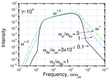
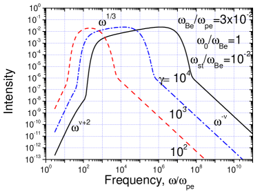
Figure 1: Spectra of radiation by a relativistic particle with $\gamma=10^{4}$ for differing value of the random magnetic field (left) and with different $\gamma$ in the presence of weak random magnetic field $\left<B_{st}^{2}\right>/B_{0}^{2}=10^{-4}$ (right).

Consider the case of weak magnetic irregularities with a broad (power-law) distribution over spacial scales, $B_{\bot}^{2}\gg\left<\widetilde{B}^{2}\right>$, so that

$$\omega_{B}\gg\widetilde{\omega}_{st}\gg\omega_{0},$$ (39)

here $\widetilde{\omega}_{st}$ is the gyro-frequency related to the total random field $\left<\widetilde{B}^{2}\right>^{1/2}$.

Radiation by highly relativistic particles Topt_Fl_1987 is mainly specified by the large-scale (regular plus random) field, since either $s\gg 1$ or $rs^{3}\gg 1$. However, at high frequencies, where synchrotron radiation decreases exponentially, the spectrum is controlled by the small-scale field: the spectral index of radiation is equal to the spectral index of the random field, see fig. 1.

However, a more interesting regime, which has not been considered so far, takes place for moderately relativistic (and possibly non-relativistic) particles moving in a dense plasma (the case typical for solar and geospace plasmas), when synchrotron radiation is known to be exponentially suppressed according to (37) by the effect of plasma density (Razin-effect Razin ; Ginzburg_Syrovatsky_1965 ) at all frequencies. The contribution of the small-scale random field, which we refer to as diffusive synchrotron radiation, in this conditions takes the form:

$$I_{\omega}=\frac{2^{\nu+1}\Gamma(\nu/2)(\nu^{2}+7\nu+8)}{3\sqrt{\pi}\Gamma(\nu/2-1/2)(\nu+2)^{2}(\nu+3)}\ \frac{Q^{2}}{c}\ \frac{\omega_{st}^{2}\omega_{0}^{\nu-1}\gamma^{2\nu}}{\omega^{\nu}\left(1+\frac{\omega_{pe}^{2}\gamma^{2}}{\omega^{2}}\right)^{\nu+1}}.$$ (40)

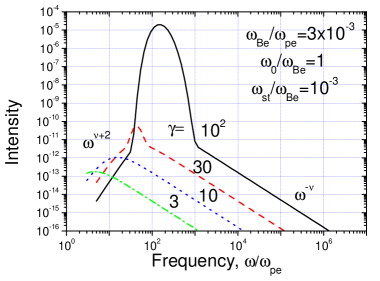
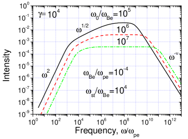
Figure 2: Spectra of radiation by a relativistic particle with different $\gamma$ in a dense plasma in the presence of weak random magnetic field $\left<B_{st}^{2}\right>/B_{0}^{2}=10^{-6}$ (left), and with $\gamma=10^{4}$ in small-scale random magnetic field (right). If $\omega_{0}$ is big enough (e.g., $\omega_{0}/\omega_{Be}=10^{7}$ in the figure) the spectral region provided by multiple scattering, $\omega^{1/2}$, disappears.

It is important that this radiation decreases with the increase of the plasma density (plasma frequency) much more slowly (as a power-law, $\sim\omega_{pe}^{-\nu}$) than synchrotron radiation. As a result, the diffusive synchrotron radiation can dominate the entire spectrum even if the random field is much weaker than the regular field, as is evident from fig. 2 left: the emission by particles with $\gamma\ \raise 3.0pt\hbox{$<$}\kern-8.5pt\raise-2.0pt\hbox{$\sim$}\ 10$ is defined exclusively by the small-scale field.

Small-Scale Magnetic field

Consider an extreme case, which is probably relevant for the physics of cosmological gamma-ray bursts, when there is only small-scale random magnetic field but no (very weak) regular field, so that $\omega_{0}\gg\omega_{st}$ Fleishman_ph_2005 . Now, the parameter $q$ depends substantially on $\omega_{0}$, the particle motion is similar to the random walk, so the radiation spectrum is similar to some extent to bremsstrahlung provided by multiple scattering of the fast particle by randomly located Coulomb centers. In particular, the spectrum of diffusive synchrotron radiation can contain a flat region (as standard bremsstrahlung) and $\propto\omega^{1/2}$ region (like bremsstrahlung suppressed by multiple scattering), fig. 2 right. However, at sufficiently high frequencies ($\omega>\omega_{0}\gamma^{2}$), the flat spectrum gives way to a power-law region $\propto\omega^{-\nu}$ typical for the diffusive synchrotron radiation. We should note, that the spectrum depends significantly on the energy of radiating particle, fig. 3 left, for low-energy particles some parts of the spectrum (e.g., flat region) might be missing.

3.3 Emission by an Ensemble of Particles

The results presented in the previous section can be directly applied for mono-energetic electron distributions, which can be obtained in the laboratory, but are rare exception in nature (e.g., astro- and geo- plasmas). Natural particle distributions can frequently be approximated by a power-law, say, as a function of dimensionless parameter $\gamma$:

$$dN_{e}(\gamma)=(\xi-1)N_{e}\gamma_{1}^{\xi-1}\gamma^{-\xi},\ \ \gamma_{1}\leq\gamma\leq\gamma_{2},$$ (41)

where $N_{e}$ is the number density of relativistic electrons with energies ${\cal E}\geq mc^{2}\gamma_{1}$, $\xi$ is the power-law index of the distribution. Evidently, the intensity of incoherent radiation produced by ensemble (41) of electrons from the unit source volume is

$$P_{\omega}=\int I_{\omega}dN_{e}(\gamma).$$ (42)

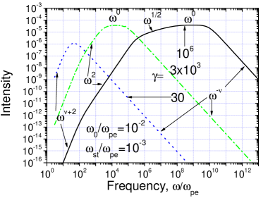
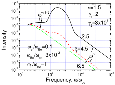
Figure 3: Spectra of radiation by a relativistic particle with different $\gamma=30,~{}3\cdot 10^{3},~{}10^{6}$ in the presence of small-scale random magnetic field (left). Emissivity by fast electron ensemble with different energetic spectra ($\xi=2.5,~{}4.5,~{}6.5$) for the case of dense plasma, $\omega_{Be}/\omega_{pe}=3\cdot 10^{-3}$ (right).

Hard Electron Spectrum.

As we will see, the radiation spectrum produced by an ensemble of particles differs for hard ($\xi<2\nu+1$) and soft ($\xi>2\nu+1$) distributions of fast electrons over energy. Let us consider first the case of hard spectrum Topt_Fl_1987 , which is typical, e.g., for supernova remnants and radio galaxies. Assuming the small-scale field to be small compared with the regular field, we may expect the contribution of diffusive synchrotron radiation to be noticeable only in those frequency ranges where synchrotron emission is small.

In particular, at low frequencies $\omega\ll\max(\omega_{pe}^{2}/\omega_{B\bot},\omega_{pe}\sqrt{\omega_{pe}\gamma_{1}/\omega_{B\bot}})$, synchrotron radiation is suppressed by the effect of density. Diffusive synchrotron radiation is produced by relatively low energy electrons at these frequencies, each electron produces the emission according to (40), which peaks at $\omega\sim\omega_{pe}\gamma$. Evaluation of the integral (42) gives rise to

$$P_{\omega}\simeq\frac{(\xi-1)\Gamma(\nu/2)(\nu^{2}+7\nu+8)}{3\sqrt{\pi}\Gamma(\nu/2-1/2)(\nu+2)^{2}(\nu+3)}\ \frac{e^{2}N_{e}\gamma_{1}^{\xi-1}}{c}\ \frac{\omega_{st}^{2}\omega_{0}^{\nu-1}}{\omega_{pe}^{\nu}}\left(\frac{\omega}{\omega_{pe}}\right)^{\nu+1-\xi}$$ (43)

in agreement with Nik_Tsyt_1979 . This spectrum can either increase or decrease with frequency depending on spectral indices $\nu$ and $\xi$. This expression holds at the frequencies $\omega\gg\omega_{pe}\gamma_{1}$. If there are no particles with $\gamma<\gamma_{1}$, the spectrum at even lower frequencies drops as $P_{\omega}\propto\omega^{\nu+2}$:

$$P_{\omega}=\frac{(\xi-1)2^{\nu+1}\Gamma(\nu/2)(\nu^{2}+7\nu+8)}{3(\xi+1)\sqrt{\pi}\Gamma(\nu/2-1/2)(\nu+2)^{2}(\nu+3)}\ \frac{e^{2}N_{e}}{c}\ \frac{\omega_{st}^{2}\omega_{0}^{\nu-1}\omega^{\nu+2}}{\gamma_{1}^{2}\omega_{pe}^{2\nu+2}}.$$ (44)

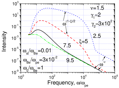
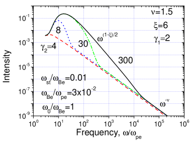
Figure 4: Left: Same as in fig. 3, right, for less dense plasma, $\omega_{Be}/\omega_{pe}=3\cdot 10^{-2}$. The contribution from the uniform field (synchrotron radiation) decreases for softer electron spectra (i.e., as $\xi$ increases). Right: Emissivity by fast electron ensemble (with $\xi=6$) from dense plasma ($\omega_{Be}/\omega_{pe}=3\cdot 10^{-2}$) in the presence of weak magnetic inhomogeneities $\left<B_{st}^{2}\right>/B_{0}^{2}=10^{-4}$ for different high-energy cut-off values $\gamma_{2}$. When $\gamma_{2}$ is small enough, the uniform magnetic field does not affect the radiation spectrum.

At high frequencies $\max(\omega_{pe}^{2}/\omega_{B\bot},\omega_{pe}\sqrt{\omega_{pe}\gamma_{1}/\omega_{B\bot}})\ll\omega\ll\omega_{B\bot}\gamma_{2}^{2}$, where the effect of density is not important, the spectrum is specified by standard synchrotron radiation. However, at higher frequencies, $\omega\gg\omega_{B\bot}\gamma_{2}^{2}$ the intensity of synchrotron radiation decreases exponentially, and the diffusive synchrotron radiation dominates again. Adding up contributions from all particles described by (40) at these frequencies, we obtain

$$P_{\omega}=\frac{2^{\nu+1}(\xi-1)\Gamma(\nu/2)(\nu^{2}+7\nu+8)}{3\sqrt{\pi}(2\nu-\xi+1)\Gamma(\nu/2-1/2)(\nu+2)^{2}(\nu+3)}\ \frac{e^{2}N_{e}\gamma_{1}^{\xi-1}}{c}\ \frac{\omega_{st}^{2}\omega_{0}^{\nu-1}\gamma_{2}^{2\nu-\xi+1}}{\omega^{\nu}}.$$ (45)

Thus, power-law spectrum of relativistic electrons with a cut-off at the energy ${\cal E}=mc^{2}\gamma_{2}$ produce diffusive synchrotron radiation at high frequencies, whose spectrum shape is defined by the small-scale field spectrum. Remarkably, the corresponding flattening in the synchrotron cut-off region has recently been detected in the optical-UV range for the 3C273 jet 3C273_jet , which would imply the presence of relatively strong small-scale field there in agreement with the model 2Hohda_2004 .

Although formally spectrum (45) is valid at arbitrarily high frequencies, there is actually a cut-off related to the minimal scale of the random field $l_{min}$. Accordingly, the largest frequency of the diffusive synchrotron radiation is about $\omega_{max}\sim(c/l_{min})\gamma_{2}^{2}$.

Soft Electron spectrum.

Let us turn now to the case of sufficiently soft spectra of electrons, $\xi>2\nu+1$, which is typical, e.g., for many solar flares. The contribution of synchrotron radiation is described by standard expression, $P_{\omega}\propto\omega^{-\alpha}$, $\alpha=(\xi-1)/2$, which is steeper for the soft spectra than the spectrum of diffusive synchrotron radiation, $P_{\omega}\propto\omega^{-\nu}$. Hence, for soft electron spectra, diffusive synchrotron radiation can dominate even at $\omega<\omega_{B\bot}\gamma_{2}^{2}$. The spectrum of diffusive synchrotron radiation has the same shape as before but its level is defined by lower-energy electron contribution:

$$P_{\omega}=\frac{2^{\nu+1}(\xi-1)\Gamma(\nu/2)(\nu^{2}+7\nu+8)}{3\sqrt{\pi}(\xi-2\nu-1)\Gamma(\nu/2-1/2)(\nu+2)^{2}(\nu+3)}\ \frac{e^{2}N_{e}\gamma_{1}^{2\nu}}{c}\ \frac{\omega_{st}^{2}\omega_{0}^{\nu-1}}{\omega^{\nu}}.$$ (46)

At low frequencies, $\omega\ll\omega_{pe}\gamma_{1}$, the radiation is still specified by expression (44). One may note that in the case of soft electron spectra, the emission produced by the electron ensemble is similar to the emission from a mono-energetic electron distribution with $\gamma=\gamma_{1}$, which is the main difference between the cases of hard and soft electron spectra.

Let us estimate the ratio of the diffusive synchrotron radiation intensity to the synchrotron radiation intensity. For simplicity, we neglect factors of the order of unity, assume $\omega_{0}=\omega_{Be}$ and $\gamma_{1}\sim 1$, and introduce frequency $\omega_{*}=\omega_{pe}^{2}/\omega_{Be}$ ($\omega\equiv(\omega/\omega_{*})\omega_{*}$), around which the synchrotron emissivity has a peak, then

$$\frac{P_{diff}}{P_{syn}}\sim\frac{\omega_{st}^{2}}{\omega_{Be}^{2}}\left(\frac{\omega_{pe}}{\omega_{Be}}\right)^{\xi-2\nu-1}\left(\frac{\omega}{\omega_{*}}\right)^{\frac{\xi-2\nu-1}{2}}.$$ (47)

The ratio grows evidently with frequency, so diffusive synchrotron radiation can become dominant well before the frequency reaches $\omega_{B\bot}\gamma_{2}^{2}$. Moreover, in the case of dense plasma, $\omega_{pe}\gg\omega_{Be}$, diffusive synchrotron radiation can dominate at all frequencies under the condition

$$\frac{\omega_{st}^{2}}{\omega_{Be}^{2}}\left(\frac{\omega_{pe}}{\omega_{Be}}\right)^{\xi-2\nu-1}>1,$$ (48)

even if the random field is small compared with the regular field $\omega_{st}\ll\omega_{Be}$. On top of this, the radiation spectrum produced from the dense plasma depends critically on the highest energy of the accelerated electrons. Indeed, if $\gamma_{2}\ll\omega_{pe}/\omega_{Be}$ (e.g., $\gamma_{2}=4$ in fig. 4), then the radiation spectrum is entirely set up by the small-scale field, in spite of its smallness ($\left<B_{st}^{2}\right>/B_{0}^{2}=10^{-4}$ in fig. 4). Evidently, the standard synchrotron emission increases and becomes observable as far as $\gamma_{2}$ increases.

Diffusive Synchrotron Radiation from Solar Radio Bursts?

According to microwave and hard X-ray observations of solar flares, the energetic spectra of accelerated electrons are frequently rather soft Nita2004 ; Kundu_1994 . Consequently, the diffusive synchrotron radiation can dominate the microwave emission for dense enough radio sources.

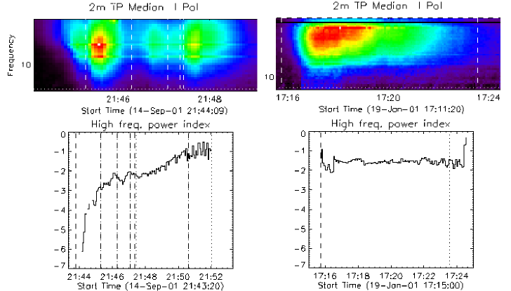
Figure 5: Two microwave bursts recorded by Owens Valley Solar Array in the range 1-18 GHz with 40 spectral channels and 4 sec temporal resolution. The first one (left bottom) displays evident spectral hardening with time, while the second one show remarkable constancy of the high-frequency spectral slope. Courtesy by D.E.Gary.

Nevertheless, as a rule the microwave emission from solar flares meets reasonable quantitative interpretation as synchrotron (gyrosynchrotron) radiation by moderately relativistic electrons (moving in non-uniform magnetic field of the coronal loop). An example of microwave burst produced by gyrosynchrotron emission is given in fig. 5, left.

Note, that the high-frequency spectral index $\delta$ (the radio flux is fitted by a power-law, $F\propto f^{\delta}$, at high frequencies, fig. 5, left bottom) decreases in value with time. Such spectral evolution typical for solar microwave bursts is well-understood in the context of the energy-dependent life time of electrons against the Coulomb collisions. Indeed, higher energy electrons have longer life time, which results in spectral hardening of trapped electron populationMelrose_Brown_1976 , and, respectively, hardening of the gyrosynchrotron radiation produced Melnikov_Magun_1998 .

However, if microwave emission is produced by diffusive synchrotron radiation as fast electrons interact with small-scale magnetic (and/or electric) fields, then the radio spectrum is specified by the spectrum of random fields rather then of fast electrons. Thus, no spectral evolution (related to electron distribution modification) is expected. Indeed, there is a minority of solar microwave bursts, which do not show any spectral evolution (e.g., no spectral hardening). An example of such a burst, demonstrating constancy in time of the high-frequency spectral index, is shown in fig. 5, right. Curiously, the spectral index is $\delta=-1.5-1.7$  in agreement with standard models turbulence and measurements of the turbulence spectra, e.g., in interplanetary Toptygin_83 and interstellar ISM space.

Although it has not been firmly proven so far, such microwave burst are possibly produced by diffusive synchrotron radiation mechanism. Since (to be dominant) this mechanism requires relatively dense plasma at the source site and soft spectra of accelerated electrons, the observational evidence can be found from analysis of simultaneous observations of soft and hard X-ray emissions from the same flares.

4 Discussion

The analysis presented demonstrates the potential importance of small-scale turbulence in the generation of electromagnetic emission from natural plasmas. This emission, being reliably detected and interpreted, provides the most direct measurements of small-scale turbulence in the remote sources. The diffusive synchrotron radiation is only one of the observable effects of the turbulence on the radio emission. Indeed, the presence of density inhomogeneities affects the properties of bremsstrahlung, because the Fourier transform of the square of the electric potential produced by background charges in a medium depends on spatial distribution of the charges through the double sum:

$$\mid\varphi_{q_{0},\vec{q}}\mid^{2}\propto\left<\sum_{A,B}e^{-i\vec{q}(\vec{R}_{A}-\vec{R}_{B})}\right>=\left[N+(2\pi)^{3}\frac{|\Delta N|^{2}_{\vec{q}}}{V}\right],$$ (49)

where $\vec{R}_{A}$ and $\vec{R}_{B}$ are the radius-vectors of particles $A$ and $B$ respectively, $|\Delta N|^{2}_{\vec{q}}$ is the spectrum of the inhomogeneities, $V$ is the volume of the system. In the uniform amorphous media the positions of various particles are uncorrelated and this double sum turns to be equal the total number of particles $N$. However, the macroscopic inhomogeneities make the positions correlated, so the double sum deviates from $N$. The second term in (49) gives rise to coherent bremsstrahlung, which dominates incoherent bremsstrahlung in a certain spectral range Pl_Topt_Fl_1990 .

Another important radiation process in the turbulent plasma is transition radiation arising as fast particles interact with small-scale density inhomogeneities of the background plasma (see Pl_Fl_2002 and references therein), whose potential importance for ionospheric conditions has been pointed out long ago Erm_Trakht_1981 (see also discussion in LaBelle ). This emission process, giving rise to enhanced low-frequency (at lower frequencies than accompanying synchrotron emission) continuum radio emission, has recently been reliably confirmed in a subclass of two-component solar radio bursts RTR ; RTR_letter . This finding is of particular importance for diagnostics of the number density, the level of small-scale turbulence, and the dynamics of low-energy fast particles in solar flares.

In addition, the turbulence can also affect the coherent emissions from unstable electron populations Fl_2004 , e.g., providing strong broadening (or splitting) of the spectral peaks generated by electron cyclotron maser (ECM) emission. The typical bandwidth of the broadened ECM peaks and its distributions are found to be quantitatively consistent with those observed for narrowband solar radio spikes Fl_2004 .

The National Radio Astronomy Observatory is a facility of the National Science Foundation operated under cooperative agreement by Associated Universities, Inc. This work was supported in part by the Russian Foundation for Basic Research, grants No. 03-02-17218, 04-02-39029. I am strongly grateful to T.S.Bastian for his numerous comments to the paper.

References

- (1) C.H. Jaroschek, H. Lesch, R.A. Treumann: ApJ 618, 822 (2005)
- (2) M. Honda, Y.S. Honda: ApJ 617, L37 (2004)
- (3) I.N. Toptygin: Cosmic rays in interplanetary magnetic fields (Dordrecht, D. Reidel 1985) 387 p
- (4) I.N. Toptygin, G.D. Fleishman: Astroph. & Space Sci. 132, 213 (1987)
- (5) A.B. Migdal: DAN SSSR 96, 49 (1954) (in Russian)
- (6) V.A. Razin: Izv. VUZov Radiofizika 3, 584 (1960)
- (7) V.L. Ginzburg, S.I. Syrovatsky: ARA&A 3, 297 (1965)
- (8) G.D. Fleishman: Astro-ph/0502245
- (9) Iu.A. Nikolaev, V.N. Tsytovich: Phys. Scripta 20, 665 (1979)
- (10) S. Jester, H.-J. Röser, K. Meisenheimer, R. Perley: A&A 431, 477 (2005)
- (11) G.M. Nita, D.E. Gary, J. Lee: ApJ 605, 528 (2004)
- (12) M.R. Kundu, S.M. White, N. Gopalswamy, J. Lim: ApJS 90, 599 (1994)
- (13) D.B. Melrose, J.C. Brown: MNRAS 176, 15 (1976)
- (14) V.F. Melnikov, A. Magun: Solar Phys. 178, 153 (1998)
- (15) S.I. Vainshten, A.M. Bykov, I.N. Toptygin: Turbulence, Current Sheets, and Shocks in Cosmic Plasma (The Fluid Mechanics of Astrophysics and Geophysics, Vol. 6) (Langhorne: Gordon and Breach Science Publ. 1993) 398 p
- (16) J.M. Cordes, M. Ryan, J.M. Weisberg, D.A. Frail, S.R. Spangler: Nature 354, 121 (1991)
- (17) K.Yu. Platonov, I.N. Toptygin, G.D. Fleishman: UFN 160(4), 59 (1990)
- (18) K.Yu. Platonov, G.D. Fleishman: UFN 172, 241 (2002) (transl.: Physics Uspekhi, 45, 235)
- (19) E.N. Yermakova, V.Yu. Trakhtengerts: Geomagn. and Aeron. (Engl. Edition), 21, 56 (1981)
- (20) J. LaBelle, R.A. Treumann: SSRv 101 295 (2002)
- (21) G.D. Fleishman, G.M. Nita, D.E. Gary: ApJ 620, 506 (2005)
- (22) G.M. Nita, D.E. Gary, G.D. Fleishman: ApJL 629, L65 (2005)
- (23) G.D. Fleishman: ApJ 601, 559 (2004)