A Search for sub-TeV Gamma-rays from the Vela Pulsar Region with CANGAROO-III

Abstract

We made stereoscopic observations of the Vela Pulsar region with two of the 10 m diameter CANGAROO-III imaging atmospheric Cherenkov telescopes in January and February, 2004, in a search for sub-TeV gamma-rays from the pulsar and surrounding regions. We describe the observations, provide a detailed account of the calibration methods, and introduce the improved and bias-free analysis techniques employed for CANGAROO-III data. No evidence of gamma-ray emission is found from either the pulsar position or the previously reported position offset by 0.13 degree, and the resulting upper limits are a factor of five less than the previously reported flux from observations with the CANGAROO-I 3.8 m telescope. Following the recent report by the H.E.S.S. group of TeV gamma-ray emission from the Pulsar Wind Nebula, which is $\sim$0.5 degree south of the pulsar position, we examined this region and found supporting evidence for emission extended over $\sim$0.6 degree.

1. Introduction

The Vela Pulsar is the brightest object in the sky at 100 MeV energies (Hartman et al., 1999), with emission extending beyond 10 GeV (Thompson et al., 2005). The emission at these energies is totally pulsed (Kanbach et al., 1994). The pulsar undergoes large glitches (e.g., Dodson et al., 2002), and has one of the highest values of $\dot{E}$/d² of all pulsars, making it a prime target for southern hemisphere searches for TeV gamma-rays (e.g., Nel et al., 1992). Early searches for TeV gamma-ray emission relied on the detection of a pulsed signal, and produced a number of suggestive but inconsistent results (see Edwards et al., 1994, for a review).

The first search sensitive to both pulsed and steady emission and made using the proven imaging atmospheric Cherenkov technique was undertaken with the CANGAROO-I 3.8 m telescope. A total of 119 hours of usable on-source data taken between 1993 and 1995 yielded a 5.8$\sigma$ excess, corresponding to a flux of (2.9$\pm$0.5$\pm$0.4) $\times$ 10^-12 cm^-2s^-1 above 2.5$\pm$1.0 TeV, offset from the Vela Pulsar by 0.13 degrees and with no significant modulation at the pulsar period (Yoshikoshi et al., 1997). A further 29 hours data from CANGAROO-I observations in 1997 showed a 4.1$\sigma$ excess at a position consistent with peak from the earlier observations (Yoshikoshi et al., 1997; Yoshikoshi, 1998). Observations by the Durham group in 1996 produced 3$\sigma$ upper limits above 300 GeV of $5\times 10^{-11}$ and $1.3\times 10^{-11}$ cm^-2s^-1 for steady and pulsed emission, respectively, at the pulsar position (Chadwick et al., 2000). No significant excess was found in a 2${}^{\circ}\times$2^∘ area centered at the pulsar position.

Based on independent Monte-Carlo simulations of the CANGAROO-I telescope (Dazeley & Patterson, 2001), Dazeley et al. (2001) searched for a TeV gamma-ray signal in the 29 hour 1997 dataset, but found no evidence of emission. Dazeley et al. (2001) noted that increasing the value of the length cut toward the value used in the earlier analysis did result in a somewhat increased excess, though not to a significant level, and acknowledged that the simulations had not included several known characteristics of the CANGAROO-I telescope hardware. An analysis of data from the Crab Nebula taken between December 1996 and January 1998 with two different sets of cuts also failed to yield a significant excess (Dazeley et al., 2001), although the resulting upper limit was higher than the established flux of the Crab Nebula. The TeV flux from the Crab Nebula from earlier CANGAROO-I (Tanimori et al., 1998) observations is consistent with the most recent measurements (Aharonian et al., 2004b).

The first preliminary results from observations with the H.E.S.S. stereoscopic imaging Cherenkov telescopes showed no evidence of emission from the Vela Pulsar nor from previous CANGAROO-I position (Khélifi et al., 2005). However, very recently the H.E.S.S. group reported the detection of broad TeV emission $\sim$0.5 degree south from the pulsar position extended over a region $\lesssim$ 0.6 degree (Khélifi et al., 2005b). The preliminary non-detection of emission from the pulsar was confirmed, yet the extended emission from the region of the Vela pulsar wind nebula was at the level of 0.5 crab (Khélifi et al., 2005b). Here we report the results from our observations of the Vela Pulsar region made in early of 2004 with the new CANGAROO-III stereoscopic imaging atmospheric system.

The previous CANGAROO-I analyses used slightly different cut values, especially in the image analyses, due in part to differences in source declination and sky brightness. Analysis using three or four image parameters requires selection of six to eight cut parameters (i.e., both upper- and lower-cut values for each parameter). While the cuts were guided by simulations, which endeavored to incorporate the characterstics of all telescope hardware and electronics (e.g., Dazeley & Patterson, 2001), any fine tuning introduces a number of degrees of freedom into the analysis, which can be difficult to account for a posteriori. The number of parameters can be reduced to one with the use of mathematical methods such as Likelihood (Enomoto et al., 2002) or the Fisher Discriminant (Fisher, 1936). In this report, we emphasize the application of such methods in order to remove any potentially biased operation from the analysis (see. e.g., Weekes, 2005). Previous CANGAROO-II analyses have been carried out using the Likelihood ratio, a Likelihood analysis with only one image cut (Enomoto et al., 2002). The Fisher Discriminant analysis introduced here now removes all cut uncertainties from the image analysis.

In §2 we describe the CANGAROO-III system, and in §3 we present the various calibration checks made to confirm its performance, introducing unbiased analysis methods based on Likelihood (Enomoto et al., 2002) and the Fisher Discriminant (Fisher, 1936). In §§4 and 5 the results of the CANGAROO-III observations of the Vela Pulsar and the surrounding field are presented, with conclusions given in §6.

2. The CANGAROO-III Stereoscopic System

The imaging atmospheric Cherenkov technique (IACT) was pioneered with the Whipple group’s detection of TeV gamma-rays from the Crab Nebula (Weekes et al., 1989). This technique enabled TeV gamma-rays to be distinguished from the huge background of cosmic rays with the use of the “Hillas moments” of the Cherenkov images (Hillas, 1985). Stereoscopic observations were successfully demonstrated by the HEGRA group to significantly improve the rejection of the cosmic ray background (Aharonian et al., 1999). More recently, the H.E.S.S. group has reported the detection of a number of faint gamma-ray sources with angular resolutions of only a few-arc minutes (Aharonian et al., 2005a).

The CANGAROO-III stereoscopic system consists of four imaging atmospheric imaging telescopes located near Woomera, South Australia (31^∘06’S, 136^∘47’E, 160 m a.s.l.). Each telescope has a 10 m diameter reflector consisting of 114 spherical mirror segments, each of 80 cm diameter and with an average radius of curvature of 16.4 m. The segments are made of Fiber Reinforced Plastic (FRP) (Kawachi et al., 2001) and are aligned on a parabolic frame with a focal length of 8 m. The total light collecting area is 57 m². The four telescopes are located on the corners of a diamond with spacings of approximately 100 m (Enomoto et al., 2002b). The first telescope, designated T1, is the CANGAROO-II telescope, and data from this telescope was not used in the analysis presented here as its smaller field of view (FOV) was less well suited for these stereoscopic observations. The second and third CANGAROO-III telescopes, T2 and T3, were used for the observations described here, with the fourth telescope (T4) becoming operational after these observations were completed. The camera systems for T2, T3, and T4 are identical and are described in detail in Kabuki et al. (2003). The pixel timing resolution is 1 ns at 20 photoelectron (p.e.) input. The noise level is 0.1 p.e. The relative gains of pixels are adjusted to within 10% at the hardware level by adjusting the high voltages applied to photomultipliers. The offline calibration are carried out using LED flasher data which were taken once per day. The gain uniformity of pixels is believed to be less than 5%.

The observations were made using the so-called “wobble mode” in which the pointing position of each telescope was alternated between $\pm$0.5 degree in declination from the center of the target every 20 minutes (Daum et al., 1997). Two telescopes, T2 and T3, were operational at this time, with T3 located 100 m to the south-south-east of T2. The data from each telescope were recorded with the trigger condition requiring that more than four pixels exceeded 7.6 p.e. The GPS time stamp was also recorded for each event. In the offline analysis, we combine these datasets by comparing the GPS timing. The distribution of timing differences is shown in Fig. 1.

Figure 1.— GPS time differences in units of $\mu$s for all events.

The broadness of the distribution was due to the time resolution of the GPS clocks. We required an off-line coincidence between the two telescopes’ trigger times within $\pm$100 $\mu$s. Events outside this time window were considered to be accidental coincidences. The trigger rates of the individual telescopes were at most 80 Hz and this was reduced to 8 Hz by requiring the above coincidence.

3. Calibration

In order to determine the sensitivity of the telescope, the efficiency of the light collecting system is the most important parameter to be precisely measured. Electromagnetic showers can be accurately simulated by computer code and cosmic ray showers can be observed in OFF-source observations and generated using Monte-Carlo codes such as GEANT. We measured the point spread function (PSF) and reflectivity of each mirror segment during their production and the quantum efficiency of each photomultiplier (PMT) pixel was also measured. Some deterioration in these values after the construction of the telescope is inevitable, and was monitored by regular PSF measurements of bright stars. Light collection efficiencies were monitored via optical systems such as photo-diodes and commercial CCD cameras observing stars both directly, and after reflection by the mirrors. These showed gradual degradation in the form of broadening spot sizes and decreasing reflectivities. However, these data only relate to the reflectors, and we need to know the total performance of the whole system including the cameras.

In order to measure these, we need “standard candles”; sources of Cherenkov photons or non-variable gamma-ray sources such as the Crab Nebula. Here, we introduce our calibration procedure using these methods.

3.1. Muon-ring Analysis

The ideal light source is one that produces the same Cherenkov radiation that the telescope is designed to detect. Sub-TeV cosmic rays produce hadronic showers in the upper atmosphere at a depth of around three inelastic interaction lengths, corresponding to an altitude of $\sim$10 km. Secondary hadrons are produced and interact further, with only gamma-rays, electrons and muons surviving to near ground level. Of these, relativistic muons radiate Cherenkov rings near the Earth’s surface, and these produce distinct complete or partial ring images on the camera.

The contribution of these rings to the trigger rate of our telescopes is critical, because small Cherenkov images resemble gamma-ray images. Local muon ring images can, however, be removed by requiring the coincidence of two or more telescopes separated by $\sim$100 m. Here, for calibration, we select images produced by muons at altitudes of 100–200 m. This can be done by selecting a somewhat larger “arc-length”. Arc-length is measured after fitting a circle to the images, and is the fitted radius multiplied by the recorded opening angle of the image. If larger images are required, we can simply restrict the selection to geometrically closer images such as those with altitudes $<$100–200 m. The inverse of the radius (curvature) should have a Gaussian distribution, so we therefore plot the curvature as a solid histogram in Fig. 2.

Figure 2.— Curvature distribution for the circular fitting results of all events for T3. The solid histogram is for all events and the dashed one for the selected events (with the vertical scale multiplied by 5).

A peak can be seen around 1/1.3 [1/degree] which corresponds to the inverse of the Cherenkov angle initiated by relativistic muons at normal temperature and pressure. The distribution for T2 (which was constructed before T3), however, was not as good, indicating some degradation in its performance, as shown by the solid histogram in Fig. 3.

Figure 3.— Curvature distribution for the circular fitting results on all events for T2. The solid histogram is for all events and the dashed one for the selected events (with the vertical scale multiplied by 5).

These data were taken in 2003 December. We need to know our light collection efficiency in each observing period, i.e., we need to improve the S/N ratio to select a pure muon-ring sample only. The following are the cut criteria used to achieve this.

• Hit threshold more than 1 photo-electron (p.e.).

• TDC range within $\pm$30 ns from the mean arrival time of the event.

• At least 15 triggered (or “hit”) PMTs, with a clustering requirement that there be at most two non-triggered PMTs between nearest-neighbor hit PMTs.

• A circle, or ring segment, can be fitted to the image.

• The circle has an “arc-length” of more than 2 degrees.

• A $\chi^{2}$ per hit-pixel, normalized to the pixel size, of less than 1.5.

The curvature distributions of the samples meeting these criteria are shown as dashed histograms in Figs. 2 and 3. Muon ring events are selected with a good S/N ratio. Geometrically, the arc-length cut restricts selection to events occurring at $<$100–200 m. The statistics of the accepted events are sufficient for calibration to be undertaken with only several hours data.

There is some dependence of light yield on the atmospheric temperature; however, this is monitored and recorded every second. The night-time temperature near Woomera ranges from near 0 C in winter to over 30 C in summer. The systematic error, which includes the reflectivity of the present mirror, the PSF, and the quantum efficiency of the PMTs, is thought to be at the 5% level of the total light collection efficiency. The light collection efficiencies can be derived from the “size/arc-length” distribution and the PSFs by the $\chi^{2}$ of the ring fits. The observation periods for the Crab Nebula and Vela Pulsar data considered here were between the end of 2003 and the beginning of 2004.

The calibrated light collection efficiencies for T2 and T3 were both 70%, with 5% systematic errors. These values are the ratios of the efficiencies derived during the observation period and those measured at the production time, i.e., the deterioration factors. The PSFs were approximated by Gaussian distributions with standard deviations of 0.14, and 0.12 degrees, respectively, which are somewhat larger than the results obtained via bright star measurements at the initial installation time. (The corresponding values for T4, which was just coming on-line, were 85% and 0.09 degrees, respectively.) The $\chi^{2}$ distributions for the experiments (the solid histogram) and the tuned Monte-Carlo simulations (the hatched area) are shown in Fig. 4 for T2 (upper panel) and T3 (lower panel).

Figure 4.— Distributions of $\chi^{2}$ for the experimental data and the tuned Monte-Carlo. The solid histograms are the experimental data and the hatched the Monte-Carlo. The upper panel is for T2 and the lower T3.

The PSF of T2 is worse than that of T3. The size/arc-length distributions for the experiments (the solid histogram) and the tuned Monte-Carlo (the hatched area) are shown in Fig. 5 for T2 (upper panel) and T3 (lower panel).

Figure 5.— Distributions of size/arc-length for the experimental data and the tuned Monte-Carlo. The solid histograms are the experiment and the hatched the Monte-Carlo. The upper panel is for T2 and the lower T3.

The PSFs obtained for the three telescopes are somewhat larger than those of H.E.S.S., corresponding to a relatively lower cosmic-ray rejection efficiency. The resulting S/N ratio for gamma-rays is discussed in the next section; however, it is sufficient to detect gamma-ray sources with flux levels flux of $\sim$0.1 Crab in several tens of hours.

The measured efficiencies do not depend strongly on climate or atmospheric conditions, as they are local (near-surface) phenomena. Thus uncertainty due to Mie scattering, for instance, still remains. This is thought to be significant at the 10% level; however, the average effect can be gauged in the Crab Nebula data described in the following section. In fact, data taken during cloudy nights showed a better S/N ratio in the curvature distribution. As the muon rings are a local phenomenon, there is naturally no dependence on the elevation angle of the observation, whereas the cosmic ray rate varies strongly with elevation. Using these characteristics, we were able to measure the degradation as a function of time for the three telescopes (T2, T3, and T4), with the light collection efficiency being found to decrease by 5% per year. Hereafter in the analyses of the individual sources, we used muon-ring data from the corresponding periods to tune our Monte-Carlo code.

3.2. Crab Analysis

The description on the Crab data used in the following section can be found in Appendix A. At first, the Hillas moments were calculated for each telescope’s image. The intersection of the major axes of the two images is the incident direction of the gamma-ray in the stereoscopic observation. The $\theta^{2}$ distribution of the Monte-Carlo data for this observation condition calculated from the intersection points is plotted in Fig. 6 (the dashed line).

Figure 6.— $\theta^{2}$ distributions from Monte-Carlo simulations. The dashed line is obtained without the fitting procedure described in the text and the solid line is that with it.

The angular resolution is, as expected, several times worse than that of H.E.S.S. (Aharonian et al., 2004), due to the larger PSFs described above. The Crab Nebula observations were carried out at relatively low elevation angles and the opening angle between the T2 and T3 images are typically small, resulting in many parallel images. This results in an increased uncertainty in the intersection point of the two images. To avoid this, we reanalyzed the data with a constraint on the distances between images’ center of gravity and the intersection point. (H.E.S.S. observations are made at elevation angles typically 10 degrees higher and with smaller mirror PSF, resulting a good S/N ratio without this constraint. If the PSFs of mirrors were as small as specified in the original design, we could also avoid this procedure.) The $\chi^{2}$ was defined as

$$\sum_{T=2,3}\left[W_{T}^{2}+\frac{(D_{T}-\langle Distance\rangle)^{2}}{\sigma_{Distance}^{2}}\right],$$

where $W_{T}$ is the width seen from the intersection point, and $D_{T}$ is the distance between the image center of gravity and the intersection for each telescope (Fig. 7), $\langle Distance\rangle$ is the mean distance obtained by Monte-Carlo simulations for gamma-rays, and $\sigma_{Distance}$ is its standard deviation.

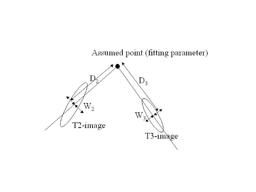
Figure 7.— Definitions of parameter $W_{T}$ and $D_{T}$ which are used in the fitting procedure described in the text.

The improved $\theta^{2}$ distribution is shown as the solid line in Fig. 6. The number of events with $\theta^{2}<$ 0.05 degree² increases by a factor of 1.8. Note that the angular resolution was estimated to be 0.23 degree and 0.23² is roughly 0.05 degree².

We first used the conventional (“square cuts”) method as follows; we accepted events with width $<$ 0.2 (for T2) and 0.15 (for T3), and length $<$ 0.3 (for T2) and 0.25 (for T3), respectively, where all values are in units of degrees. The cut values differ for T2 and T3 due to the PSF differences. As the $\theta$ resolution is 0.23 degree, we took six background points on the 0.5-degree-radius circle from the pointing direction. The resulting $\theta^{2}$ distributions for the ON-source points (the points with error bars) and the OFF-source points (the solid histogram) are shown in Fig. 8.

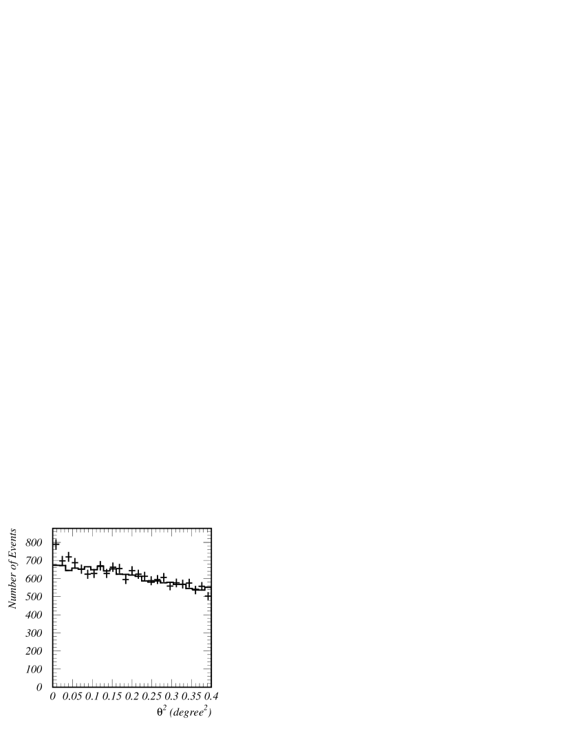
Figure 8.— $\theta^{2}$ distribution for the standard analysis of Crab Nebula data. The points with error bars are from the ON-source region and the solid histogram is the background region.

The background normalization factor is 1/6, equal to the inverse of the number of background points in these wobble mode observations. The number of excess events with $\theta^{2}<0.05$ degree² is (2207$-$1990=) 216, where the numbers in parentheses are the on-source and estimated background counts, respectively. This corresponds to a Li & Ma (1983) significance of 4.4$\sigma$. The number of events predicted by our Monte-Carlo simulation, using the Aharonian et al. (2000) flux, an $E^{-2.5}$ gamma-ray energy spectrum, and minimum and maximum gamma-ray energies of 500 GeV and 20 TeV, was 195 events. (For comparison, we also undertook “mono”, i.e., single telescope, analyses using the regular CANGAROO-II procedures. Excesses for both telescopes were found using both by square cut and Likelihood cut analyses. The statistical significances of these excesses were at the 3$\sigma$ level, confirming the power of the stereo technique.)

Using the events with $\theta^{2}<0.05$ degree², we can derive the Hillas moment distributions after background subtractions. This provides a check of how well the Monte-Carlo simulations agree with the real gamma-ray data. These are shown in Fig. 9.

Figure 9.— Hillas moment distributions: upper-left (T2 widths), upper-right (T2 lengths), lower-left (T3 widths), and lower-right (T3 lengths). The points with error bars were obtained after the subtraction of background events. The solid histograms are the Monte-Carlo predictions where the total number of entries were normalized to those of the observations.

Our Monte-Carlo simulations are consistent with the data within statistical uncertainty. Note that the width distribution is sensitive to the PSF of the mirror system and that that of T3 is better than T2.

After this standard analysis, we investigated two bias-free analyses. The first is the Likelihood method introduced by Enomoto et al. (2002). In the standard “square cuts”, there are four parameters on which cuts can be made, and in the absence of a strong gamma-ray source or detailed simulations accurately incorporating the characteristics of the telescope hardware, some freedom in choosing the exact cuts is available. (see, e.g., the discussion in Dazeley et al., 2001). In the Likelihood method, we proceed by making probability density functions (PDFs) from the histograms of width and length, for the two telescopes, and some other parameters such as the opening angle and the distance between two images’ center of gravity (image separation) (Fig. 10).

Figure 10.— Distributions of opening angle and separation angle of two images. These were obtained also via the subtraction described above for the Crab data.

In order to treat the energy dependence of these parameters, we used two-dimensional histograms: the PDFs are therefore 2-D functions. For the gamma-ray sample, we used the data from Monte-Carlo simulations, and for the cosmic ray background sample, we used real observation data, since the “contamination” by gamma-rays is much less than 1%. Thus for each event, we can derive a probability ($L$) for the event being initiated by a gamma-ray or a cosmic ray, where normalization ambiguities still remain. The Likelihood ratio $LR$ is defined as

$$LR=\frac{L(gamma-ray)}{L(background)+L(gamma-ray)}.$$

The distributions for the Crab Nebula data are shown in Fig. 11.

Figure 11.— Likelihood Ratio ($LR$) distributions. The points with error bars are from Crab Nebula gamma-rays, the solid histogram from the gamma-ray Monte-Carlo, and the dashed histogram from all events. The latter two distributions are normalized to the total number of the observed excess.

The observational data are in reasonable agreement with the Monte-Carlo predictions. Observationally, the optimal cut was found to be $LR>$0.9. The number of excess events is (390$-$289=) 101 (a Li and Ma significance of 5.2 $\sigma$) where the Monte-Carlo expectation is 121 events. The determination of the cut position is, however, still somewhat subjective.

A simple figure of merit — the number of the accepted events in the Monte-Carlo simulation divided by the square-root of those in the observation — is plotted as a function of $LR$ in Fig. 12.

Figure 12.— Statistical significance of the Crab excess versus $LR$ cut position (the solid line). The dashed curve is the figure of merit calculated as described in the text. The normalization is arbitrary.

The Monte-Carlo prediction is a smoothly increasing function of the cut position (the dashed line). On the other hand, the statistical significance of the observed excess is shown by the solid line. The two show good agreement over a wide range; however, some discrepancy is apparent in the extremely tight cut positions. For example, a $LR$ cut at 0.5 gives an excess (Fig. 13), of (1049$-$895=) 154 events (4.6$\sigma$) where the expectation is 182 events.

Figure 13.— $\theta^{2}$ distribution for Crab Nebula data obtained using the $LR>$ 0.5 cut.

Further fine-tuning of the Monte-Carlo code is necessary in the future and such tight cuts will for now be avoided. The optimal cut position of 0.9 is located on the edge of this tight cut region.

We now investigate an alternative approach for the comparison of observational and Monte-Carlo data: the Fisher Discriminant (Fisher, 1936). When we use multi-parameters:

$$\vec{P}=(Vector~{}of~{}Hillas~{}moments~{}for~{}two~{}telescopes)$$

and assume that a linear combination of

$$F=\vec{\alpha}\cdot\vec{P},$$

provides the best separation between signal and background, then the set of linear coefficients ($\vec{\alpha}$) should be uniquely determined as

$$\vec{\alpha}=\frac{\vec{\mu}_{sig}-\vec{\mu}_{BG}}{E_{sig}+E_{BG}},$$

where $\vec{\mu}$ is a vector of the mean value of $\vec{P}$ for each sample, i.e., $=\langle\vec{P}\rangle$, and $E$ is their error matrix, i.e., $=\langle\vec{P}\vec{P}^{T}\rangle-\langle\vec{P}\rangle\langle\vec{P}^{T}\rangle$. The values of $\vec{\mu}_{sig}$, $\vec{\mu}_{BG}$, $E_{sig}$, and $E_{BG}$ can be calculated from the Monte-Carlo gamma-ray events for signal and observational data for background. Our purpose is to separate “sharp images” from “smeared ones”. This method is regularly used in high-energy physics experiments, such as the $B$-factory’s “Super Fox-Wolfram moment” (Abe et al., 2001), in order to separate spherical events from jet-like events. Here, the assumption strongly depends on which linear combination is best. We must, therefore, select parameters which are similar to each other. Width and length are both second order cumulative moments of shower images and thus a linear combination is a reasonable assumption. We used four image parameters: T2-width, T3-width, T2-length, and T3-length. Here, the energy dependence of width and length for each telescope were corrected using the energy estimated from the summation of ADC values of hit pixels for that telescope using the Monte-Carlo expectations. This correction function was a second-order polynomial and we carry out an offset correction using it, i.e.,

$$\vec{P}=\vec{P}_{raw}-\vec{a}_{0}-\vec{a}_{1}log(\sum ADC)-\vec{a}_{2}log(\sum ADC)^{2},$$

where $\vec{a_{i}}$s were determined from the two-dimensional plots of raw “Hillas moments” versus $log(\sum ADC)$ using the Monte-Carlo gamma-ray simulations and $\vec{P}_{raw}$ is a vector made of the raw values of “Hillas moments”, respectively. The corrected width and length are distributed around zero and the $\langle\vec{P}_{sig}\rangle$ is automatically located exactly at zero,

$$\langle\vec{P}_{sig}\rangle=0$$

resulting in the Monte-Carlo expectation of $F$ location being zero:

$$\langle F_{sig}\rangle=0.$$

This removes cut-selection bias: a cut at zero ensures 50% acceptance (for gamma-rays) automatically, a typical value adopted in IACT analyses. From the $\theta^{2}$ Crab Nebula excess we obtain the following distribution of Fisher Discriminant, $F$, as shown in Fig. 14.

Figure 14.— Distributions of the Fisher Discriminant, $F$. The points with error bars are obtained from the observation, the solid histogram from the gamma-ray Monte-Carlo, and the dashed from all events representing background behavior.

The behavior of the distributions for gamma-ray signals, background events, and Monte Carlo expectations agree reasonably well and are similar or a little bit better than the result obtained for the Likelihood method. This figure should be compared with Fig. 2 in the recently published H.E.S.S. paper for the distribution of their mean reduced scaled width (Aharonian et al., 2005b). The H.E.S.S. discrimination is better; however, improved results can be expected for CANGAROO-III if the quality of mirrors were improved to the levels of H.E.S.S. or MAGIC.

We consider the figure of merit for this method in Fig. 15.

Figure 15.— Statistical significance of the Crab Nebula excess versus $F$ cut position (the solid line). The dashed curve is the figure of merit calculated as described in the text. The normalization is arbitrary.

This time, the agreement is very good in all regions. Although the cut at $F>-$0.16 showed the best statistical significance, 5.8$\sigma$, with an excess of (1177$-$974=) 203 events, where the Monte-Carlo expectation is 162 events. A conservative choice of cut point is zero which, as noted above, is exactly the mean expected position for a gamma-ray acceptance of 50%. In the following we use the Fisher Discriminant analysis as the default, with a cut position at zero, thus removing all subjective or potentially biased elements from the analysis. The excess is (744$-$604=) 140 events, where the expectation is 110 events. The final $\theta^{2}$ distribution is shown in Fig. 16.

Figure 16.— The final $\theta^{2}$ plot for the Crab Nebula, using the Fisher Discriminant analysis with the cut at zero.

In this analysis, we estimated the gamma-ray energy using the average of the T2 and T3 summations of ADC values, which probably provides the optimal energy resolution for this analysis. The usage of the intersection constraint, due to finite point spread function of the individual mirror segments, does not allow a core-distance correction of energy. The overall energy resolution was considered to be 30% from the simulation study. We show the differential flux for the Crab Nebula in Fig. 17.

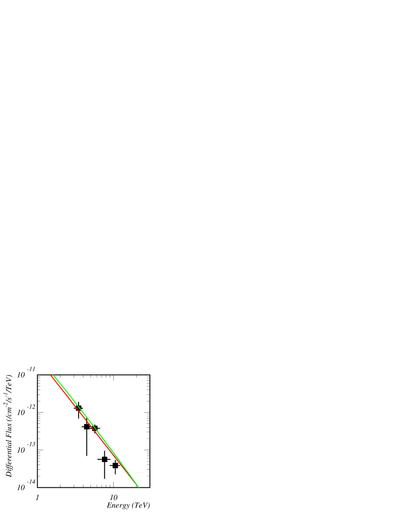
Figure 17.— Differential gamma-ray flux from the Crab Nebula as a function of energy. The red line is the HEGRA result (Aharonian et al., 2000) and the green is the Whipple result (Hillas et al., 1998).

The points with error bars are our data where the errors are statistical. The systematic error is considered to be 15% at this stage. HEGRA (Aharonian et al., 2000) and Whipple (Hillas et al., 1998) results are also shown. The results agree within the statistical and systematic errors. The deviation in the CANGAROO flux at higher energies may be due to saturation effects, which are not yet fully implemented in our Monte-Carlo code; however, this in not an important consideration for Vela observations, which are the main focus of this paper. We leave further consideration of this for the future, noting that while the analysis template defined here for CANGAROO-III is, at present, most suitable, it may be able to be further optimized with refined Monte-Carlo simulations.

We show the 2D profile of gamma-ray images in Fig. 18.

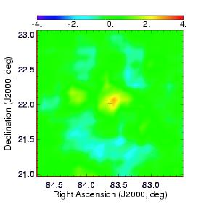
Figure 18.— Excess number plot in the equatorial frame. The unit is events per $0.1\times 0.1$ degree² in the FOV coordinates. The cross indicates the center of the Crab Nebula. The resolution is considered to be 0.23 degrees in declination in this frame.

The angular resolution is estimated to be 0.23 degrees (1$\sigma$). Here, only high energy events ($E>$10.6 TeV) are plotted in order to improve the S/N ratio and to remove uncertainties in the background subtraction. The background level at each position was estimated using the events with values of $F$ below $\langle F_{BG}\rangle$ which are considered to be mostly background protons. Here, however, we need to note that the subtraction template for the background was made using events with low $F$ sample. The Fisher Discriminant uses a linear combination of the energy-corrected width and length for T2 and T3, respectively. The subtraction sample for morphological studies may tend to be overwhelmed by the larger sized events which have poorer angular resolutions. The important thing is that the background sample tends to be flatter than the gamma-ray events. Therefore, we only show a very restricted area in this figure. An improved analysis, required for diffuse gamma-ray detection, which will be introduced later.

As a result of the considerations above, the analysis template is:

• the Fisher Discriminant is adopted.

• the cut position on $F$ is exactly at zero.

• others parameters, such as elevation cut and shower-rate cut, are determined as appropriate for the source under investigation (depending on its declination and galactic coordinates).

4. Observations of the Vela Pulsar

The Vela Pulsar was observed between 2004 January 17 and February 25. In total, the preselected data correspond to an analyzable period of 1311 min. after the elevation and cloud cuts, where the minimum elevation angle was set at 60 degrees and the shower rate at 9 Hz. The mean elevation angle was 70.9 degrees, corresponding to an energy threshold of 600 GeV. The observations were carried out using the same wobble mode as for the Crab Nebula observations. In this period, T2 and T3 were in operation and we analyzed the stereo data from these two telescopes. As the Vela Pulsar is at a declination of $-$45^∘, the relative orientation of the two telescopes does not present any problems.

We used the optimized analysis procedure described in the previous section and so there are no a posteriori trials to consider in the interpretation of results — it is a “blind analysis”. The resulting $\theta^{2}$ distribution is shown in Fig. 19.

Figure 19.— The $\theta^{2}$ distribution for Vela Pulsar observations resulting from application of the analysis template described in §3.3.

After the background subtraction, we obtained an excess of (677$-$722=) $-$45$\pm$29 events. Monte Carlo simulations, with minimum and maximum gamma-ray energies of 100 GeV and 20 TeV, respectively, and an energy spectrum proportional to $E^{-2.5}$, predict 394 events would be detected for a 100% Crab level gamma-ray source. The CANGAROO-I flux was 60% of the Crab Nebula flux. The $F$ distribution, obtained using subtraction, is shown in Fig. 20.

Figure 20.— $F$ distributions. The points with error bars are obtained from the observations, the solid curve from the gamma-ray Monte-Carlo simulations, and the dashed histogram from all observed events to represent the cosmic ray background behavior. The Monte-Carlo histogram is normalized to a 100% Crab Nebula flux level.

There is no excess of gamma-ray–like events around the predicted region, offset by 0.13 degrees from the Vela Pulsar. Thus observations with significantly improved instrumentation and a robust analysis procedure do not support the previous claim for TeV gamma-ray emission from this region.

The 2$\sigma$ upper limits are shown in Fig. 21, together with the results of other observations.

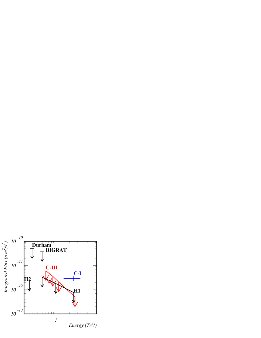
Figure 21.— 2$\sigma$ upper limits for the gamma-ray flux. C-I represents the CANGAROO-I result (Yoshikoshi et al., 1997) and C-III indicates the CANGAROO-III result reported here. Also shown are Durham (Chadwick et al., 2000), BIGRAT (Dazeley, 1999) and H.E.S.S. preliminary results (Khélifi et al., 2005) (Khélifi et al., 2005b).

The upper limits in the figure are a factor of 5 below the CANGAROO-I result. This analysis has used the point offset by 0.13 degrees to the south-east of the Vela Pulsar, i.e., offset is ($\Delta$RA,$\Delta$dec)=(0.14^∘,$-$0.1^∘) from the pulsar position. This position which was the maximum of the excess detected with the CANGAROO-I telescope: an analysis at the position of the Vela Pulsar position yields similar upper limits. These are summarized in Table 1.

Table 1 2-$\sigma$ upper limits to the integrated fluxes.

	$F$($>E$) at	$F$($>E$) at
Energy, $E$	offset position	pulsar position
(GeV)	(cm-2s-1)	(cm-2s-1)
600	$<5.8\times 10^{-12}$	$<5.8\times 10^{-12}$
710	$<4.5\times 10^{-12}$	$<4.5\times 10^{-12}$
860	$<3.4\times 10^{-12}$	$<3.4\times 10^{-12}$
1200	$<2.0\times 10^{-12}$	$<2.4\times 10^{-12}$
2700	$<4.7\times 10^{-13}$	$<4.7\times 10^{-13}$

5. Vela Pulsar Wind Nebula

Recently, extended TeV gamma-ray emission coincident with the Vela Pulsar Wind Nebula (PWN) was reported by the H.E.S.S. group (Khélifi et al., 2005b). Their preliminary report claimed that the center of the emission is (RA, dec) = (8^h35^m, $-$45^∘36^′) and that the flux within a 0.6 degree radius from this position is 50% of the Crab Nebula at 1 TeV. They also noted that no gamma-rays were detected from the Vela Pulsar, and placed a tight upper limit on the pulsar flux at 0.26 TeV (Khélifi et al., 2005, 2005b).

Thus far, we have focused on a point source analysis based on the wobble mode observations. The peak PWN source position coincides with the one of two wobble pointing direction in the coordinate of the field of view of the camera. We, therefore, can not carry out background estimation using the usual wobble method. In this section we undertake an optimized analysis for an extended source. Another difficulty is that we don’t have sufficient statistics for OFF source regions, and so the background subtractions should be carried out using the ON source data runs. Gamma-ray–like events can be extracted by fitting position-by-position $F$ distributions under the assumption that gamma-rays obey the Monte-Carlo predictions, the proton background follows the average $F$ distribution of all directions, and the total distribution is a linear combination of those two. The separation between those two distributions is likely to be worse at lower energies due to the smaller image sizes. These distributions are plotted in Figs 22 for various energy ranges.

Figure 22.— $F$ distributions in various energy regions. The blank histograms are for Monte Carlo simulations of gamma-rays and the hatched histograms for background regions of real data. From the top panel to the bottom, the central gamma-ray energies are 540, 780, 1200, 2700, 3300, and 8800 GeV, respectively. The histogram entries are normalized to one event in the shown regions.

From the upper to lower panels, the central energies of the energy bins are 540, 780, 1200, 2700, 3300, and 8800 GeV, respectively. The blank histograms are gamma-rays and the hatched, protons. As shown in figure, the separation begins at 780 GeV and becomes significant at 1200 GeV. Therefore, we first analyzed events with energy greater than 1200 GeV.

Then we checked the directional dependence of the $F$ distributions. The field of view was segmented into 0.2$\times$0.2 degree² regions and each $F$ distribution was compared with the average. The reduced $\chi^{2}$ distribution is shown by the histogram in Fig. 23.

Figure 23.— Reduced $\chi^{2}$ distribution for various arrival directions (the histogram). The pixel size for each direction is 0.2 $\times$ 0.2 degree². The curve is the expected distribution for the number of degrees of freedom, 23.

The curve shown is the predicted distribution for the 23 degrees of freedom. There is good agreement, i.e., there is no significant directional dependence.

This method was then checked with Crab Nebula data. The $F$ distributions at various $\theta^{2}$ slices were taken at energies greater than 5.7 TeV. The background $F$ distribution was obtained in the higher $\theta^{2}$ region, 0.1–0.3 degree². The only fitting parameter is the percentage of gamma-ray–like events relative to the total events. The result is shown in Fig. 24.

Figure 24.— The $\theta^{2}$ plot obtained by the fitting method described in the text for Crab Nebula data. The vertical scale is the percentage of gamma-ray–like events relative to all events.

The statistical significance of the peak is 4.0$\sigma$, while the ordinary wobble analysis gave a 3.6$\sigma$ excess.

Having demonstrated the validity of this method, we carried out an analysis of the Vela PWN region. The H.E.S.S. group detected a gamma-ray excess extended over a 0.6 degree radius from the center of the emission [(RA, dec) = (8^h35^m, $-$45^∘36^′)]. In our case, the angular resolution (0.23 degree) is significantly worse than that of H.E.S.S. We, therefore, chose the background region to be more than 0.8 degree from the center. The result of fitting is shown in Fig. 25.

Figure 25.— The wide range $\theta^{2}$ plot for the Vela PWN region, where $\theta$ was calculated from (RA, dec) = (8^h35^m, $-$45^∘36’), i.e., the peak of the emission detected by H.E.S.S. The gamma-ray–like events were extracted by the fitting procedure described in the text.

An excess was observed at $\theta^{2}<0.6$ degree² around the center of Vela PWN region. The excess radius is marginally consistent with H.E.S.S. considering our angular resolution. The total number of gamma-ray–like events is 561$\pm$114.

The differential flux was obtained and is shown in Fig. 26.

Figure 26.— Gamma-ray flux in the Vela PWN region.

Although the statistics are poor, the spectrum looks hard, consistent with the preliminary H.E.S.S. results, and the fluxes are in general agreement. This excess is below the 5$\sigma$ level generally required for a firm detection (Weekes, 2005) and is spatially extended over a significant portion of our field of view, and thus a high resolution (0.1 degree) morphology map is not justified. We are, however, able to offer supporting evidence of the H.E.S.S. result and, in this light, are planning to observe the PWN region in more detail next year.

6. Conclusion

We have observed the Vela Pulsar region from 2004 January 17 to February 25 with the CANGAROO-III stereoscopic imaging Cherenkov telescopes. At that time, two telescopes (T2 and T3) were in operation and events coincident to the two telescopes were analyzed. Calibration was performed using muon rings and the performance of the telescopes confirmed with observations of the Crab Nebula. The estimated energy threshold for this analysis was 600 GeV. The use of the Fisher Discriminant has been introduced and a template for CANGAROO-III analysis presented. No significant excess of events was found from the Vela Pulsar direction or from the peak of the emission detected with the CANGAROO-I telescope. The upper limits obtained are a factor of five less than the CANGAROO-I fluxes (assuming an $E^{-2.5}$ spectrum). In addition, we have confirmed, at the 4$\sigma$ level the gamma-ray emission recently reported from the Vela Pulsar Wind Nebula. The TeV emission from the PWN peaks $\sim$0.5 degree south of the pulsar position and has a $\sim$0.6 degree extension, consistent with the H.E.S.S. report. A detailed morphological study of this source will require more observations.

Appendix A Crab Observation

Observations of the Crab Nebula were carried out over the period 2003 December 18 to 28. The observations were made using the so-called “wobble mode” in which the pointing position of each telescope was alternated between $\pm$0.5 degree in declination from the center of the Crab Nebula every 20 minutes (Daum et al., 1997). Two telescopes, T2 and T3, were operational at this time. T3 is located 100 m to the south-south-east of T2, which is not ideal for observations of northern sources; however sufficient data was recorded for a useful analysis to be made. The trigger rates of the individual telescopes were at most 80 Hz and this was reduced to 8 Hz by requiring the above coincidence. The total observation time was 1122 min. Next we required both telescopes to have clusters of PMTs with five adjacent hits above a 5 p.e. hit threshold, which reduced the event rate to 6 Hz. Looking at the time dependence of this event rate, we can remove data taken in cloudy conditions. This procedure is exactly the same as the “cloud cut” used in CANGAROO-II analysis (Enomoto et al., 2002). Only data taken at elevation angles greater than 30 degrees were used, resulting in a total of 890 minutes data, with a mean elevation angle of 35 degrees.

References

- Abe et al. (2001) Abe, K., et al., 2001, Phys. Rev. Lett., 87, 101801
- Aharonian et al. (1999) Aharonian, F. A., et al., 1999, A&A, 349, 11
- Aharonian et al. (2000) Aharonian, F. A., et al., 2000, ApJ, 539, 317
- Aharonian et al. (2004) Aharonian, F. A., et al., 2004, A&A, 425, L13
- Aharonian et al. (2004b) Aharonian, F., et al., 2004b, ApJ, 614, 897
- Aharonian et al. (2005a) Aharonian, F. A., et al., 2005a, Science, 307, 1938
- Aharonian et al. (2005b) Aharonian, F. A., et al., 2005b, A&A, 439, 1013
- Chadwick et al. (2000) Chadwick, P.M., et al., 2000, ApJ, 537, 414
- Daum et al. (1997) Daum, A., et al. 1997, Astropart. Phys., 8, 1
- Dazeley (1999) Dazeley, S. A., 1999, A search for very high energy gamma-ray emission from four Galactic pulsars, PhD thesis, University of Adelaide
- Dazeley & Patterson (2001) Dazeley, S. A., and Patterson, J. R., 2001, Astropart. Phys., 15, 305
- Dazeley et al. (2001) Dazeley, S. A., Patterson, J. R., Rowell, G. P., & Edwards, P. G., 2001, Astropart. Phys., 15, 313
- Dodson et al. (2002) Dodson, R. G., McCulloch, P. M., & Lewis, D. R. 2002, ApJ, 564, L85
- Edwards et al. (1994) Edwards, P. G., Thornton, G. J., Patterson, J. R., Roberts, M. D., & Rowell, G. P. 1994, A&A, 291, 468
- Enomoto et al. (2002) Enomoto, R., et al. 2002b, Nature, 416, 823
- Enomoto et al. (2002b) Enomoto, R., et al. 2002a, Astropart. Phys., 16, 235
- Fisher (1936) Fisher, R. A., 1936, Annals of Eugenics, 7, 179
- Hartman et al. (1999) Hartman, R. C., et al. 1999, ApJS, 123, 79
- Hillas (1985) Hillas, A. M., Proc. 19th Int. Cosmic Ray Conf. (La Jolla) 3, 445
- Hillas et al. (1998) Hillas, A. M., et al., 1998, ApJ, 503, 744
- Kabuki et al. (2003) Kabuki, S., et al., 2003, Nucl. Instrum. Meth., A500, 318
- Kanbach et al. (1994) Kanbach, G., et al., 1994, A&A, 289, 855
- Kawachi et al. (2001) Kawachi, A., et al., 2001, Astropart. Phys., 14, 261
- Khélifi et al. (2005) Khélifi, B., et al. 2005, AIP Conf. Proc. 745, International Symposium on High Energy Gamma-Ray Astronomy, ed. F. A. Aharonian, H. J. Völk, & D. Horns (New York: AIP), 335
- Khélifi et al. (2005b) Khélifi, B., et al., 2005b, Proc. 29th Int. Cosmic Ray Conf., (Pune), OG2.2, 101
- Li & Ma (1983) Li, T. and Ma, Y., 1983, ApJ, 272, 317
- Nel et al. (1992) Nel, H. I., Raubenheimer, B. C., de Jager, O. C., Brink, C., Meintjes, P. J., North, A. R., & van Urk, G. 1992, ApJ, 398, 602
- Tanimori et al. (1998) Tanimori, T., et al., 1998, ApJ., 492, L33
- Thompson et al. (2005) Thompson, D. J., Bertsch, D. L., & O’Neal, R. H. 2005, ApJS, 157, 324
- Yoshikoshi et al. (1997) Yoshikoshi, T., et al., 1997, ApJ, 487, L65
- Yoshikoshi (1998) Yoshikoshi, T., 1998, “Neutron Stars and Pulsars — thirty years after the discovery”, ed. Shibazaki, N., et al., (Tokyo: University Academy Press) 479.
- Weekes et al. (1989) Weekes, T. C., et al., 1989, ApJ, 342, 379
- Weekes (2005) Weekes, T., 2005, astro-ph/0508253